Quantization Audio Watermarking with Optimal Scaling on Wavelet Coefficients S.-T. Chen, H.-N. Huang, and S.-Y. Tu
Abstract—In recent years, discrete wavelet transform (DWT) provides an useful platform for digital information hiding and copyright protection. Many DWT-based algorithms for this aim are proposed. The performance of these algorithms is in term of signal-to-noise ratio (SNR) and bit-error-rate (BER) which are used to measure the quality and the robustness of an embedded audio. However, there is a tradeoff relationship between the embedded-audio quality and robustness. The tradeoff relationship is a signal processing problem in the wavelet domain. To solve this problem, this study presents an optimization-based scaling scheme using optimal multi-coefficients quantization in the wavelet domain. Firstly, the multi-coefficients quantization technique is rewritten as an equation with arbitrary scaling on DWT coefficients and set SNR to be a performance index. Then, a functional connecting the equation and the performance index is derived. Secondly, Lagrange Principle is used to obtain the optimal solution. Thirdly, the scaling factors of the DWT coefficients are also optimized. Moreover, the invariant feature of these optimized scaling factors is used to resist the amplitude scaling. Experimental results show that the embedded audio has high SNR and strong robustness against many attacks.
Index Terms—Discrete wavelet transform, signal-to-noise ratio, bit-error-rate, optimal scaling, invariant feature.
I. INTRODUCTION Generally, an audio watermarking scheme has the following requirements [1], [2]: (1) The watermarks should be imperceptible in the embedded audio. To ensure this requirement, the embedding technique should offer at least 20dB signal to noise ratio (SNR); (2) The
S.-T. Chen is with the Department of Mathematics, Tunghai University, Taichung 40704, TAIWAN (corresponding author; e-mail:
[email protected]). H.-N. Huang is with the Department of Mathematics, Tunghai University, Taichung 40704, TAIWAN (e-mail:
[email protected]). S.-Y. Tu is with the Mathematics Department, University of Michigan-Flint, Flint MI 48502, USA (e-mail:
[email protected]).
1
embedded watermarks should be able to prevent common attacks, such as re-sampling, MP3 compression, filtering, amplitude scaling and time scaling. Most methods for audio watermarking can be grouped into two categories, time-domain technique [3-12] and frequency-domain technique [2], [13-18]. In the time-domain technique, Lie et al. [7] adopted the amplitude modification to improve robustness in the time domain. However, it has an extremely low capacity and SNR. This is because they use three segments (length = 1020 points) to present one bit. In the frequency-domain technique, Huang et al. [13] embeds the watermark into discrete cosine transform (DCT) coefficients, and hides the Bar code in the time domain as synchronization codes. Because the time domain has low embedding strength, the synchronization codes are not robust enough. However, if the synchronization codes are embedded in DCT, then the computation cost increases. Generally, wavelet-based watermarking has good performance. To overcome the drawback in the method proposed by Huang et al. [13] in the wavelet domain, Wu et al. [2] used quantization index modulation method to embed synchronization codes and watermarks into low-frequency coefficients in DWT. Their method achieves better robustness against common signal processing and noise corruption. However, it is very vulnerable to amplitude and time scaling because of the single coefficient quantization. Xiang et al. [16] implemented the method proposed by Lie et al. [7] in the wavelet domain. Their method has slightly improved results. In the field of audio watermarking, the embedded-audio quality and robustness are
2
typically measured by signal-to-noise ratio (SNR) and bit error ratio (BER). As far as these two measurement tools are concerned, there is a tradeoff relationship between them. Chen et al. [18] proposed an optimization-based scheme to obtain the best embedded-audio quality under the fixed scaling on DWT coefficients which showed that the hidden data are robust against some common attacks. However, the embedded-audio quality decreases when the scaling factors have a variation and the embedded watermarks are not sufficiently robust to amplitude scaling. In this paper, the optimization-base scheme is extended to include the scaling of DWT coefficients to find the best embedded-audio quality. The novel embedding technique is firstly rewritten as an equation with arbitrary scaling on DWT coefficients and the SNR is set to be a performance index which is a function of DWT coefficients. By integrating these two terms into a new one which is a function of function, a novel wavelet-based functional connecting the equation and the performance index is derived. Secondly, Lagrange Principle is used to derive the optimal conditions. Thirdly, the optimal scaling factors of the DWT coefficients are obtained under the sense of minimum-length solution. Moreover, the invariant feature of these optimal scaling factors is used to resist the amplitude scaling. Based on the above theoretical results, this study presents an optimization-based scaling scheme using optimal multi-coefficients quantization in the wavelet domain. The rest of this paper is organized as follows. Section II reviews DWT and introduces the
3
optimization-based scaling scheme for embedding and extraction. Section III derives a wavelet-based functional that connects the multi-coefficients quantization equation and the performance index. The Lagrange Principle is used to obtain the optimal DWT coefficients. Moreover, the scaling factors of DWT coefficients are also optimized in this section. Section IV does some experiments to test the performance. Conclusions are finally drawn in Section V. Ⅱ. THE PROPOSED EMBEDDING AND EXTRACTION TECHNIQUES Unlike the traditional single–coefficient quantization in [2], the novel amplitude quantization technique with optimal scaling is proposed in this section. Before the proposed technique, DWT is reviewed as follows. A. Discrete wavelet transforms The wavelet transform is obtained by a single prototype function ψ ( x) which is regulated with scaling parameter and shift parameter [19, 22]. The discrete normalized scaling and wavelet basis function are defined as i
ϕi ,n (t ) = 2 2 hi (2i t − n) i
ψ i ,n (t ) = 2 2 gi (2i t − n)
(1) (2)
where i and n are the dilation and translation parameters; hi and gi are lowpass and highpass filters. Orthogonal wavelet basis functions not only provide simple calculation in coefficients expansion but also span L2 (\ ) in signal processing. As a result, audio signal
4
S (t ) ∈ L2 (\) can be expressed as a series expansion of orthogonal scaling functions and wavelets. More specifically, ∞
S (t ) = ∑ c j0 (A)ϕ j0 ,k (t ) + ∑ ∑ d j (k )ψ j , k (t ) A
∫
k
(3)
j = j0
∫
where c j (A) = S (t )ϕ j ,A (t ) dt and d j ( k ) = S (t )ψ j ,k (t ) dt be the low-pass and high-pass \
\
coefficients, respectively; j0 is an integer to define an interval on which S (t ) is piecewise constant. This work uses orthogonal basis to implement DWT through filter bank. Fig. 1 shows an example that the digital audio signal S (n) is decomposed into four sub-bands by applying three-level DWT. In this paper, S (n) is transformed into wavelet domain by seven-level decomposition. For the consideration of robustness, we embed the synchronization codes and watermarks into the lowest-frequency sub-band coefficients. B. Embedding technique In the proposed embedding technique, we first split the original audio into proper segments. Then, DWT is performed on each segment. Since the watermarked audio may suffer the attack of shifting or cropping, it is necessary to embed the synchronization codes together. These synchronization codes are used to locate the positions where the watermark is embedded. The structure is shown in Fig. 2. Before embedding, the synchronization codes and watermarks are arranged into a binary pseudo-random noise (PN) sequence, B = {β i } , e.g., B = {1, 0,1,1,⋅⋅⋅⋅⋅} . Then, the binary sequence is embedded into lowest-frequency sub-band of each segment by the following rules:
5
• If the bit “ 1 ∈ B ” is embedded into N consecutive coefficients
{c
1
, c2 , ⋅⋅⋅⋅⋅, cN } ,
N
their group-amplitude
∑c j =1
j
is quantized to
⎢N ⎢∑ c j γ 1 = ⎢ j =1 Q ⎢ ⎢⎣
⎥ ⎥ 3 ⎥Q + Q 4 ⎥ ⎥⎦
• If the bit “ 0 ∈ B ” is embedded into N consecutive coefficients
(4)
{c
1
, c2 , ⋅⋅⋅⋅⋅, cN } ,
N
their group-amplitude
∑c j =1
j
is quantized to
⎢N ⎢∑ c j γ 0 = ⎢ j =1 Q ⎢ ⎢⎣ where
{c } j
⎥ ⎥ 1 ⎥Q + Q 4 ⎥ ⎥⎦
(5)
are the lowest-frequency coefficients in DWT; ⎢⎣ ⎥⎦ indicates the floor function,
and Q is the quantization parameter which is adopted as the secret key K . Fig. 3 shows the embedding process. C. Extraction technique The extract technique can extract the watermark without original audio. Similar to embedding, we can split the test audio into segments and then perform DWT on each segment.
{
Let C *N = c1* , c 2* , ⋅⋅ ⋅, c N*
}
be the N consecutive coefficients of lowest-frequency sub-band,
the binary sequence is extracted from C *N and optimal scaling factors a j (which are addressed in later section III-B):
• If
6
⎢N * N ⎢∑ a j c j a j c j * − ⎢ j =1 ∑ Q ⎢ j =1 ⎢⎣
⎥ ⎥ Q ⎥Q ≥ , 2 ⎥ ⎥⎦
(6)
the extracted value is 1 .
• If ⎢N * N ⎢∑ a j c j a j c j * − ⎢ j =1 ∑ Q ⎢ j =1 ⎢⎣
⎥ ⎥ Q ⎥Q < , 2 ⎥ ⎥⎦
(7)
the extracted value is 0 . The detail extraction process is shown in Fig. 4. III. THE PROPOSED OPTIMIZATION-BASED EMBEDDING In this section, some matrix operations are first reviewed and then the proposed optimization-based embedding with optimal scaling on DWT coefficients is presented.
A. Matrix operations and Lagrange Principle Some optimization operations from [20], [21] and Lagrange Principle are summarized as follows for calculating the extreme of a matrix function. Theorem 1. If A is a n × n matrix, and C and C are n × 1 column vectors, then the
followings hold:
∂AC = A, ∂C ∂ (C − C )T (C − C ) = 2(C − C ) . ∂C The gradient of a matrix function f (C ) is defined by
7
(8) (9)
Definition 1. Suppose that C = [c1 , c2 , ⋅ ⋅ ⋅, cn ]T is a n × 1 matrix and f (C ) is a matrix function. Then the gradient of f (C ) is
∇f (C ) =
∂f ∂f ∂f ∂f T =[ , , ⋅ ⋅ ⋅, ] ∂C ∂c1 ∂c2 ∂cn
(10)
Now we consider the problem of extremizing the matrix function f (C ) subjected to a algebraic constraint g (C ) = 0 , i.e.,
f (C )
minimize
(11a)
g (C ) = 0
subjected to
(11b)
In order to solve (11), Lagrange Principle given in the following theorem will be applied. Theorem 2. (Lagrange Principle) Suppose that g is a continuously differentiable function
of C on a subset of the domain of a function f . If C0 minimizes (or maximizes) f (C ) subjected to the constraint g (C ) = 0 , then ∇f (C0 ) and ∇g (C0 ) are parallel. That is, if
∇g (C0 ) ≠ 0 , then there exists a scalar λ such that ∇f (C0 ) = λ∇g (C0 ) .
(12)
Based on Theorem 2, if we define an augmented function as follows
H (C , λ ) = f (C ) + λ T g (C ) ,
(13)
then to find the optimal solution of the constraint problem (11) becomes to compute the extreme of the unconstraint function H (C , λ ) . The necessary conditions for existence of the extreme of H are
∂H = 0, ∂λ 8
∂H =0. ∂C
(14)
Since there is a tradeoff relationship between the audio quality (SNR) and the robustness (BER), we introduce a scalar parameter λ to connect the watermarking cost function and amplitude quantization equation. Finally, Lagrange Principle in Theorem 2 is applied to derive the optimal conditions. And the associated minimum-length solution is computed to obtain the optimal scaling on DWT coefficients.
B. Optimization problem for the best embedded-audio quality N
Since
∑c j =1
j
is quantized to embed the binary bit “ 1 ∈ B ” or “ 0 ∈ B ” according to the
procedure defined in Section II-A, we need to determine N
unknown values of
lowest-frequency DWT coefficients, c1 , c2 ,…, cN , together with positive scaling factors,
a1 , a2 ,…, aN , such that
N
∑a j =1
j
c j = γ 0 when embedding the bit “ 0 ∈ B ” or
N
∑a j =1
j
c j = γ1
when embedding the bit “ 1 ∈ B ”. An optimization-based method is proposed to obtain these DWT coefficients as following. Suppose the N
unknown absolute values of the
lowest-frequency coefficients are put into a vector form
CN = ⎡⎣ c1 , c2 , ⋅⋅⋅⋅⋅, cN ⎦⎤
T
(15) T
with respect to the original DWT coefficient vector CN = ⎡⎣ c1 , c2 , ⋅⋅⋅⋅⋅, cN ⎦⎤ , then the embedding technique can be rewritten as
AC N = γ 1 , if “ 1 ∈ B ” is embedded,
(16)
AC N = γ 0 , if “ 0 ∈ B ” is embedded,
(17)
or
9
where A = [ a1
a2 ⋅⋅⋅ aN ] is the corresponding scaling matrix whose entries are positive
and can be arbitrarily assigned by an encoder. To avoid the situation that the value of some entries become arbitrarily large, without loss of generality we may set the summation of all the scaling factors equal to a constant M . For example, A = [ 0.9 1.2 1.2 0.7] is a suitable selection when N = 4 and M = 4 . Next step, we consider the optimization problem for watermarking is to select the vector
CN such that the SNR is maximized under the constraint (16) or (17). The SNR is calculated as follows
⎛ S ( n) − S ( n) SNR = −10 log10 ⎜ 2 ⎜ S ( n) 2 ⎜ ⎝
2 2
⎞ ⎛ C −C N ⎟ = −10 log ⎜ N 10 2 ⎟ ⎜ CN 2 ⎟ ⎜ ⎠ ⎝
2 2
⎞ ⎟ ⎟ ⎟ ⎠
(18)
This is because we implement the DWT with orthogonal wavelet bases. To understand the effect of adjusting scaling factors on the SNR, we consider the case with N = 4 , M = 4 and the scaling matrix to be A = [ a1
a2 1 1] , i.e., a1 + a2 = 2 . Fig. 5 shows the
relationship between the SNR and the scaling factor a2 for audio love song, symphony, dance, and folklore, respectively. Detail information about each type of song is described in Section V. As the scaling factor a2 is decreasing from one, the SNR is decreasing as well as the SNR reaches its maximal value when the scaling factor a2 is one (i.e., both scaling factors are equal to one). Therefore it is interesting to find the scaling factors such that the SNR is maximized. For optimization purpose, we can define the performance index from (18) by 10
C N − CN
2
(19)
2
CN or equivalently,
(CN − CN )T (CN − CN ) . CN T CN
(20)
This is due to the fact that logarithmic function is a one-to-one function. Since CN T CN is a constant, we can express the performance index in (20) in the form as
(CN − CN )T (CN − C N )
(21)
As for the case to embed the bit “ 1 ∈ B ”, the optimization-based quantization problem can be described as following:
minimize subjected to
(CN − CN )T (CN − CN )
(22a)
(a) ACN = γ 1 ,
(22b)
N
(b)
∑a i =1
i
=M .
(22c)
This optimization problem can be solved in two steps: the first step is to find the optimal solution to (22a) and (22b), and the second one is to adjust this optimal solution such that (22c) is simultaneously satisfied. As shown in the proposed embedding process, see Fig. 1, to embed the binary bit “1”, we need to solve (22). By Theorem 2, we set the Lagrange multiplier λ to combine (22a) and (22b) into a scalar function with matrix variable.
H (C N , λ ) = (C N − C N )T (C N − C N ) + λ T [ AC N − γ 1 ]
(23)
which has no constraint. The necessary conditions for existence of the minimum of 11
H (CN , λ ) are ∂H = 2(CN − CN ) + AT λ = 0 ∂C N
∂H = ACN − γ 1 = 0 ∂λ
(24a) (24b)
Multiplying (24a) by A , we observe that
2( ACN − ACN ) + AAT λ = 0
(25)
Since ACN = γ 1 , equation (25) is rewritten as
(γ 1 − ACN ) +
1 T AA λ = 0 2
(26)
Hence the optimal solution for the parameter λ is
λ * = 2( AAT ) −1 ( ACN − γ 1 )
(27)
Moreover, by substituting (27) into (24a), the optimal solution for modified coefficients is
CN * = CN −
1 T * A λ 2
= CN − AT ( AAT ) −1 ( ACN − γ 1 )
(28)
where the superscript * denotes the optimal result with respect to the corresponding variable. Based on (28), the binary bit “ 1 ∈ B ” can be embedded by the optimal modified coefficients
CN * . In other words, the binary bit “ 0 ∈ B ” is embedded by using γ 0 instead of γ 1 . CN * = CN − AT ( AAT ) −1 ( ACN − γ 0 )
(29)
Fig. 6 gives the detail embedding process to incorporate the optimal modified coefficients. By (28) and (29), the encoder can arbitrarily design the scaling matrix A to obtain the corresponding optimal modified coefficients CN * and then finish the embedding process.
12
However, there may be an optimal matrix A to maximize SNR. Accordingly, the optimization problem for finding optimal matrix A is described as follows.
(C
Minimize
* N
− CN ) ( CN* − CN ) T
N
∑a
subjected to
i =1
i
=M
(30a) (30b)
Since the optimal modified coefficients CN * = CN − AT ( AAT ) −1 ( AC N − γ 1 ) is obtained,
(C
the performance index
* N
− CN ) ( CN* − CN ) can be rewritten as a function of the T
matrix A : f (A) = ( CN* − C N ) ( CN* − CN ) T
T
= ⎡⎣CN − AT ( AAT ) −1 ( ACN − γ 1 ) − CN ⎤⎦ ⎣⎡CN − AT ( AAT ) −1 ( ACN − γ 1 ) − CN ⎦⎤ T
= ⎡⎣ AT ( AAT ) −1 ( ACN − γ 1 ) ⎤⎦ ⎡⎣ AT ( AAT ) −1 ( ACN − γ 1 ) ⎤⎦ =(ACN − γ 1 )T ( AAT ) −1 AAT ( AAT ) −1 ( ACN − γ 1 ) =(ACN − γ 1 )T ( AAT ) −1 ( ACN − γ 1 ) =
1 ( ACN − γ 1 )T ( ACN − γ 1 ) M
By writing f (a1 , a2 , …, aN ) = f (A) , one obtains T
⎧ ⎫ ⎧ ⎡ c1 ⎤ ⎡ c1 ⎪ ⎪ ⎪ ⎢ ⎥ ⎢ ⎪ ⎪ ⎪ ⎢ c2 ⎥ ⎢ c2 ⎪⎪ ⎪⎪ ⎢ ⋅ ⎥ ⎢ ⋅ 1 ⎪⎪ f (a1 , a2 , …, aN )= ⎨[ a1 a2 ... aN ] ⎢ ⎥ − γ 1 ⎬ ⎨[ a1 a2 ... aN ] ⎢ M⎪ ⎢ ⋅ ⎥ ⎢ ⋅ ⎪ ⎪ ⎢ ⋅ ⎥ ⎢ ⋅ ⎪ ⎪ ⎪ ⎢ ⎥ ⎢ ⎪ ⎪ ⎪ ⎢⎣ cN ⎥⎦ ⎢⎣ cN ⎪⎩ ⎪⎭ ⎪⎩ T 1 = ( a1 c1 + a2 c2 + ... + aN cN − γ 1 ) ( a1 c1 + a2 c2 + ... + aN M =
⎫ ⎤ ⎪ ⎥ ⎪ ⎥ ⎪⎪ ⎥ ⎥ − γ1 ⎬ ⎥ ⎪ ⎥ ⎪ ⎥ ⎪ ⎥⎦ ⎪⎭ cN − γ 1 )
2 1 a1 c1 + a2 c2 + ... + aN cN − γ 1 ) ( M
Hence, the optimization problem becomes minimize
2 1 a1 c1 + a2 c2 + ... + aN cN − γ 1} { M
13
(31a)
N
∑a
subjected to
i =1
i
=M
(31b)
Again, let 2
N 1 ⎧N ⎫ H= ⎨∑ ai ci − γ 1 ⎬ +λ (∑ ai − M ) M ⎩ i =1 i =1 ⎭
The necessary condition is
∂H 2 ⎧N ⎫ ci ⎨∑ ai ci − γ 1 ⎬ +λ = 0 , = ∂ai M ⎩ i =1 ⎭ and then the optimal solutions are given by
c1 = c2 = ... = cN or N
∑a
i
ci − γ 1 = 0, λ = 0 .
i=1
Since the first optimal solution requires that all the absolute values of DWT coefficients
c1 , c2 ,…, cN are equal which is not always true. Thus the optimal solution can be obtained by solving the following linear system.
⎧a1 c1 + a2 c2 + ... + aN cN − γ 1 = 0 ⎪ N ⎨ ai = M ∑ ⎪ i=1 ⎩
(32)
And since the associated Hessian matrix N
N ⎡ ∂2H ⎤ ⎡2 ⎤ = ⎢ ci c j ⎥ ⎢ ⎥ ⎦ i , j =1 ⎢⎣ ∂ai ∂a j ⎥⎦ i , j =1 ⎣ M
is positive-definite, the scaling factors a1 , a2 , …, aN obtained from (32) are also sufficient to achieve the minimum solution of (31). To solve (31), one rewrite aN = M −
N −1
∑a i =1
i
and then
(31) becomes N −1 ⎛ ⎞ a1 c1 + a2 c2 + ... + ⎜ M − ∑ ai ⎟ cN − γ 1 = 0 i =1 ⎝ ⎠
i.e.,
( c1 − cN )a1 + ( c2 − cN )a2 + ... + ( cN −1 − cN )aN −1 = γ 1 − M cN .
14
(33)
Since there are N − 1 unknowns and only one equation, there are infinitely many solutions and it is frequently desirable to compute the solution of minimum Euclidean length solution. Let
P = ⎡⎣ c1 − cN x = [ a1
c2 − cN
cN −1 − cN ⎤⎦ ,
"
a2 " aN −1 ] ,
b = γ 1 − M cN ,
T
then the matrix form of (33) is Px = b . The minimum-length solution is given by x+ = PT v where v satisfying PPT v = b . After some algebraic operations, we obtain that
v=
γ 1 − M cN N −1
∑c i =1
i
− cN
and
⎡ c1 − cN ⎢ c − cN x+ = ⎢ 2 ⎢ # ⎢ ⎢⎣ cN −1 − cN
⎤ ⎥ ⎥ γ 1 − M cN ⎥ N −1 ⎥ ∑ ( ci − cN ⎥⎦ i =1
)
2
.
Thus the scaling factors corresponding to the optimal solution are
aj =
c j − cN N −1
∑( c i =1
i
− cN
)
2
(γ
1
− M cN ) ,
N −1
N −1
aN = M − ∑ a j =
∑ ( ci − cN
i =1
i =1
N −1
∑( c i =1
i
j = 1, 2,…, N − 1,
)(γ 1 − M ci ) − cN
)
2
(34)
.
Suppose all scaling factors from (34) are positive, we say the optimal solution does exist and (32) is satisfied by this optimal solution. If it is not, i.e., some of them are negative or zero, we say the optimal solution does not exist and we seeking for a suboptimal solution. Assume that only the factor ak becomes non-positive, this occurs when the signs of ck − cN
γ 1 − M cN in (34) are opposite. Since γ 1 − M cN = γ 1 − M ck + M ( ck − cN )
15
and
then either
γ1
M
< cN < ck or ck < cN