optimization by simulation of an environmental

PHD THESIS OF UNIVERSITY PIERRE ET MARIE CURIE Speciality Computer Science, Telecommunication and Electronics (Doctoral School EDITE) Presented by TRUONG XUAN VIET To obtain the degree of DOCTOR OF PHILOSOPHY OF THE UNIVERSITY PIERRE ET MARIE CURIE Title of the thesis:

OPTIMIZATION BY SIMULATION OF AN ENVIRONMENTAL SURVEILLANCE NETWORK APPLICATION TO THE FIGHT AGAINST RICE PESTS IN THE MEKONG DELTA (VIETNAM) Defended on June 24, 2014

EXAMINING COMMITTEE Didier JOSSELIN, Research Director, UMR ESPACE - Equipe d'Avignon (reviewer) Arnaud BANOS, Research Director, UMR 8504 Géographie-Cités (reviewer) Christophe CAMBIER, Associate Professor, University Paris 6 (examiner) Philippe CAILLOU, Associate Professor, University Paris 11 (examiner) Alexis DROGOUL, Research Director, UMI 209 UMMISCO, IRD (thesis co-director) LE NGOC Minh, Professeur, HCMUT (thesis co-director) HUYNH XUAN Hiep, Professeur, Can Tho University (co-encadrant)

Université Pierre & Marie Curie-Paris 6 Bureau d’accueil, inscription des doctorants ème Esc G, 2 étage 15 rue de l’école de médicine 75270 ‒ PARIS CEDEX06

Tél. Secrétariat: 0144272810 Fax: 0144272395 Tél. pour les étudiants de A à EL: 0144272807 Tél. pour les étudiants de EM à MON: 0144272805 Tél. pour les étudiants de MOO à Z: 0144272802 E-mail: [email protected]

Abstract Insect invasions represent major threats for rice ecosystems. In South-East Asia, the two most critical kinds come from the white-back plant hopper (WBPH) and the brown plant hopper (BPH) [1] [2]. In Vietnam in particular, BPHs critically damage rice yields not only through direct attacks on young rice branches but also through various indirect damages, like infecting plants with viruses [3]. Depending on the food source and the population density, BPH can migrate along the wind direction on a very large scale [4][5], and several generations of insects can be produced during one invasion [6][7]. Monitoring the propagation of BPH is therefore a requirement, as it is one of the conditions to design appropriate strategies of prevention against their invasions. In the Vietnamese Mekong Delta, for example, the monitoring of BPH invasions is done through a surveillance network composed of more than 300 light-traps that record the surrounding density of adult insects on a daily basis. However, this network is limited on two important aspects: firstly, the location of traps is fixed and therefore provides a sampling that is not always adapted to the current invasion; secondly, the estimation of BPH densities from this sampling has been done for years using basic models that do not take the (past and current) dynamics of the invasions into account. This particular network is a good example of multiple environmental surveillance networks that have been designed once and would require to be optimized further because either their initial design was faulty or, more often, their environmental context has changed since their deployment. A number of proposals of optimization algorithms have been made in the past years, but it is always complicated, or too costly, to prove their efficiency in a real context, which makes it difficult to convince the end users to apply these “optimal layouts”. Starting from this example, this PhD thesis is dedicated to propose a generic solution to both problems at once: on one hand, it will define a method to build better prediction models of invasions in order to optimize the placement of “nodes” in a surveillance network, and, on the other hand, it will improve the estimation models in order to acquire a better image of a given invasion from the samples provided by a network. To overcome the difficulty of experimentation in a real context, the originality of our approach has been to combine these two aspects in a simulation of the network and its environmental context using agent-based modeling techniques. The outcome of this work is a generic approach, validated on the BPH surveillance network in the Mekong Delta, which can be applied to any environmental surveillance network, and in which our main contributions are: 1) The design of a virtual laboratory called NOVEL (Network Optimization Virtual Environment Laboratory), based on the coupling of a model of the network with one or more models of its environmental context. 2) The automated optimization of the performances of the simulated network using optimization algorithms at different levels of representation against various environmental scenarios (such as scenarios of growth and propagation of BPH). We

i

also propose a novel optimization algorithm at macro-scale, namely the CDSNbased optimization algorithm. 3) The novel method of experimental assessments of any network layout based on simulation. These assessments are based on some quantitative criteria to evaluate the performances of an environmental surveillance network.

ii

Acknowledgements First, I would like to express my sincere gratitude to my two advisors, Alexis Drogoul and Le Ngoc Minh, and to my local supervisor (co-encadrant in french), Huynh Xuan Hiep, for their continuous support, patience, motivation, enthusiasm, and immense knowledge. Their guidance helped me in doing research and writing this thesis. I would like to thank them as well for all the activities they organized, such as the training programs, coding camps, which brought me to the world of research. I would like to thank the organizers, professors, and secretaries of the PDI program (Programme Doctoral International) for allowing me to participate to the international network. A special thanks to Jean-Daniel Zucker, Edith Perrier, Christophe Cambier, Didier Josselin, Arnaud Banos, Philippe Caillou, Nicolas Marilleau, Benjamin Roche, Vo Duc An, Evelyne Guilloux, Patricia Zizzo, Patrick Taillandier, Benoit Gaudou, Nathalie Corson and Kathy Baumont for their advices, lessons and supports. I would like to thank my professors at UPMC (Paris), HCMUT (HCMC), IRD (Bondy) and IFI (Hanoi). Especially Pham Tran Vu, Nguyen Duc Thai, Tran Van Hoai, and Le Thanh Van for the support they offered during my PhD studies at HCMUT. In addition, I would like to thank the members of my thesis committee, for their insightful comments, and hard questions. My sincere thanks also go to Le Quyet Thang and Ngo Ba Hung for offering me the initial opportunity to apply to this PhD program, and for their visits to Ho Chi Minh City, and to all my colleagues at Can Tho University Software Center, especially to Nguyen Hoang Viet and Nguyen Phu Truong, who gave me the best conditions for doing research during these almost four years. I thank all my fellow lab mates at DREAM Team, GAMA developers and CIT for the stimulating discussions, Do Thanh Nghi, Nguyen Nhi Gia Vinh, Pham Nguyen Khang, Nguyen Thai Nghe, Pham The Phi, Truong Minh Thai, Truong Chi Quang, Huynh Quang Nghi for their supports, suggestions for my research, and for all the fun we have had together. I thank the members of the CENRES, especially Vo Quang Minh, Nguyen Hieu Trung and Le Anh Tuan for providing me with the data on which this thesis is based. I also thank my friends, Luu Tien Dao and Tran Nguyen Minh Thu, Nguyen Hai Quan, Victor Mose, Gaoussou Camara for their friendship and helpfulness. Last but not least, I would like to thank my family: my parents Truong Van Xuan and Le Thi Tuyet Hanh, for their constant support in my life, and my wife Nguyen Thi Ngoc Thu, for all her love and understanding. Thanks to my son, Truong Xuan Bach, pleasure and solace after each stressful time. I also thank my sisters and brothers for their dedicated help during my study, Pham Van Nhan, Truong Thi Minh Giang, Truong Xuan Nam and Nguyen Thi Le Huyen.

iii

Table of Contents CHAPTER 1. INTRODUCTION ................................................................................. 1

1.1. Introduction .............................................................................................1 1.2. Context ...................................................................................................3 1.3. Research questions and organization of manuscript..............................6 CHAPTER 2. OBJECTIVES AND STATE OF THE ART ........................................ 10

2.1. Complexity and scales ......................................................................... 10 2.2. Modeling and simulating the whole system ......................................... 11 2.3. Difficulties related to insect population modeling................................. 13 2.3.1. Randomness vs. Autocorrelation ............................................... 13 2.3.2. Spatial dispersion and nonergodicity ......................................... 14 2.3.3. Heterogeneity ............................................................................. 17 2.4. How to build the virtual laboratory (NOVEL)? ...................................... 18 2.4.1. Components of NOVEL .............................................................. 19 2.4.2. Which approach can be used? ................................................... 20 2.5. How to couple the submodels? ........................................................... 21 2.5.1. Spatial coupling .......................................................................... 22 2.5.2. Temporal coupling ...................................................................... 23 2.6. How to model the BPH trap-density data? .......................................... 23 2.6.1. How are the BPH trap-density data modeled? ........................... 23 2.6.2. Gaussian process....................................................................... 24 2.7. How to estimate the BPH trap-densities of unmeasured locations? ... 25 2.7.1. Kriging estimation ....................................................................... 25 2.7.2. Noising and smoothing processes ............................................. 26 2.8. How to optimize the light-trap density network? .................................. 27 2.8.1. Quantifying the uncertainty of the estimated results .................. 27 2.8.2. Typical optimization approaches ................................................ 28 2.9. Conclusion ........................................................................................... 30 CHAPTER 3. NETWORK OPTIMIZATION VIRTUAL ENVIRONMENT LABORATORY (NOVEL) ........................................................................................ 31

3.1. Motivation ............................................................................................ 31 3.2. Ecological Models ................................................................................ 32 3.2.1. Requirements and solutions ....................................................... 32 iv

3.2.2. Entity specifications .................................................................... 33 3.2.3. Environmental submodels .......................................................... 36 3.2.4. Biological submodels.................................................................. 41 3.3. Model of the light-trap network ............................................................ 45 3.3.1. Disjointed Surveillance Network (DSN) ...................................... 45 3.3.2. Correlated & Disk graph-based Surveillance Network (CDSN) . 46 3.4. Experiments of NOVEL........................................................................ 54 3.4.1. NOVEL in GAMA ........................................................................ 54 3.4.2. Verification of the BPH prediction model.................................... 56 3.5. Conclusion ........................................................................................... 59 CHAPTER 4. MULTIPLE SCALES OPTIMIZATION ............................................... 61

4.1. Introduction .......................................................................................... 61 4.2. Data description ................................................................................... 63 4.3. Heuristic search used in network optimization .................................... 65 4.3.1. Why is it necessary to apply a heuristic search? ....................... 65 4.3.2. Universal Kriging Standard Error (UKSE) .................................. 66 4.4. Micro-scale approach of network optimization .................................... 67 4.4.1. Hill-climbing search algorithm .................................................... 67 4.4.2. Tabu search algorithm................................................................ 69 4.4.3. Flock problem of micro-scale algorithms .................................... 71 4.5. Meso-scale optimization ...................................................................... 71 4.5.1. Improved hill-climbing search algorithm ..................................... 72 4.5.2. Particle Swarm Optimization (PSO) ........................................... 73 4.6. Macro-scale optimization ..................................................................... 76 4.6.1. Optimization strategy.................................................................. 76 4.6.2. Experiments ............................................................................... 79 4.7. Conclusion ........................................................................................... 80 CHAPTER 5. EXPERIMENTAL ASSESSMENT ..................................................... 81

5.1. Why is it necessary to assess the performance of a surveillance network? ..................................................................................................... 81 5.2. Characteristics of a good surveillance network ................................... 82 5.3. Performance Indicators of surveillance network .................................. 85 5.3.1. Indicator 1: Root mean square error of variogram model .......... 86 5.3.2. Indicator 2: Deviation of cross-validation ................................... 88 5.3.3. Indicator 3: Mean universal Kriging variance (MUKV) ............... 89 v

5.3.4. Aggregate performance indicators ............................................. 90 5.4. Experiments ......................................................................................... 90 5.4.1. Improved hill-climbing search algorithm ..................................... 91 5.4.2. Particle Swarm Optimization (PSO) ........................................... 93 5.4.3. CDSN-based optimization .......................................................... 93 5.4.4. Comparison between different optimization algorithms ............. 94 5.5. Conclusion ........................................................................................... 95 CHAPTER 6. METHODOLOGICAL PROPOSAL.................................................... 97

6.1. Introduction .......................................................................................... 97 6.1.1. Parameters ................................................................................. 98 6.1.2. Functional components .............................................................. 99 6.2. Methodological proposal .................................................................... 102 6.3. Implementation and Release ............................................................. 104 CHAPTER 7 ........................................................................................................... 105 CONCLUSION AND PERSPECTIVES .................................................................. 105 REFERENCES ....................................................................................................... 109 PUBLICATIONS .................................................................................................... 123 SUBMITTED PAPERS........................................................................................... 123 Annex 1 - DATA TABLES ..................................................................................... 124 Annex 2 - CODE SNIPPETS IN GAML (GAMA PLATFORM) .............................. 127 Annex 3 - CODE SNIPPETS IN R LANGUAGE.................................................... 147

vi

List of acronyms ACF

Autocorrelation Function

ANOVA

ANalysis Of VAriance

ARIMA

Autoregressive Integrated Moving Average

ARMA

Autoregressive Moving Average

CA

Cellular Automata

BPH

Brown Plant Hopper

CDSN

Correlation& Disk Graph-based Surveillance Network

DSN

Disjointed Surveillance Network

EBM

Equation-Based Model

GIS

Geographical Information System

GP

Gaussian Process

GPE

Gaussian Process Entropy

GPR

Gaussian Process Regression

GPs

Gaussian Processes

IBM

Individual-Based Model

MSE

Mean Squared Error

ODE

Ordinary Differential Equation

OK

Ordinary Kriging

RBF

Radial Basis Function

RMSE

Root Mean Square Error

SE

Standard Error

SK

Simple Kriging

SNM

Surveillance Network Model

SRPPC

Southern Regional Plant Protection Center

UDG

Unit Disk Graph

UK

Universal Kriging

UKSE

Universal Kriging Standard Error

UKV

Universal Kriging Variance

vii

List of figures Figure 1. Annual invasions of brown plant hoppers (BPH) in southeast ASIA............ 3 Figure 2. BPHs attack the young branches of rice. .................................................... 4 Figure 3. Insect surveillance network in the Mekong Delta region. ........................... 4 Figure 4. Mean trap-density of BPH collected by 48 light-traps in 3 provinces: Hau Giang, Soc Trang and Bac Lieu in 2010..................................................................... 5 Figure 5. Recent studies and difficulties. .................................................................... 5 Figure 6. Thesis organization. .................................................................................... 9 Figure 7. Appropriate modeling methods for different scales of simulation domains (Course of “Complex systems” of Edith Perrier, IRD/France). .................................. 11 Figure 8. Two different dispersion data (Source [62])............................................... 15 Figure 9. Histograms of two different dispersion data (Source [62]). ........................ 15 Figure 10. Variograms of two different dispersion data (Source [62]). ..................... 16 Figure 11. Standardized residuals (Trap-density data at Dai Thanh, Nga Bay Town, Hau Giang Province, Vietnam). ................................................................................ 16 Figure 12. Time series prediction by ARIMA (Trap-density data at Dai Thanh, Nga Bay Town, Hau Giang Province). ............................................................................. 17 Figure 13. Scaling out communication to rural farmers: lessons from the “Three Reductions, Three Gains” campaign in Vietnam [27]. .............................................. 18 Figure 14. Abstract view of NOVEL. ......................................................................... 19 Figure 15. Estimated trap-densities by using Universal Kriging technique. .............. 28 Figure 16. Universal Kriging variances. .................................................................... 28 Figure 17. General architecture of NOVEL............................................................... 32 Figure 18. Three state variables: attractiveness, obstruction indices (Environment) and density vector (Biology). .................................................................................... 33 Figure 19. Temperature and Humidity indices. ......................................................... 38 Figure 20. Temperature factor of Bac Lieu meteorological station. .......................... 39 Figure 21. Humidity factor of Bac Lieu meteorological station. ................................. 39 Figure 22. Combined weather index from two single indices. .................................. 40 Figure 23. Rice cultivated regions in the Mekong Delta region (Data source: CENRES/CTU). ........................................................................................................ 41 viii

Figure 24. Example of a BPH growth model (Source: Ngo (2008)). ......................... 42 Figure 25. Different stages of BPH (Source [7]). ...................................................... 42 Figure 26. Density vector V used for maintaining the BPH densities of each day-age in the whole BPH growth process. ........................................................................... 43 Figure 27. BPH migration model ‒ A pictorial view of migration process. ................ 44 Figure 28. Coupling between Model of the light-trap network and Ecological Models presented in their class diagram. ............................................................................. 45 Figure 29. Different types of surveillance device. ..................................................... 47 Figure 30. Displacement vs. Path distance. ............................................................. 49 Figure 31. Connection between two nodes. ............................................................. 52 Figure 32. Inputs/outputs of node. ............................................................................ 52 Figure 33. Correlation & Disk graph-based Surveillance Network ‒ Macro-scale network organization. ............................................................................................... 53 Figure 34. Visualization of BPH prediction model in GAMA platform. ...................... 54 Figure 35. Empirical data vs. Estimated data. .......................................................... 55 Figure 36. Dispersion of environment against the dimension of cellular automata. .. 56 Figure 37. Empirical data from January 01, 2010 of 48 light-traps in three provinces: Soc Trang, Hau Giang and Bac Lieu. ....................................................................... 58 Figure 38. Prediction data in two different models. .................................................. 58 Figure 39. General view of NOVEL. ......................................................................... 60 Figure 40. Micro-scale network organization. ........................................................... 62 Figure 41. Meso-scale network organization. ........................................................... 63 Figure 42. Placement of light-traps in three provinces: Hau Giang, Soc Trang and Bac Lieu, Mekong Delta, Vietnam. ........................................................................... 64 Figure 43. Two heuristic cellular automata in 3D visualization. ................................ 67 Figure 44. Hill-climbing search process.................................................................... 69 Figure 45. Flock problem of greedy algorithm. ......................................................... 71 Figure 46. Example of close neighbors, considered in the balance function. ........... 73 Figure 47. Screen shot of the balance function & micro-approach optimization. ...... 73 Figure 48. PSO optimization process ‒ Meso-scale network organization. .............. 76 Figure 49. Layout with only two first objective functions: Gaussian process entropy and Balance of network. ........................................................................................... 79 ix

Figure 50. Layout with all three objective functions: Gaussian process entropy, Balance of network and Local-constraints. ............................................................... 79 Figure 51. Three data scales of surveillance network. ............................................. 83 Figure 52. Example of Sea height data (AVISIO datasource). ................................. 84 Figure 53. Two different empirical variograms of BPH light-trap data. ..................... 85 Figure 54. Example for a random field F(Z,T) and a set of sampling locations L. .... 87 Figure 55. Dependence of MSEs on the number of random sampling locations. ..... 87 Figure 56. Directional variograms at 0, 45, 90, 135, 180, 225, 270 and 360 degree.88 Figure 57. Cross-validation in Hau Giang Province (Kriging interpolation). .............. 89 Figure 58. Ordinary greedy optimization. ................................................................. 91 Figure 59. Improved hill-climbing search algorithm ‒ Assessing the network performance. ............................................................................................................ 92 Figure 60. Improved hill-climbing search algorithm ‒ Network performance in 15 simulation instances. ....................................................................................... 92 Figure 61. PSO - Network performance in 15 simulation instances. ....................... 93 Figure 62. CDSN-based optimization Network performance in 15 simulation instances. ....................................................................................... 94 Figure 63. Mean value of RMSEs (of variogram) with different optimization algorithms................................................................................................................. 95 Figure 64. Abstract view of the general virtual laboratory......................................... 98

x

List of tables Table 1. Two main groups of submodels: Environmental and Biological submodels. ................................................................................................................................. 33 Table 2. Natural agents. ........................................................................................... 34 Table 3. Rice cultivated region agents. .................................................................... 35 Table 4. Cellular automata. ...................................................................................... 35 Table 5. Administrative area agents. ........................................................................ 36 Table 6. Affects of local constraint factors into two main environmental indices. ..... 37 Table 7. Specification of “Node” agent. .................................................................... 46 Table 8. Specification of “Edge” and “Graph” agents. .............................................. 50 Table 9. Three scenarios of BPH characteristics. .................................................... 57 Table 10. RMSE of simulation data in three scenarios. ............................................ 59 Table 11. Light-traps in three provinces: Hau Giang, Soc Trang and Bac Lieu in the Mekong Delta region, Vietnam (Data source: Departments of Plant Protection). ..... 64 Table 12. Optimization algorithms in NOVEL. ......................................................... 80

xi

Chapter 1 ‒ Introduction

CHAPTER 1

INTRODUCTION

Chapter 1 introduces the context and research problems of this PhD thesis. We also introduce the drawbacks of the traditional approaches used for optimizing environmental surveillance networks, and focus on the modeling and simulation approach as a novel solution to alleviate them. The overview of the application of this research to the optimization of a light-trap network in the Mekong Delta is presented to clarify our objectives.

1.1. Introduction An efficient surveillance network is an invaluable tool to monitor and assess the different states of a given ecosystem [8] [9]. With the information collected by such a network, predictions can be generated using thorough spatio-temporal analyses, which can then support decision makers and stakeholders. Human dominated ecosystems are highly dynamic and complex , where most of the observed variables have mutual non-linear interactions. In addition, the human activities have a considerable impact on almost all ecosystems they inhabit, where they tend to disrupt the ecological balance in short period of times. The surveillance of such ecosystems by different technical solutions is complex and dynamic where designing an “optimal” surveillance network, i.e., a network that would reflect an almost realtime situation of an ecosystem. Often traditional optimization techniques fail to reflect the evolutions of the reality associated with these ecosystems. An example of such a situation, is the Mekong Delta region of Vietnam, where the provincial agricultural managers are concerned with the regular invasions of Brown Plant Hoppers (BPH), a particularly active rice pest, because of the diseases they carry and transmit to the rice yields. Their biggest concern is having a constantly accurate account of the current distribution of BPH waves, since it is the basis of establishing different prevention strategies. The time frame is short for applying these strategies: at least one week is needed between the moment where a prediction of the density of BPH can be estimated by the experts and warnings are sent to farmers and other end 1

Chapter 1 ‒ Introduction users and the moment where a strategy can be efficiently applied. To improve the efficiency of the system, the Vietnamese government has established a light-trap network [10]–[12] that can capture multiple kinds of insects, especially BPH, and which data (the density of insects per trap) is collected and analyzed daily. Maintaining this network in a good state of operation has become an important national program of the Ministry of Agriculture and Rural Development of Vietnam since 2006. Although the current light-trap network is considered as a necessity for supporting the fight against various plant pests, it has three restrictions: (1) It misses detailed accounts on the life cycle of the BPH: the density of insects in each trap only reflects the density of adult insects, whereas this insect has three main stages in its life cycle: egg, nymph, and adult stages, the two first forms being highly critical to be observed. (2) It has not evolved since its initial design and has not, therefore, completely adapted to the huge changes that the ecosystem of the Mekong Delta has undergone in the recent years especially due to limitations in management. (3) The network itself is too sparsely distributed: the average distance between two light-traps in the Delta is about dozens of kilometers, which is largely enough to let some BPH slip in between two light-traps. Normally, the data collected by the network are supplemented by a manual gathering of information collected on the field by agents of plant protection stations. This information is supposed to be combined with the light-trap data to gain a better understanding of the status of BPH invasions and to partly help to overcome the shortcomings of the network. However, these shortcomings make data collected by people a more trusted source of information, while the data obtained from light-traps are only considered as an additional source, and a not very reliable. This situation makes the government investment to be underutilized and places the decision makers in a situation where they depend on informally collected of information. Therefore, several proposals have been made to “optimize” this network [13] [14] so that it could constitute the primary and most reliable source of information on the status of insect invasions, become more quickly adaptable to the changing environment of the Delta and produce data that could be analyzed more efficiently. However, it is difficult to prove the performance of these proposals before applying them in reality, so most of them have remained purely theoretical. As a matter of fact, (1) the cost of real experiments is too high and, because most of the farmers in the Delta depend on rice cropping, it is impossible to “play” with the risk of invasions and (2) there are multiple factors that can affect the performance of the network, including human factors (since the collection is done by hand), and it is difficult to take all of them into account. Therefore, proposing solutions to enhance the efficiency of this particular network has become an important challenge in recent years and it forms the basis of this PhD thesis in proving that new approaches are needed. In particular, we will focus on the use of a modern modeling and simulation approaches coupled with a lot of traditional optimization algorithms to provide solutions to this problem. 2

Chapter 1 ‒ Introduction In order to assess the true complexity of the problem and the interest of our proposal, it is necessary to gain a deeper understanding of the global context in which this research has taken place. Although our proposal has been designed to be applicable to other contexts, the one on which it has been primarily validated need to be completely presented.

1.2. Context In Asia, the stability of rice food sources is threatened by different invasions of insects, among the critical ones are the white-back plant hopper (WBPH) and the BPH [1] [2]. In the proceedings of the “International Conference on Threats of Insecticide Misuse on Rice Ecosystems: Exploring Options for Mitigation” dated from December 16, 2011 in Hanoi, Vietnam, a report on the damages caused by the BPH estimate them to be extremely large: China lost 2.7 million tons of rice in 2005 and annually loses about 1.0 million tons; Thailand lost 1.1 million tons from 2007 to 2011; in Vietnam, only in 2007, this country lost about 0.7 million tons.

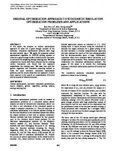
Figure 1. Annual invasions of brown plant hoppers (BPH) in southeast ASIA.

Figure 1 shows a map of the yearly BPH/WBPH invasions in Asia. In the Mekong Delta, the threat is essentially caused by BPH. And in fact, the plant protection centers encounter many difficulties in controlling this insect because of its complex dynamics. Firstly, the BPH life cycle is rather short with three stages: egg, nymph, and adult [6] [7] [15]. This insect can reproduce not only on rice but also on some other kinds of grass. Secondly, BPHs can migrate following the dominant winds to find their food sources [17] [18]. Several studies made by Otuka in 2009 noted that they can migrate on a very large spatial scale [4] [17]. To efficiently monitor the distribution of BPH, as we have already said before, and following a large invasion in 2005, a surveillance network with more than 300 light-traps has been established in 2006 in the Vietnamese Mekong Delta to help the managers 3

Chapter 1 ‒ Introduction recording the densities of adult insect on a daily basis. The initial intention was to build a systematic sampling network, where one light-trap (or several ones) would be considered as the representative(s) for one district (subdivision of provinces). This network has proved its interest in capturing data like the diversity of insects and can monitor the densities of about twenty different insect species. However, its main weakness lies in the spatial sparsity of the collected data, which causes a high variance of all statistical estimations undertaken (e.g., Kriging estimation [19][20]). Characteristics of the light-trap network

Figure 2. BPHs attack the

Figure 3. Insect surveillance network

young branches of rice.

in the Mekong Delta region.

The light-trap network established in the Mekong Delta has not evolved since 2006, since the location and sampling rate of each light-trap are fixed. There are actually several reasons for this stability: the availability of a power source nearby, the necessity to have trained personnel who are available, and some less obvious reasons due to the choices made by the management. Therefore, it cannot easily be adapted to changes of the environment (urbanization of areas, disappearance or appearance of rice fields, climatic changes) that may affect the spreading of BPH, and cannot easily be modified, except if these modifications are proved to improve its functioning on the long-term. Another characteristic of this network, and a difficult one to deal with, lies in the heterogeneity of the data collected, even between light-traps. Of course, the first reason lies in the weak density of the network, which can make each trap actually capture insects in very heterogeneous environmental conditions, but there are other explanations that are less obvious to take into account if we want to optimize it, such as human factors (e.g., keepers forgetting to inspect traps or report their result for several days, errors made in the manual reporting of the data, etc.). This is illustrated in Figure 4, which shows the mean trap-density of BPH collected by 48 light-traps in the year 2010.

4

Chapter 1 ‒ Introduction

Figure 4. Mean trap-density of BPH collected by 48 light-traps in 3 provinces: Hau Giang, Soc Trang and Bac Lieu in 2010.

In practice, then, as already said, the data collected by this network is not considered as reliable due to two main limitations: (1) low sampling density and (2) many impact factors are not taken into account. Therefore, the analysis and forecasting methods based on light-trap data are also less accurate.

a) Light-trap

b) Field monitoring frame

Figure 5. Recent studies and difficulties.

Prior to this research, a number of endeavors on optimizing the light-trap network have been undertaken by researchers at Can Tho University and SRPPC (the Southern Regional Plant Protection Center, owner and manager of the light-trap network). And several actual experiments have been done in dedicated case studies: (1) The setup of a denser network made-up of one light-trap per small town (subdivisions of district) in Tien Giang Province since 2010. (2) The setup of a dense network, coupled with the light traps, of field monitoring frames (about 120 frames / small town) in Trung An, Thot Not district, and Can Tho (operated in

5

Chapter 1 ‒ Introduction cooperation between Can Tho University and the Plant Protection Department of Can Tho in 2008) in order to capture the insects at different stages of their life-cycle [14]. (3) The setup of a hybrid network of light-traps and field monitoring frames in Hau Giang Province [13]. Another attempt at improving the usefulness of the network was done in the Vietnamese national project KC.01.15/06-10: “Design of Information Systems for supporting the Protection against Epidemic Diseases of crop plants and aquaculture in major economic areas”, developed by Can Tho University in coordinating with the SRPPC and the IRD/UMI UMMISCO [21]. In this project the researchers tried to increase the number of variables monitored by the existing network nodes in small towns of the Tien Giang and Dong Thap Provinces. Beside a number of specific thematic questions, the researchers principally ended up worrying about the performance of the network regarding the quality of the data and the difficulty to use it as an input for any prediction or estimation models. Their conclusion was that it was urgent to optimize the placement of the nodes so that the network could be used effectively for what it was intended to in the first place. However, establishing and maintaining a strategy that would consist in moving the nodes of the network from time to time in order to adapt it to the changes in the environment or to temporarily increase its density in highly infested areas, which is the most practical approach to solve the problems cited above, requires the mobilization of important financial resources, and the decision makers in charge of this network (mainly the SRPPC) are reluctant to take any decision in that direction until they can be convinced that this is the best one available.

1.3. Research questions and organization of manuscript Regarding to the available optimization approaches in environmental surveillance networks, the problem is that there are limited options available to convince decision makers: (1) practical experiments at small scales cannot be proved to remain successful at large scales and (2) theoretical works on network optimization neglect, for the most part, the internal or external factors that greatly affect the BPH populations, such as the farming habits, the use of pesticides, the variability of the weather, etc. The approach we propose in this manuscript is an attempt at overcoming the difficulties of the two approaches and at providing sufficient evidences to help the decision makers to make best decision over the future of the network. It is also a way to reconcile the theoretical and practical approaches, by (1) capturing in a model the richness of the complex system represented by the network and its ecosystem; (2) applying mostly theoretical optimization algorithms to simulations of this model in different realistic scenarios in order to find the best possible solutions for the placement of its nodes. Normally, optimizing such a network revolves around two main questions: (1) What would be the most appropriate density of traps?

6

Chapter 1 ‒ Introduction (2) What would be its most appropriate design, both in terms of placement and sampling rates of the traps? The difficulty of the first one is that, although it can be easily answered by some field experiments, these will be expensive to run and not so evident to generalize given the heterogeneity of the ecosystems composing the Mekong Delta. The second question raises other difficulties, which are usually addressed by optimization algorithms, among which the approaches known as optimal design [22] and metaheuristic optimization [23]–[25] are the most employed ones. The main difficulty of these approaches is that their performances can only be evaluated with respect to the existing sampling data, which is not always available in the real context. Furthermore, depending on the available data, these approaches may propose solutions that cannot be applied by the managers of the network. On one hand, if the data is too dense, the algorithms often try to remove several sampling locations or to decrease the sampling frequency in order to save costs. But, this solution, which might well be adapted for past sampling data, is potentially harmful regarding future situations, as the density of insects can be affected by human impacts (e.g., using pesticides, fertilizers and seed sowing by farmers [26][27]) or other causes that these algorithms do not take into account. On the other hand, if data is missing, these algorithms often deal with a high uncertainty in their estimations. This second problem appears more often than the first one, and additional optimization can be proposed to resolve it, but the lack of empirical data is clearly the main weakness of the traditional use of optimization algorithms. Finding a methodology that would enable deciders and experts to assess these “optimal” solutions in different scenarios, using both forecasted data and estimations of missing data, is the main purpose of this research, as the development of modeling and simulation techniques provides us with an opportunity to build virtual environments in which we can experimentally verify and assess the efficiency of potential network layouts. This research is therefore divided into five main topics: 1) Proposing a set of quantitative criteria to evaluate the performance of an environmental surveillance network. 2) Designing a virtual laboratory that couples a model of the surveillance network with one or more models of the environment. 3) Designing a set of optimization algorithms that can operate at different levels of representation of the simulated network. 4) Measuring the performances of these optimization algorithms in simulations against a handful of scenarios of growth and propagation of BPH. 5) Generalizing the approach for other environmental surveillance networks.

7

Chapter 1 ‒ Introduction The two first chapters constitute the general introduction of the thesis. In Chapter 2, we provide more information about NOVEL: How it is built and its theoretical foundations in both modeling and optimization. In Chapter 3, we introduce the design and the implementation of the laboratory, with a special attention to the components needed to reconstruct a realistic virtual environment. Chapter 4 presents three different scales of network optimization: micro-, meso- and macro-scale approaches. For each scale, we detail how it is implemented in NOVEL and how it is bound to be experimented within it. Chapter 5 contains the most important contribution of this thesis. In this chapter, we introduce some objective indicators in order to evaluate the performance of the surveillance network in NOVEL. This contribution is then shown to provide a useful support for all the users whether or not they want to assess a network inside or outside NOVEL. Finally, the general steps required to generalize NOVEL to related research domains are exposed in Chapter 6. We believe that our methodological proposal can be easily generalized and we show how, taking the examples from several domains. The conclusion and the future directions we intend to take are presented in Chapter 7. Figure 6 shows the organization of this thesis with all the chapters and their principal notions and links.

8

Chapter 1 ‒ Introduction

Chapters

CHAPTER 1. INTRODUCTION

CHAPTER 2. OBJECTIVES & STATE OF THE ART

Important notions & Links Brown Plant Hopper (BPH) (Section 1.1) Light-trap network (Section 1.2)

Complex multi-scale models (Section 2.1) Virtual laboratory (Section 2.4) Variogram & Estimation techniques (Section 2.7) Optimization methods (Section 2.8)

CHAPTER 3. NETWORK OPTIMIZATION VIRTUAL ENVIRONMENT LABORATORY (NOVEL)

Ecological Models (EMs) (Section 3.2) Model of the light-trap Network (Section 3.3) Disjointed Surveillance Network (DSN) [3.3.1] Correlated & Disk graph-based Surveillance Network (CDSN) [3.3.2]

CHAPTER 4. MULTIPLE SCALES OPTIMIZATION

Micro-scale optimization (Section 4.4) Meso-scale optimization (Section 4.5) Macro-scale optimization (Section 4.6) Root mean square error of variogram model (Section 5.3.1)

CHAPTER 5. EXPERIMENTAL ASSESSMENTS

Deviation of cross-validation (Section 5.3.2) Mean universal Kriging variance (MUKV) (Section 5.3.3) Aggregated indicators (Section 5.3.4) Ecological Models (EMs) (Section 6.1.2.1)

CHAPTER 6. METHODOLOGICAL PROPOSAL

Surveillance network model (SNM) (Section 6.1.2.2) Optimizers (Section 6.1.2.3) Evaluators (Section 6.1.2.4)

CHAPTER 7. CONCLUSION AND PERSPECTIVES

Figure 6. Thesis organization.

9

Chapter 2 ‒ Objectives and State of the art

CHAPTER 2

OBJECTIVES AND STATE OF THE ART

Chapter 2 gives a simple introduction to the contribution of the thesis, a virtual laboratory for network optimization. We try to define the main components of the laboratory, the most important properties of these components and to understand which previous studies can be reused and which ones have to be completely redesigned to handle these properties. Different states of the art are then presented, on agent-based models, Gaussian processes, as well as in network optimization, centered on two widely used approaches: optimal design [22] [28] and metaheuristic solutions [23]–[25].

2.1. Complexity and scales As mentioned in Chapter 1, building a virtual laboratory is the approach we have chosen to address surveillance network optimization. However, it relies on the possibility to reproduce, in silico, a part of reality that at least includes the interactions between the insects, their environment, and the surveillance network. This kind of integrated model, considered as a whole, belongs to the class of complex multi-scale models [29]. In this approach to modeling, the relationships between the different parts of a system are represented in all their richness so as to keep most of their significant “natural” properties and relationships. The drawback of this approach is that it often requires a large amount of multidisciplinary knowledge. It has however already been applied with success in numerous research domains, for example in ecology by Grimm et al. [30], economy by Anderson et al. [31], or social sciences by JASSS [32], and it is beginning to be considered as an interesting approach in environmental management by Paegelow [33] and by Wainwright [34]. 10

Chapter 2 ‒ Objectives and State of the art “Multiscale” is a concept used to divide the different levels observed in a complex system [35] [36]. The meaning of these scales strongly depends on the point of view of the observers. When it comes to modeling, however, the classification of these scales helps modelers to better control the complexity of their models, by defining the properties of each scale in isolation and focusing only on the interaction and data transmission between scales. It also allows them to handle situations where both local and global viewpoints on a phenomenon are needed: for instance, BPH migration will depend on local factors (availability of rice fields, interaction of the groups with pesticides, etc.) but will also obey global rules, for example by following the dominant winds. In a multi-scale complex systems approach, both viewpoints can be described, as well as their relationships. Not all modeling paradigms and techniques allow for a multi-scale representation of a complex system. The figure below shows that analytical models (based on a mathematical representation) are more adapted to representing macro-scales, where agent-based models (ABM) appear to be quite versatile but limited in terms of representing local and global dynamics and entities simultaneously.

Figure 7. Appropriate modeling methods for different scales of simulation domains (Course of “Complex systems” of Edith Perrier, IRD/France).

These limitations of ABM have actually never been conceptual, but mainly due to the limitations of the toolkits and platforms (NetLogo [37], Swarm [38], Repast [39]) supporting this kind of modeling. Recent developments in the domain have proved that ABM is now the approach of choice for supporting arbitrary levels of representation when modeling complex systems. A good example of this new trend can for example be found in the evolution of the GAMA agent-based modeling and simulation platform [36] [40] [41].

2.2. Modeling and simulating the whole system The claim that we can study how to optimize the surveillance network using a virtual laboratory is based on the availability of reliable modeling and simulation techniques of the complex system formed by the network and the other components of the real 11

Chapter 2 ‒ Objectives and State of the art system. Choosing the appropriate modeling and simulation techniques and the appropriate way of coupling them is then an important question, which will directly affect the quality of the results we will obtain. We do not try, in this research, to replace existing optimization methods (e.g., optimal design [22] or sampling techniques [42][43]), but to provide the most appropriate tool to apply and validate these methods in a virtual environment. Three main models seem at first necessary to support our needs: a model of the environmental processes that affect BPH propagation (which include climatic aspects, land-use processes, agricultural submodels, etc.); a model of the BPH themselves, which needs to include at least the life-cycle and migration processes of the insects; and a model of the surveillance network itself, so that it could be easily assessed and optimized in various scenarios. To simplify their presentation, we will categorize them into two main subsets of models: Models of the ecosystem: The ecosystem here represents all the components of the real system that are not directly related to the network: environment, insects, climatic conditions, human activity, etc. The most difficult part is of course the models dealing with the BPH migrations. Some typical models of time-series prediction can be found in [44], which use traditional algorithms like ARMA (AutoRegressive Moving Average) or ARIMA (AutoRegressive Integrated Moving Average), or by solving ordinary/partial differential equations (models of prey/predator [45], SIR model [46] [47] or growth models [7] [48]). Other approaches deal with the propagation of species in the specific study regions, such as the multifractal model for spatial variation in species richness [49], agent-based models of BPH propagation [50] [51]. In this thesis, the virtual environment contains a coupled model between two main submodels: BPH Growth Model and BPH Migration Model, which will be detailed in Chapter 3. Model of the surveillance network: The light-trap network is modeled as a multi-scale agent-based model that operates synchronously with the aforementioned ecological model and acts as a “virtual observer” of this model. The data obtained from its simulation can then be used for two purposes: (1) verifying, against historical data, the validity of the model of the ecosystem and (2) evaluating the performances of different network optimization strategies. It is enriched with internal operations on statistical criteria, especially geostatistical ones [19] [52] [53]. In order to remain as close as possible to realistic observation activities, we will define the observation process of the surveillance network as a true sampling process and use the vocabulary and methods described by Fisher [42] to conduct experiments. The sampling process will then monitor one or multiple observed variable(s) to provide simulated experimental data for end users, and these data will become the input of different analyses: population estimation, variable forecasting [54], etc. Building these different models raises several challenges, like the gathering of relevant data, but also intrinsic difficulties related to their inherent properties. We review several studies on these difficulties in the sections below. 12

Chapter 2 ‒ Objectives and State of the art The data gathered from the light-trap network are used in different stages of modeling and simulation in this thesis. This data source forms a set where each light-trap provides a time series data of insect trap-density. In this thesis, we use the notion of “trap-density” to specify the quantity of a specific insect type captured by the light-trap during a sampling cycle. Some other important data sources are also implemented in the laboratory, such as land-use data (especially agricultural land-use), weather data, e.g., temperature and humidity data, obtained from the meteorological stations and aggregated at the regional level (cf. [55][56] for aggregation methods), administrative boundaries data, and the GIS data of rivers and coastal regions of the Mekong Delta. In conclusion, our main research question is to design a decision-support system that allows decision-makers to simultaneously explore different layouts of the light-trap network in order to optimize its performances and to assess “optimal” configurations in different scenarios: BPH patterns, weather, etc.

2.3. Difficulties related to insect population modeling Since our research is to be validated on Brown Plant Hopper (Nilaparvata lugens (Stål)) invasions, we will essentially review the difficulties raised by this particular species for plant protection activities [6], without really taking into account the biotic heterogeneity [57] that characterizes insect populations in the region. However, the properties of this species listed below, such as randomness or autocorrelation, spatial dispersion or nonergodicity (in time), or its vulnerability to multiple impacts, are not specific to BPH and can be found in other species. 2.3.1. Randomness vs. Autocorrelation Randomness and autocorrelation are two opposite properties of the natural system we model in this research, which will partly decide which techniques or approaches can be employed to study it. Randomness The Oxford English Dictionary defines “random” as “Having no definite aim or purpose; not sent or guided in a particular direction; made, done, occurring, etc., without method or conscious choice; haphazard.” This concept of randomness suggests a non-order or non-coherence in a sequence of symbols or steps, so that there is no intelligible pattern or combination. Regarding light-trap data, the number of insects trapped every night is never totally random, but need to be considered as such. One of the reasons is that the limitation of the surveillance network hides the cause of their appearance at a given location: for example, the network cannot monitor the number of eggs or nymphs because these individuals cannot fly, but if we knew this number, we could probably forecast the number of insects that would be trapped. That is the reason why we need to consider this information as a random variable. And since the number of insects is a random variable, their dynamics can be considered as a random process.

13

Chapter 2 ‒ Objectives and State of the art Of course, if the numbers were completely random, the surveillance network would become useless and there would be no point in trying to optimize it. There are patterns like in every natural “random processes”, where several hyperparameters can be used to predict the values at unknown locations. Well known random processes include: •

Discrete time processes: Bernoulli processes, Markov chains, etc.

•

Continuous time processes: Cox, Lévy, Poisson processes, etc.

•

Mixed discrete & continuous time processes: Gaussian [58], Markov processes [59], etc.

Assimilating insect distribution and spreading to a Gaussian process is one of the main assumptions of this research, which leads us to use the Kriging estimation [19] [20] (or Gaussian process regression) in a number of algorithms, such as insect density estimation, or in some strategies of network optimization. As we will see in this work, autocorrelation is present in the trap network, and is at the heart of the possibility to use techniques such as Kriging evaluation since, without any local correlation, it would be impossible to pretend optimizing the network. Autocorrelation The correlation between two different quantities is normally used as a measure of their similarity [60]. In the surveillance data, the cross-correlation [61] between two different surveillance locations or the autocorrelation at one location directly affects the performance of the network. Both time series analyses (e.g., ARMA) and spatial analyses (e.g., Kriging) try to study the similarity of different time lags (e.g., ACF) or distance lags (e.g., variogram) for their prediction functions [52]. 2.3.2. Spatial dispersion and nonergodicity While the term of “spatial dispersion” describes the difference and the irregularity of the density of insects in space, “nonergodicity” describes them in time. These two properties partly reflect the complexity of the ecosystem. The spatio-temporal changes of the insect ecosystem strongly depend on multiple natural and human factors, some of them being difficultly controllable (e.g., climate change, land use, pesticide use, etc.). These heterogeneous factors affect the natural distribution of insects, and consequently the stability of the surveillance network. Hence, in some circumstances, the surveillance network can become completely ineffective. For instance, in the Mekong Delta, some provinces have stopped the maintenance of light-trap network because of the changes in land use (like Ca Mau following the extension of aquaculture activities). More explanations regarding these two concepts are shortly introduced as follows: Spatial dispersion Figure 8 shows the contour plots of two surfaces where the relief of Surface 1 seems significantly rougher than one of Surface 2.

14

Chapter 2 ‒ Objectives and State of the art

a) Surface 1

b) Surface 2

Figure 8. Two different dispersion data (Source [62]).

The histogram analyses of these two surfaces are given in Figure 9. We cannot find a big difference between these two histograms, whereas their variograms (variance diagrams) in Figure 10 show a clearer difference.

a) Histogram of surface 1

b) Histogram of surface 2

Figure 9. Histograms of two different dispersion data (Source [62]).

In Figure 10, the left variogram shows a strong increase of variance in the range from 0 to 15 units of lag distance, whereas the right one shows a slower change of variance.

15

Chapter 2 ‒ Objectives and State of the art

a) Semivariogram of surface 1

b) Semivariogram of surface 2

Figure 10. Variograms of two different dispersion data (Source [62]).

These figures show that empirical variograms can be used to provide relevant insights about spatial dispersion. Evaluating the regression model of variograms is already an important method to assess the performance of a surveillance network. If a network has a low sampling density and does not satisfy the Nyquist–Shannon condition [43] [63] regarding sampling density, it will be impossible to propose a good regression model, without too much errors, based on its variogram. Conversely, the errors in the regression model can become a quantitative indicator to assess the performance of this network. Nonergodicity

Figure 11. Standardized residuals (Trap-density data at Dai Thanh, Nga Bay Town, Hau Giang Province, Vietnam).

Figure 11 shows an example of standardized residuals for trap-density data for one year. These time series data have been collected during 365 days in 2010 at Dai Thanh, Nga Bay town, Hau Giang province, Vietnam. 16

Chapter 2 ‒ Objectives and State of the art

Figure 12. Time series prediction by ARIMA (Trap-density data at Dai Thanh, Nga Bay Town, Hau Giang Province).

Figure 12 shows an ARIMA prediction for the same time series data. The blue line draws the predicted values for the following 40 days. The red and green lines show the standard deviations around these predicted values. Such analyses could be useful in two tasks of this research: (1) in predicting the outcomes of the growth model of insects and (2) in becoming a criterion during the verification of the predictions made by simulation. However, this approach is not completely effective with high values of standardized residuals, at some points in time, as presented in Figure 12, which means that the time series data are nonergodic. 2.3.3. Heterogeneity Many extrinsic factors can disrupt the natural distribution of insects. These factors can be caused by natural or human processes and are called the “nuisance parameters” of the prediction models. Some of these factors will be considered in this research: • • •

Natural factors: temperature, humidity, wind (direction and speed). Biological factors: predators and parasitoids of insect. Human factors: land use planning, cultivation planning.

17

Chapter 2 ‒ Objectives and State of the art

a) Adopting 3R3G in An Giang Province from 2002 to 2008. (Data source: An Giang Department of Agriculture, Long Xuyen, Vietnam).

b) Poster for “Three Reductions, Three Gains” program [27].

Figure 13. Scaling out communication to rural farmers: lessons from the “Three Reductions, Three Gains” campaign in Vietnam [27].

For example, in Vietnam, a large campaign named “Three Reductions, Three Gains”, launched in 2001, tried to convince the farmers to follow the strategies proposed by agricultural experts in using different rice seeds, less fertilizers and less pesticides [27]. Figure 13 shows the adoption rates of these strategies by farmers in An Giang Province from 2001 to 2008 and one typical poster for this campaign. We clearly see here that the human impacts on the insect population can become extremely important if coordinated behaviors are put into practice. This campaign demonstrated several successes, but the BPH adapted and their invasions, although different in shape and nature, are still very difficult to control. Multiple factors like this one are known to directly affect the heterogeneity, spatial dispersion and spreading of BPH populations.

2.4. How to build the virtual laboratory (NOVEL)? Determining the necessary components of NOVEL to support various virtual experiments is the central question of this thesis. Even without precisely knowing the range of virtual experiments that need to be performed, we have to choose an appropriate approach, including the techniques, services, or platforms, etc., that can support modeling, coupling and combining separate functional components. Besides this, it is also required that these models, which will be used to simulate reality and generate simulation data, be as realistic as possible. The satisfaction of this requirement ensures that the outcome of virtual experiments can be verified and furthermore, that the solutions proposed, e.g. potential network layouts, can be possibly applied.

18

Chapter 2 ‒ Objectives and State of the art 2.4.1. Components of NOVEL In order to ensure this requirement of realism, we need to rely on the context and the data sources available, especially on the structure and operation of the existing lighttrap network (cf. Figure 3). In Section 2.2, we suggest that two groups of models need to be developped and coupled: (1) models of the ecosystem and (2) model of the surveillance network. Obviously, the important properties of BPH populations that have been identified in Section 2.3 must also be present in NOVEL. Virtual Ecology, initially proposed by Grimm et al. in 1999 [64] and refined by Zurell et al. in 2010 [65], proposes to model ecological surveillance tasks using a framework composed of four main components: (1) A virtual ecological model, which produces data, (2) A virtual sampling model, which observes the data, (3) Statistical models to build inferences on the data, and (4) Evaluation models to compare produced and real data. Our proposal for components of NOVEL is based on this approach, but in our case, the goal is to “infer” and assess optimal network layouts. Thus, a system of 4 components is proposed in NOVEL: (1) Ecological models, (2) Model of the light-trap network, (3) Optimization processes, and (4) Assessment processes.

Figure 14. Abstract view of NOVEL.

Figure 14 shows an abstract view of NOVEL with all 4 sub-systems and its internal data flows: 1) “Ecological Models”: This component, which mostly contains models and is responsible for the simulations of the BPH invasions in different scenarios, groups all the factors related to the dynamics of BPH, including food sources (rice-cultivated regions), the weather or the obstacles like rivers/seas, growth and migration models. 19

Chapter 2 ‒ Objectives and State of the art All these models are spatially coupled: a cellular automaton is used to model the study region as a lattice of rectangle cells; each cell contains the local information regarding the environmental and biological system it belongs to and is used as a common structure for the coupling between the models. This sub-system will be extensively covered in Chapter 3. 2) “Model of the Light-trap Network”: This sub-system contains and manages the model of the surveillance network, i.e. light-trap network. This model is used to monitor some variables supplied by the cellular automaton of the previous sub-system and is directly manipulated (and possibly modified) by the components of “Optimization Processes”. 3) “Optimization Processes”: Multiple optimization algorithms are implemented to explore different layouts of the light-trap network in order to optimize its performances. 4) “Assessment Processes”: Various indicators assess its performances and serve as the criteria to assess “optimal” configurations in different scenarios (e.g. BPH patterns, weather). It is clear, from this figure, that the “Model of the Light-trap Network” sub-system is a central component of the whole system. As a matter of fact, it plays three roles at once: 1) With respect to the ecological and environmental models, it plays a role of “perception component” of the whole system they form, borrowing information from it as a real network would do. This task is represented by the monitors() relationship on the figure (which will directly translate into the behavior of some components of the model). 2) From the point of view of the “Optimization Processes” sub-system, it must provide a flexible interface to support the re-organization of the network modeled, allowing for the addition or deletion of measuring devices or the reorganization of their locations and frequencies. This task is represented by the optimizes() relationship. 3) Finally, it needs to reflect the actual surveillance network, with respect to both its organization and its operations, as faithfully as possible, so that decision makers can easily translate lessons learned in simulations to possible actions in reality. 2.4.2. Which approach can be used? Choosing the technique(s) that can Definition. Agent-based model (ABM), presented by Gilbert [70]. support representing the various Agent-based modeling (ABM) (...) involves building a computational models built for NOVEL (including model consisting of agents, each of which represents an actor in the their various properties and local social world, and an “environment” in which the agents act. Agents are able to interact with each other and are programmed to be proconstraints) is not an easy task. In active, autonomous and able to perceive their virtual world. The fact, there are multiple relations at techniques of ABM are derived from artificial intelligence and computer science, but are now being developed independently in different scales that need to be research centers throughout the world. considered at the same time: the spatial estimation [66], the models of the growth process [7], human impacts [27], ecological impacts [67], survey activities by light-traps [11] [63], etc. Moreover, in case of BPHs, some remarkable properties, such as their heterogeneity or dispersion, should be thoroughly noted, in order to conduct virtual experiments at different scales [35]. 20

Chapter 2 ‒ Objectives and State of the art Moreover, and besides the difficulties of building individual models, integrating and coupling all the necessary models require a conceptual and operational modeling framework that can support different techniques, different scales, and different point of views. Agent-based modeling (ABM) [68]–[70], in that respect, appears as an appropriate technique for this purpose. A review of the recent research on individual-based models, agent-based models and multi-agent systems underlines the fact that ABMs are increasingly used in noncomputing related scientific domains including Life Sciences, Ecological Sciences and Social Sciences [69], precisely because of their versatility and capabilities in coupling different techniques, at different scales of space and time. Furthermore, it has been shown that particular optimization techniques, such as Tabu search [71] or Particle Swarm Optimization (PSO) [72]–[74] are very well adapted to the representation used in agent-based models. The core of NOVEL will then be based on an ABM meta-model, implemented on the GAMA platform. GAMA [38] [70] [71] has been chosen because of many interesting characteristics: •

• • •

The possibility to easily couple and combine different models, possibly written using other modeling concepts (ODE, PDE, Cellular Automata, Dynamic Systems). Its inherent support of multiple-scale models, through the implementation of nested models and its explicit definitions of spatial and temporal scales. Its support of GIS data (read/write from/into distributed spatial RDBMS). Some advanced features like the management of multiple topologies (graphs, lattices), a tight interaction with the R language [77] and sophisticated 3D visualization.

GAMA is being developed since 2007 by a set of partner laboratories, cooperation between France and Vietnam (IRD/UMMISCO1, IFI/MSI2, CTU/DREAM3, UT1/IRIT4, P11/LRI5, Rouen/IDEES6), which has allowed us to benefit from direct interactions with its developers. A PhD student has also contributed to the platform during this research, namely by designing and implementing the interaction with the R environment.

2.5. How to couple the submodels? The basic “bricks” for building NOVEL are now more or less determined, including the important properties of the BPH ecosystem (cf. Section 2.3), its main components and the appropriate approach, i.e., ABM (cf. Section 2.4). However, we also need a general design that can give answers to the following questions:

1

www.ummisco.ird.fr www.ifi.auf.org/site/content/view/35/46/ 3 http://www.ctu.edu.vn/dream/ 4 http://www.irit.fr/ 5 https://www.lri.fr/ 6 www.umr-idees.fr 2

21

Chapter 2 ‒ Objectives and State of the art (1) How to initialize models using the input data, for example, the BPH trap-density data, the data related to different local or global constraints, etc., given that these data have been collected and are represented at very different scales? (2) How to represent the monitors() task of Figure 14? And how to ensure that this task is realistic enough compared to what happens in reality? (3) How to represent the optimizes() task (i.e., the placement of the light-traps) of Figure 14? How can this interaction be automatically performed inside the laboratory? To answer these three questions, we need to clarify in which way the submodels can be coupled with each other although they are situated at different scales. We do not have the intention to propose a detailed design of the laboratory in this section, but to only focus on the general directions we have chosen for its implementation, which will be presented in Chapter 3. The main choice we have made is to use the smallest temporal and spatial scales available in our data in order to synchronize and couple all the models on them. With such a choice, models and their components are able to easily interact with any other object at similar or higher levels. 2.5.1. Spatial coupling For example, while a light-trap is managed at the administrative scale of a small town/district, it can represent a very small space in the study region, so the discretization of the space appears necessary. In ABM, cellular automata is often considered as the most interesting choice to represent both the spatial discretization and the interactions between the spaces, while allowing these spatial units to interact with agents at higher levels (the light-traps and their zones of influence, such as the rice-cultivated areas or administrative regions, etc.) The first cellular automaton Definition. Cellular automata, presented by Wolfram [79]. (CA) was first developed in Cellular automata are mathematical idealizations of physical systems in which the 1940s by Stanislaw space and time are discrete, and physical quantities take on a finite set of Ulam, who was discrete values. A cellular automaton consists of a regular uniform lattice (or “array”), usually infinite in extent, with a discrete variable at each site (“cell”). investigating the growth of The state of a cellular automaton is completely specified by the values of the crystals, and by John Von variables at each site. A cellular automaton evolves in discrete time steps, with the value of the variable at one site being affected by the values of variables at Neumann, who was working sites in its “neighborhood” on the previous time step. They have been applied on the problem of self- and reintroduced for a wide variety of purposes, and referred to by a variety of names, including “tessellation automata”, “homogeneous structures”, “cellular replicating systems [78]. structures”, “tessellation structures”, and “iterative arrays”. This technique is now mainly used for representing the dynamics of different kinds of environments [79]–[81]. In its detailed study of the class of CA based models, Wolfram underlined that “even when the underlying rules are very simple, the behavior they produce can be highly complex, and can mimic many features of what we see in nature” [81]. Synchronous and asynchronous updates are the two main methods applied in cellular automata. Asynchronous methods in which the time variable is not explicitly defined, operate by specifying an updating order of the cells [80]. In the synchronous method, the variables at each site are updated simultaneously, based on the values of the variables in their neighborhood at the preceding time step, and according to a definite 22

Chapter 2 ‒ Objectives and State of the art set of “local rules” [79]. We apply two cellular automata as the main solution to couple multiple submodels at different spatial scales in NOVEL (cf. Figure 17), all of them are essentially updated by the synchronous method. 2.5.2. Temporal coupling Our meteorological data of the meteorological stations are produced on a monthly basis, while the trap-density data are produced daily, (See MARD7 ‒ Meteorological Data by Month, Years, and Stations, Ministry of Agriculture and Rural Development). In our model, we logically chose the day as the lowest scale applied for the models. One day will then correspond to one step in the simulation.

2.6. How to model the BPH trap-density data? The properties of the distribution of BPH in a spatio-temporal zone, namely randomness and autocorrelation, have already been indicated. The question is how to model this distribution in our model(s), and more concretely, how to map it to an environment based on a cellular automata representation. As aforementioned, cellular automata are often used to model spatial zones, their dynamics and interactions. Regarding time, as mentioned in Section 2.3, there are two representations that are probably adaptable to model both the discrete and continuous time processes, respectively Gaussian processes [58] and Markov processes [59]. It should be noted that both discrete and continuous time processes are necessary to be considered in our work, as they correspond to the need to exchange data between the real environment (i.e., in reality) and the discrete environment (i.e., the collected and simulation-produced data). Both models are therefore intentionally used in NOVEL; Gaussian processes are used to support the estimation of BPH trap-densities in a specific study region, while Markov processes support the dynamics of the models, essentially for the BPH growth and migration models. Because Markov processes are rather easy to understand, and because their implementation is covered in Chapter 3, we will just provide in the following sections some bases about Gaussian Processes. 2.6.1. How are the BPH trap-density data modeled? As already mentioned, we need to manage different data sets with different characteristics, inside our virtual environment: the data collected and the data produced by the simulation itself; both will be named “sampling data” in the following. Sampling data are defined as the data collected from multiple sampling devices (or measuring devices) of a network. Normally, these data are analyzed by statistical techniques to estimate the population of concerned variables. In our research, the sampling data are considered as a realization of a Gaussian process [90] [91]. Three important charasteristics of sampling data are their spatial, temporal, and multivariate traits. A definition of a spatio-temporal random field is given below:

7

http://fsiu.mard.gov.vn/data/khituong.htm

23

Chapter 2 ‒ Objectives and State of the art Definition. Spatio-temporal random field. A spatio-temporal random field F is a stochastic process denoted by

where

=

and

( , )|

∈

,

∈ ,

⊂

,

⊂ }

respectively denote the space area and the time duration,

(1)

( , )

denotes the value of random variable at a specific continous space-time point (s, t). Concretely, a sampling design is developed by the end users to monitor the status of a random field F at some specific time and space scales. Sampling data are considered as the realization of F, and it must be a subset of F.

Cressie presented the statistical spatio-temporal model in [52], which is also our approach in this thesis. Supposing that Z is the sampling data of a random field F, Z is defined as the following: ( , )=

where

,

|

∈ ,

∈ ,

≤ ≤ !,

≤ ≤ "#

(2)

s and t denote respectively the space and time of sampling, n denotes the number of sampling sites, m denotes the sampling times. $, %

denotes the observed value of random variable at a specific

sampling point

$, %

.

Although the data model of F is not defined yet, where Z(s, t) is a representative of F, F can have the same model in Equation 2 without any limit on m and n. Using this data model, we can explore some intrinsic relations inside F by a number of covariance functions and some approximation techniques applied on Z(s, t). 2.6.2. Gaussian process With the assumption of a random Definition. Gaussian process, defined by Rasmussen in 2006 [82]. field, the variable concerned at a A Gaussian process is a collection of random variables, any finite specific spatial site s will be an number of which has a joint Gaussian distribution. independent random variable, denoted as Z(s). In addition, since we assume that F is a Gaussian process, not only the variables but also the covariance functions will be Gaussian processes. A Gaussian process is completely specified by its mean function and covariance function. We define the mean function m(x) and the covariance k(x, x’) of a process as: !(&) = '[)(&)] 24

(3)

Chapter 2 ‒ Objectives and State of the art +(&, &’) = '[()(&) – !(&)) ()(&’) – !(&’))]

(4)

)(&) ~ /0(!(&), +(&, &’))

(5)

and hence, a Gaussian process will be written as:

A Gaussian process is a generalization of the Gaussian probability distribution. While a probability distribution describes random variables (scalar or vector), a stochastic process governs the properties of functions. We denote a random function 1 ~ 23(μ, 5), i.e, the random function f is distributed as a Gaussian process with mean function µ and covariance function K. In the case of Kriging estimation (cf. Section 2.7.1), also known as Gaussian process regression (GPR) [20] [82], 5 = 6( 7 , 8 ) = 9:;( 7 − 8 ) is used as a covariance function. The mean function µ can also be equal to 0 (Simple Kriging), or to a constant mean value µ0 (Ordinary Kriging).

2.7. How to estimate the BPH trap-densities of unmeasured locations? Estimation techniques are classified into two groups: deterministic solutions (polynomial interpolation [84], radial basis function (RBF) [85]) and stochastic solutions (Kriging estimation [20] [19] and Bayesian inference [86]). In this research, we essentially concentrate on a stochastic solution in which the Kriging interpolation is the main approach. Kriging is the principal technique mentioned in geostatistics. It has first been applied in mineral mining related researches, but is now used in a wide range of applications. 2.7.1. Kriging estimation Geostatistics [19] is a branch of statistics that especially focuses on spatial analysis instead of spatio-temporal analysis [52]. Kriging (named after Krige, and developed by Matheron [19]) is a popular interpolation method to estimate the values of variables observed at unknown locations from some sampling data set. Nowadays, this technique is not used only in geostatistics anymore, but also in different communities such as environmental sciences, hydrogeology, natural resources management, etc. Multiple kinds of Kriging methods exist, depending on the assumptions they make about the environment (or random field). Simple Kriging (SK) has an assumption of a known mean value, while Ordinary Kriging (OK) requires only a constant mean condition (but unknown). More generally, Universal Kriging (UK) considers that the random field has a non-constant mean value. Ripley, in 1981, and Cressie, in 1993, gave a thorough analysis of Kriging methods in spatial statistics [20] [87]. In the different Kriging methods, the establishment of a variogram is considered as a central factor. Thanks to its approximation function (cf. the variogram model mentioned below) mean values and variances of unmeasured locations can be computed. Variograms were introduced by Matheron in 1963 [19]. It should be noted that early papers by Kolmogorov in 1941 (as the structure function [88]) and by Jowett in 1952 (as the mean-squared difference [89]) defined the variogram in one dimension [52]. 25

Chapter 2 ‒ Objectives and State of the art In spatial statistics, variograms exist in two different varieties: theoretical and empirical ones. Theoretical variogram A theoretical variogram 2γ(x,y) is a function describing the degree of spatial dependence of a stochastic process (such as Gaussian process [82]). =(&, >) = ?@A

(&) −

(>) = '(B

(&) − C(&) − ( (>) − C(>))B )

(6)

In case of a constant mean μ of the stochastic process, the expression to calculate the variogram is the following:

=(&, >) = '(| (&) −

(>)| )

(7)

Empirical variogram Empirical variograms are defined in geostatistics as the first estimation of the theoretical variogram needed for spatial interpolation by Kriging technique. In spatial analysis, for observations zi, i = 1, 2, …, k at locations s1, s2, …, sk an empirical variogram, as defined in Cressie (1993), is:

D(E) = =

F |G(E)|

H B

( , )∈G(E)

−

B

(8)

where N(h) denotes the set of pairs of observations i, j. Generally an “approximate distance” h is implemented to represent a certain tolerance. In practice, the empirical variograms allow us to characterize the spatial smoothness or roughness of a data set. Variogram-based analysis consists in computing a from the data and building a variogram model fitted to this data. There are some popular variogram models that are often used: Linear model, Exponential model, Spherical model, Gaussian model and Matérn model. Each of them has a specific set of hyper-parameters that need to be tuned (or fitted) before they are applied. As mentioned before, we will use a feature of GAMA that allows to directly from within a simulation the gstat library [90] with a set of appropriate hyper-parameters from NOVEL. In Annex 3, several related code snippets are presented. 2.7.2. Noising and smoothing processes In practice, when applying the results of a Kriging estimation, we cannot rigidly apply the estimated mean values for all simulation times. Doing that would transform the status of simulation data from random to deterministic, and this clearly does not satisfy the inherent properties of the BPH trap-density data. Fortunately, Kriging methods provide us with an estimated variance, and this variance can be used as an added noise to the estimated mean value to increase its randomness. This technique is called “Gaussian noise”.

26

Chapter 2 ‒ Objectives and State of the art Gaussian noises are determined by the mean value and the variance of the Kriging estimation. A random noise based on the Gaussian variance is added to the mean value for each estimated location; the final value is called the Gaussian noise density. Gaussian noises help to generate various scenarios of the environment during the estimation process. In NOVEL, as will be presented in Chapter 3, Gaussian noise density is separately computed for every cell of the environmental cellular automaton. Thus, the differences of Gaussian noise densities between two adjacent cells can be high. These differences do not exist in a real context, which means that we also need to apply some smoothing process. Concretely, this “smoothing density” is computed by the mean value of all Gaussian noise densities of the cells’ neighbors. This is then used in place of the raw Gaussian noise density.

2.8. How to optimize the light-trap density network? 2.8.1. Quantifying the uncertainty of the estimated results Quantifying the uncertainty of the results obtained in our laboratory can be considered as a measure of the performance of the whole surveillance network based on a specific estimation technique. We will take advantage of this by the way of performance indicators described in Sections 5.3.2 and 5.3.3. It also provides a solid foundation for optimization strategies; in fact, all the optimization algorithms presented in Chapter 4 will be based on this quantification (or similar ones), where the basic idea will be to install new light traps in locations with high uncertainty level; and in the opposite case, to remove existing light-traps from the network if this removal does not strongly affect the accuracy of the whole network. In each particular algorithm, several additional criteria will of course be considered. In the Kriging methods, an often-used measure of the uncertainty is called the Kriging variance. In this thesis, several measures of uncertainty are used based on the Universal Kriging estimation [20] [91], essentially the Universal Kriging variance (UKV). Furthermore, in Section 4.3.2, Universal Kriging Standard Error (UKSE) is mentioned as an alternative measure of UKV, and this approach is based on the so-called Gaussian process entropy (GPE). Gaussian process entropy (GPE) In information theory, entropy is a measure of the uncertainty associated with a random variable [92]. This notion has firstly been introduced by Shannon in 1948 [93]. In this thesis, the measure of the uncertainty is based on the Kriging estimation, and its variance is a form of entropy. Since Kriging estimation is also known as a Gaussian process regression [83], the entropy of Kriging estimation is the entropy of the Gaussian process (or Gaussian process entropy ‒ GPE).

27

Chapter 2 ‒ Objectives and State of the art

Figure 15. Estimated trap-densities by

Figure 16. Universal Kriging variances.

using Universal Kriging technique.

Figure 15 shows the estimated trap-densities in the study region by using UK, whereas Figure 16 shows the UK variances in the same context. The accuracy of estimation in this case is very low because the UK variance is too high. The farther the estimated locations are from the sampling locations, the greater Kriging variance is. This measure can for example lead greedy optimization approach, where new measuring devices would be installed at locations of high variance. 2.8.2. Typical optimization approaches Optimizing an environment surveillance network is the primary goal of this thesis. For several reasons mentioned above, we chose an approach based on simulation to solve this problem. The optimization process comprises two steps: (1) optimization itself of the surveillance network and (2) assessment of its performance. Conventional approaches can help in performing the first step. In our opinion, however, the second step plays a more important role and provides more detailed evidences for or against optimal network layouts. These two processes are installed inside two sub-systems called “Optimization Processes” and “Assessment Processes” (cf. Figure 14). Optimizing the surveillance network aims at proposing an optimal layout by adding, deleting or re-planning the location of measuring devices. Cross-validation, in many cases, can be applied for network optimization. As per this technique, each element is picked out of the training set and compared with its estimated/predicted value. Using cross-validation in optimization is suggested by Cressie (1993), namely using the deletion of a site from the network [20]. Thus, if a node has a serious error in crossvalidation, it becomes an important node and should not be removed from the network. Otherwise, if a node has a low error, it can be removed from the network. In our work, optimization algorithms will be classified into local search based algorithms (micro-scale), proximity search based ones (meso-scale) and global search based ones (macro-scale). As we will see in Section 4.1 of Chapter 4, this classification depends on the network organization that is defined inside NOVEL. 28

Chapter 2 ‒ Objectives and State of the art 2.8.2.1. Experimental design and optimal design Experimental design, or design of experiments ‒ DOE, is defined as a design of any information-gathering exercises where some variation is present depending on different experimental strategies [39] [80] [81]. Optimal designs are one class of DOE [22], which aims at proposing a sampling design with respect to several statistical criteria. This thesis examines a small class of experimental designs, the one concerned with environmental sampling, a technique important in many domains of environmental and ecological applications, such as agricultural management [11] [12], fishery surveillance [96], or forest management [40] [83]. Atkinson et al. thoroughly discussed optimum experimental designs based on a covariance matrix of the empirical data [22]. Numerous optimal designs are proposed as macro-scale strategies, such as A-, D- or E-optimal designs (applied on a covariance matrix) [9] [22]. 2.8.2.2. Metaheuristic optimization Metaheuristics are divided in two Definition. Metaheuristics, presented by Blum and Roli [24]. categories: trajectory-based Metaheuristics are high level concepts for exploring search spaces by metaheuristics that start with a using different strategies. These strategies should be chosen in such a that a dynamic balance is given between the exploitation of the single initial solution, and way accumulated search experience (which is commonly called population-based metaheuristics intensification) and the exploration of the search space (which is called diversification). This balance is necessary on one side where the initial population is commonly to quickly identify regions in the search space with high quality solutions randomly generated or created and on the other side not to waste too much time in regions of the space which are either already explored or don’t provide high with a greedy algorithm. All search quality solutions. metaheuristic algorithms in this thesis are population-based metaheuristics. Popular ones are Tabu search [71], Ant Colony Optimization [98] or the swarm optimization (e.g., Particle Swarm Optimization [72]). Although metaheuristics is a large class of algorithms that can provide solution for various problems, we will only use them to optimize the surveillance network, using what is called “metaheuristic optimization”. A recent survey of this trend can be found in [25]. Evolutionary algorithms (EA) An evolutionary algorithm is a generic population-based metaheuristic optimization algorithm. It uses some mechanisms inspired by biological evolution, such as reproduction, mutation, recombination, and selection. It is to be noted that agent-based approaches share similar characteristics with EA, and their combination, known as Agent-based Evolutionary Search (AES), proves to be an interesting approach in applications similar to ours [99]. For example, Yan and Sarker introduced an evolutionary approach into agent-based simulation, calling this “dynamic optimization” [99][100]. This combination is also applied in many other domains, for example to optimize the placement of evacuation signs on road networks in case of emergency [101] [102].

29

Chapter 2 ‒ Objectives and State of the art

2.9. Conclusion In conclusion, Chapter 2 presented the main objectives pertaining to this thesis. Based on the analyses of the studies that had been done to improve the performance of the light-trap network in the Mekong Delta, we showed that, besides the “technical restrictions” of using evolved optimization techniques, the “practical restrictions” in assessing optimal layouts constitute the biggest obstacle for decision makers in deciding how to change the network. However, we showed that, instead of applying an assessment based on real experiments, a solution based on simulation could also provide good evidences to evaluate network layouts before applying them in a real context. So, modeling the whole system, including the BPH ecosystem and the surveillance network, in order to deliver realistic simulations of potential network layouts, is the most important goal of this thesis. This is achieved by building a virtual laboratory that can support multiple network optimization algorithms and experimental assessments. An abstract view of this laboratory has been introduced, with three functional sub-systems: (1) Ecological & Environmental Models (EEMs), detailed in Section 3.2, (2) Surveillance Network Model (SNM) detailed in Section 3.3 and (3) Evaluation & Optimization Component (cf. Section 2.4). We showed that this abstract view opened a range of questions, most of them revolving around the problems of building the models, connecting these different components and choosing their mechanisms, etc. Corresponding to each question, possible solutions have been reviewed and a specific choice has been proposed, as follows: To build the models constituting NOVEL (cf. Section 2.1), we primarily chose an Agent-based modeling approach. To combine different models into a uniform system (cf. Section 2.5), NOVEL will support the lowest spatial and temporal scales of the data available. A CA-based technique is then proposed to combine the models at a spatial level, whereas the day is chosen as the smallest scale of time. To model the trap-density data (cf. Section 2.6), Gaussian and Markov processes are used to model the dynamics of this data. These two processes support both discrete and continuous data. To estimate the trap densities at unmeasured locations (cf. Section 2.7), a Kriging estimation (or Gaussian Process Regression), is proposed as an appropriate solution to represent the stochastic processes of this data. Finally, to optimize the light-trap network and assess its performances (cf. Section 2.8), two typical optimization techniques have been reviewed, and we will propose, in Chapter 4, some improved and novel approaches related to these two ones. The optimal layouts obtained this way will then be assessed inside NOVEL by using the simulated trap-density data.

30

Chapter 3 ‒ Network Optimization Virtual Environment Laboratory (NOVEL)

CHAPTER 3

NETWORK OPTIMIZATION VIRTUAL ENVIRONMENT LABORATORY (NOVEL)

Building a virtual laboratory, as mentioned in Section 2.4, is our approach to address surveillance network optimization. In this chapter, the implementation of this laboratory using an agent-based approach is mentioned in the context of light-trap networks. Almost all important factors of the real context are modeled, and divided into two groups: (1) Ecological Models (EMs) and (2) Model of the Light-trap Network. In this chapter, we essentially focus on the modeling process, but a verification process is also introduced to evaluate the accuracy of the BPH prediction model (i.e., the integrated model of EMs). Chapter 4 and 5 will respectively explain how to apply this laboratory for surveillance network optimization and experimental assessement of different potential network layouts.

3.1. Motivation This chapter is designed as a practical answer to some of the questions introduced in Chapter 2. In Figure 14, an abstract view of NOVEL has been presented, where four principal sub-systems are proposed: (1) Ecological Models (EMs) presented in Section 3.2, (2) Model of the Light-trap Network presented in Section 3.3 (3) Optimization Processes presented in Chapter 4 and (4) Assessment Processes presented in Chapter 5. All these components are integrated into NOVEL.

31

Chapter 3 ‒ Network Optimization Virtual Environment Laboratory (NOVEL)

Figure 17. General architecture of NOVEL.

Figure 17 graphically illustrates (1) how we employ cellular automata to model the ecological and environmental dynamics, and (2) how we represent the interaction between the surveillance network and its environment. Each cellular automaton is used to model the spatial environment as a lattice of cell agents. Each cell agent represents a separate rectangular zone in the study region. EEMs rely on two cellular automata. The first one is used to maintain the information on BPH’s stages/life-cycle, e.g., eggs, nymphs, adults, and, on the other hand, some environmental parameters, e.g., temperature, wind speed, land-use. A synchronous update is applied to this automaton. The second one (Heuristic cellular automaton) helps to maintain the information of UKSE (or a combinational heuristic argument as explained in detail in Section 4.3.2) that is primarily used to support the optimization algorithms (presented in detail in Chapter 4). This heuristic cellular automaton is just updated one time at the beginning of the optimization process. GAMA [38] [70] [71] supports a mechanism that allows implementing multiple cellular automata in parallel with other GIS-based agents. Therefore, in the scope of this thesis, all the models of the virtual labobatory are implemented on this platform.

3.2. Ecological Models 3.2.1. Requirements and solutions This section concentrates on the modeling process ‒ building all necessary models related to the ecosystem of BPHs using agents. The main goal of Ecological Models is to reproduce all the important properties of the real system listed in Section 2.1, which include: (1) Randomness & Autocorrelation, (2) Spatial dispersion & Nonergodicity, and (3) Heterogeneity. Section 3.2.2 presents all the entities needed to develop the models and couple them. Sections 3.2.3 and 3.2.4 respectively introduce two main groups of submodels: (1) Environmental submodels and (2) Biological submodels. All the submodels of these two groups are listed in Table 1. .

32

Chapter 3 ‒ Network Optimization Virtual Environment Laboratory (NOVEL) Table 1. Two main groups of submodels: Environmental and Biological submodels. Environmental submodels

Biological submodels

Objectives Modeling the nuisance factors that affect the dynamics of the population of insects Input data (1) Rice cultivated regions in two crop seasons: Summer-Autumn & Winter-Spring (2) Statistical weather data (meteorological stations): Temperature & Humidity (3) Statistical wind data (4) Sea and river regions Simulation step One MONTH Submodels (1) Temperature model (2) Humidity model (3) Wind model

Objectives Modeling and simulating the life-cycle and migration of insects Input data (1) Light-trap sampling data (2) Simulated wind data: Direction and Velocity

Simulation step One DAY Submodels (1) BPH growth model (2) BPH migration model

3.2.2. Entity specifications In this section, we provide the descriptions of all the agents installed in Ecological Models (see Figure 14). Components related to Model of the Light-trap Network will be mentioned in Chapter 4.

Figure 18. Three state variables: attractiveness, obstruction indices (Environment) and density vector (Biology).

Figure 18 shows the class diagram with all the entities used by Ecological Models in NOVEL. Environmental_Cellular_Agent entity plays the central role of this diagram, it 33

Chapter 3 ‒ Network Optimization Virtual Environment Laboratory (NOVEL) shares a common space with almost all spatial entities, hence the interactions between different models are performed through it. Two environmental indices and one biological index are used for this purpose: Attractiveness and obstruction indices (Environment): Defined as the combination of multiple environmental factors (cf. Table 6). They are updated by Environmental submodels and reused by Biological submodels. Density vector (Biology): Containing the density of BPHs at all their day-ages (cf. Figure 26). This vector is updated by Biological submodels. Furthermore, this vector is also a bridge to couple the Ecological Models and the Model of the Light-trap Network (the sum of all number of adult BPHs inside the vector is considered as the virtual trap-density captured by a virtual light-trap). Detailed description of all the agents (i.e. entities in the class diagram) are listed as follows: (1) Meteorological agents Table 2. Natural agents. No 1

2

Property name Type Description Wind_Infomation: Containing the general information pertaining to the dominant wind used for the whole study region in a year. Each property of this agent is an array of 12 elements, respectively the data of 12 months of the year. Mean_Wind_Speed Array Mean value of wind speed Min_Wind_Speed Array Minimum wind speed Max_Wind_Speed Array Maximum wind speed rst Wind_Direction_From Array Wind direction (1 edge) sd Wind_Direction_To Array Wind direction (2 edge) Meteo_Station_Region: Representing a shape of Voronoi diagram [103] partitioned by the meteorological stations in the study region. All related parameters collected by these stations are assigned to this agent. Similarly, the monthly data are maintained by its properties, each of them is formed as an array of 12 elements. ID String ID Name String Name Temperature Temp_Mean Array Mean value of temperature Temp_Max Array Maximum temperature Temp_Min Array Minimum temperature Humidity Hum_Mean Array Mean value of humidity Hum_Min Array Minimum humidity Hum_No_Days Array Number of days with high humidity Geom Geometry A shape of Voronoi diagram partitioned by the meteorological stations in the study region.

34

Chapter 3 ‒ Network Optimization Virtual Environment Laboratory (NOVEL) (2) Rice-cultivated region agent Table 3. Rice cultivated region agents. No 1

2

Property name Type Description WS_rice_region (Winter-Spring rice crop): Representing a splitted rice-cultivated region of the Winter-Spring rice crop. Id String ID Description String Type of cultivated region Geom Geometry Polygon SA_rice_region (Summer-Autumn rice crop): Representing a splitted rice-cultivated region of the Summer-Autumn rice crop. Id String ID Description String Type of cultivated region Geom Geometry Polygon

(3) Cellular agents Table 4. Cellular automata. No 1

2

Property name Type Description environmental_cellular_agent (Dominated on the first surface in Figure 17): Being a cell agent of the environmental cellular automaton, which is used to reproduce the virtual environment, especially the BPH invasion. Almost all important models, such as the BPH growth and BPH migration, are built based on the behaviors of this agent. Id String ID Name String Name Geom Float Polygon Two principal indices attractiveness_index Float Attractiveness index obstruction_index Float Obstruction index BPH data density_vector Array Density vector number_of_adult_BPHs Float Number of adult BPHs Transplantation indices (By default: grass, other plants, etc.) rice_cultivated_index Float WS_transplantation_index Float WS transplantation index SA_transplantation_index Float SA transplantation index Variables of the propagation model out_number_of_BPHs Float Out-coming number of BPHs in_number_of_BPHs Float Incoming number of BPHs heuristic_cellular_agent (Dominated on the second surface in Figure 17): Being an cell agent of the heuristic cellular automaton, which is used to support the optimization process. estimation_standard_error Float UKSE combinational_ standard_error Float Combinational standard error isTabu Boolean Attribute applied in the tabu search one of micro-scale algorithm

35

Chapter 3 ‒ Network Optimization Virtual Environment Laboratory (NOVEL) (4) Administrative region agents Table 5. Administrative area agents. No 1

2

3

4

Property name Type Description smalltown_area: Representing a small town area in the study region. In Vietnam, the hierarchy of administrative boundaries comprises five levels: national, regional, provincial, district and small town. id_1 String Region ID region_name String Region name id_2 String Province ID province_name String Province name id_3 String District ID district_name String District name id_4 String Small town ID smalltown_name String Small town name Geom Geometry Polygon district_area: Representing a district area in the study region. id_1 String Region ID region_name String Region name id_2 String Province ID province_name String Province name id_3 String District ID district_name String District name Geom Geometry Polygon provincial_area: Representing a provincial area in the study region. id_1 String Region ID region_name String Region name id_2 String Province ID province_name String Province name rice_age String Rice age Geom Geometry Polygon regional_area: Representing a regional area in the study region. id_1 String Region ID region_name String Region name Geom Geometry Polygon

3.2.3. Environmental submodels Environmental submodels are built to model all the nuisance factors that affect the dynamics of the population of insects. The BPH invasion, beside its intrinsic heterogeneity, is also affected by multiple natural [104], biological [105] and human factors [27]. Several significant factors will be considered in NOVEL to increase its accuracy. Table 6 shows a list of factors which are considered in our model(s). All these factors are combined into two important and standardized environmental indices: attractiveness index and obstruction index. These two indices are maintained by the Environmental_Cellular_Agent. They are updated by two environmental submodels (except “Wind model”, which updates the regional variables and does not affect the local variables such as the attractiveness and obstruction indices) and reused by two other biological submodels (cf. 36

Chapter 3 ‒ Network Optimization Virtual Environment Laboratory (NOVEL) Table 1). Table 6. Affects of local constraint factors into two main environmental indices. No 1 2 3

Name of factors Weather: humidity, temperature. Sea, river and residential regions

Obstruction index (OI) (1 - AI)

Attractiveness index (AI) [0..1]

1

0

Rice transplantation regions (by seasonal crops)

(1 - AI)

Winter-Spring: α; Summer-Autumn: β; All other: γ (0 ≤ α + β + γ ≤ 1)

In the context of BPH monitoring, the attractiveness index reflects the existence of ideal conditions for the growth of BPHs. On the other hand, the obstruction index, in some situations, will be considered as the opposite of attractiveness, whereas in other situations, this index will be used to control the possibility of placing light-traps. Determining these indices from local factors is almost heuristic. We can change them inside each simulation scenario, where historical data or expert experiences can be used to assign default values. In the environmental cellular automaton, these two indices are computed for every cell; they are used by the growth and migration models and also in optimization algorithms. The specific indices related to each environmental factor are presented as follows: 3.2.3.1. Humidity and Temperature Moldels The weather data are collected by a network of meteorological stations. The data source is indicated in Section 5 of Annex 1. These data are maintained by Meteo_Station_Region agents and then assigned to the corresponding Environmental_Cellular_Agent agents. The weather index is a combined index of all “separate” indices related to weather (called as the weather indices), such as temperature or humidity, which are combined using an index function. The parameters of this function can be determined using the real value of corresponding factors and the “adaptiveness” of the insects with respect to this natural variable (i.e. the interval in which the insects may develop correctly). We propose an exponential function in Equation 9 to calculate a specific weather index for almost all natural factors.

"IJKLK@ EKAM"NK& = K

O

(AK@JP@JQK O @N@R ?KSK@"P@JQK) T × @N@R ?KVK? @ W"

(9)

where AK@JP@JQK denotes the real value of the specific weather factor,

@N@R ?KSK@"P@JQK denotes the mean values of the adaptiveness,

T denotes the calibration parameter, should be calibrated by thematic experts

(α = 2 by default),

37

Chapter 3 ‒ Network Optimization Virtual Environment Laboratory (NOVEL) @N@R ?KSK@"P@JQK denotes the distance from the adaptiveMeanValue to the minimum/maximum value of the adaptiveness interval. Equation 9 is applied for almost all weather indices based on available parameters supplied by specific thematic studies. Generally, these studies determine that BPHs could adapt well in a certain range of weather values [minvalue, maxvalue]; based on this adaptive ranges we can easily determine specific weather indices, which are then aggregated into a common index in order to simplify the model. Two weather indices, one for temperature and one for humitity, are detailed below. The interval of each of these weather factors in which BPH can develop correctly has been found in thematic studies, for example Pham, in 2006 [6], who estimated the adaptive range of temperature between 25-30oC, or the adaptive range of humidity between 70-85% proposed by Dyck et al. in 1979 [104].

a) Temperature index with adaptive range of o temperature from 25 to 30 C (Pham (2006) [6])

b) Humidity index with adaptive range of humidity from 70 to 85% (Dyck et al. (1979) [104]; Kulshreshtha et al. (1974) [106])

Figure 19. Temperature and Humidity indices.

Figure 19a shows the relation between the temperature and its index by using Equation 9. Similarly, Figure 19b shows the similar relation in case of the humidity measures. Implementation of weather indices in NOVEL Monthly statistical data at each meteorological station are used for NOVEL. At each station, the mean, minimum and maximum values are computed by using the real data from 2001 to 2010. For each simulation run, the simulated data of a specific weather factor are generated for each month by adding Gaussian noises (based on the minimum and maximum values) into the mean values. Temperature model Humidity model is built to update the simulated temperature index.

38

Chapter 3 ‒ Network Optimization Virtual Environment Laboratory (NOVEL)

a) Monthly data of temperature vs. Simulated temperature

b) Simulated temperature index

Figure 20. Temperature factor of Bac Lieu meteorological station.

In Figure 20a shows an example of the simulated temperatures (purple line) in a particular simulation run, whereas Figure 20b gives their corresponding simulated temperature indices by using Equation 9. Humidity model Similarly, Figure 21 shows an analysis of humidity in Bac Lieu Province. The simulated humidity is also generated randomly for each simlulation run. The simulated humidity index is updated by the Humidity model.

b) Humidity index of Bac Lieu Province (According to Dyck et al. (1979), the adaptive humidity of BPH is around 70%-85%).

a) Humidity factors of Bac Lieu Province.

Figure 21. Humidity factor of Bac Lieu meteorological station.

39

Chapter 3 ‒ Network Optimization Virtual Environment Laboratory (NOVEL) To simplify the design of NOVEL and its implementation, we aggregate these indices into one, called the weather index. We suggest that all scalar environmental indices, including the temperature, humidity, rainning, sunning as listed in Table 2, should be indexed and aggregated into one and only one index ‒ Combined weather index. The weather index can be determined by the aggregate function as follows: ZW![ "KNLK@ EKAM"NK\ = where

∑" M "

(10)

Ii denotes the environmental index of ith natural factor, n denotes the number of weather factors considered in models.

Figure 22. Combined weather index from two single indices.

Figure 22 shows an example of the combined weather index for 12 months of the year calculated by Equation 10. 3.2.3.2. Sea, river and residential factors These factors can be modeled as a binary function where the specific index is assigned values of 0 or 1. For example, if a cell is located in the sea, the sea index of this cell is 1, while both the river and residential indices are assigned to 0. If one of these indices is assigned to 1, the obstruction index is also assigned to 1 and then the cell agent is considered as an “infeasible” location for installing a new measuring device. 3.2.3.3. Rice cultivation factor This factor is considered when assessing the effects of rice age on BPH growth and migration models. An exponential function in Equation 9 is still appropriate for this factor where the adaptive range is the time interval when the rice can easily be attacked by BPH. In the Mekong Delta region of Vietnam, there are two rice crops a year: Winter-Spring crop and Summer-Autumn crop. Figure 23 shows the rice-cultivated regions of these 40

Chapter 3 ‒ Network Optimization Virtual Environment Laboratory (NOVEL) crops in 2005. We see that rice-cultivated area occupies an important part of the delta of Mekong.

a) Winter-Spring rice crop

b) Summer-Autumn rice crop

Figure 23. Rice cultivated regions in the Mekong Delta region (Data source: CENRES/CTU).

According to agricultural experts, this cultivation characteristic is the ideal condition for the existence of BPHs and the other harmful insects. Thus, in our models, rice cultivated regions are considered as an important parameter. 3.2.4. Biological submodels 3.2.4.1. BPH growth model There are already multiple stages in insect growth process [7] [15] [48] where models based on Ordinary Differential Equations (ODE) are popular. LPA model for the flour beetle Tribolium castaneum is a typical insect growth model. It was originally defined by Park in 1965 [107] and reused by Dennis in 2001 [48]. This model keeps only three variables of three important stages of beetle's life cycle: larvae, pupae and adult. Pham introduces a full review of BPHs in [6]. This book presents a lot of studies about the BPHs, almost in Asia, including their life cycle, their enemies and also several environmental factors that can affect their activities. Horgan also presented a deeper analysis of the BPH life cycle [15]. These important materials can provide almost all information to determine the parameters for a BPH growth model. Beside the fundamental knowledge, a number of BPH growth models have already been developed. A workflow model written in Stella was developed by Ngo in 2008 [7], Figure 24 gives a chart representing a simulation outcome of this model. It consists of five parameters: egg number at stage 1 (blue line), egg number at stage 2 (green line), nymph at stage 1 (red line), nymph at stage 2 (orange line) and adult number (purple line). Unfortunately, a detailed implementation of this model was not introduced. A number of agent-based models are also presented in [50] [51]; some parameters and expressions of these two models can be reused in our growth model. 41

Chapter 3 ‒ Network Optimization Virtual Environment Laboratory (NOVEL)

Figure 24. Example of a BPH growth model (Source: Ngo (2008)).

As mentioned above, BPH is an incomplete metamorphosis insect with three stages of life cycle: egg, nymph and adult ones. The growth process can be presented as follows [7]:

Figure 25. Different stages of BPH (Source [7]).

In fact, the growth is a behavior of Environmental_Cellular_Agent, also called a cell agent for short, in the later sections. In the growth model, we apply a deterministic model of D variables, where D is the life cycle (measured in days) of the insect. For example, BPH has a life cycle of maximum 32 days, then D is assigned to 32, where the maximum days of egg, nymph and adult stages are respectively assigned to 7, 13 and 12. These D variables will be stored in a density vector V of length D where an element V[i] marks the number of BPHs at age i (i.e., ith day of BPH life cycle). Each cell agent has its own density vector.

42

Chapter 3 ‒ Network Optimization Virtual Environment Laboratory (NOVEL)

Figure 26. Density vector V used for maintaining the BPH densities of each day-age in the whole BPH growth process.

At the initial step of simulation, the values of V must be filled up based on the empirical trap-density data of D days. D times of Kriging estimation are applied and re-computed for this step. The estimated data of V will become the input of both models, the growth and migration ones. For each simulation step, in the growth model, all the elements of V will be updated by the equation below:

where

H P[ ] ∗ A[ ∗ (F − !), =F a ` ∈ c P[ ] = ^` P[ − F] ∗ AK" ∗ (F − !), = F ` P[ − F] ∗ A ∗ (F − !), = "@ F+ ` P[ − F] ∗ (F − !), W EKAe K _ ^

(11)

f[g] denotes the number of insects at age i,

;hi denotes the ratio of egg number able to become the nymph,

;ij denotes the ratio of nymph number able to become the adult, ;k denotes the ratio of eggs which can be produced by an adult, l denotes the ratio of natural mortality, 7

denotes the egg time span,

m

denotes the egg giving time span.

8

denotes the nymph time span,

3.2.4.2. BPH migration model A lot of migration models that were developed for animals [105] [106] [110] or insects [50] [111]. Coupled map lattice approximations are introduced in [112]; this model is based on Individual-Based Model to simulate the reaction of individuals via a cellular automaton. Some studies on BPH migration models in a large scale are developed by Otuka [4] [17]. Recently, some new agent-based BPH migration models are also 43

Chapter 3 ‒ Network Optimization Virtual Environment Laboratory (NOVEL) developed in a smaller scale, with several studies of Phan in 2010 [50] and Nguyen in 2011 [51]. It is special that these two models have the same purpose with our research, which aims at building an integrated model of the growth and migration ones. Some epidemic models with spatial diffusion of epidemic are also introduced in [113][114]. Beside the BPH growth, migration is the second process which influences BPH density in the real context. The BPHs migrate if the local conditions are not convenient for them [1] [6]. This migration process is known as a behavior of adult long tail BPHs. The migration process is totally modeled inside the environmental cellular automaton (cf. Figure 17). The migration process of BPHs in the study region is modeled using a dynamic “propagation” process in cellular automata.

Figure 27. BPH migration model ‒ A pictorial view of migration process.

Let x(t) denote the number of adult BPHs of a cell at step t of the simulation. The migration model is essentially concerned with the outcome xout(t) which is the number of BPHs moving out of a cell. These (moving out) BPHs will be distributed to the destination cells at step (t+1) of the simulation. The destination cells are determined by a semi-circle under the wind as in Figure 27. The radius of the circle is the product of the wind velocity and the migration time in one day (i.e. in 24 hours). Assuming that there are n destination cells found at the time point t for a source cell i. The ratio of BPHs from i to the destination j is decided by the attractiveness index. The higher the attractiveness is, the higher the income ratio of BPHs is. 3.2.4.3. Coupling the biological submodels We combine the BPH growth model and the BPH migration model in order to create an integrated model, which helps to reproduce the dynamics of BPHs invasion process. In some cases, this integrated model can be used as a prediction model of the BPH invasion. The coupling of these two models is applied via some variables of the cell agents, essentially via the density vector. The new status of these variables by their own actions is updated in each simulation step of both models. The growth model is implemented based on an internal action of cell agent, whereas the migration model is more complex and implemented based on the interactions between a source cell agent and all 44

Chapter 3 ‒ Network Optimization Virtual Environment Laboratory (NOVEL) destination cell agents. The density vector of BPH stages in Figure 26 is the main variable of these two models. In the BPH integrated model only k elements of k-day adult age, i.e, the k last elements, of the density vector are updated in the migration model, whereas all the elements are recomputed in the growth model. In general, this integrated model is really a Markov chain [59] and the whole cellular automaton now operates as a Markov Gaussian process [82] [83].

3.3. Model of the light-trap network Model of the light-trap network is built to model and simulate the surveillance network inside NOVEL with three main objectives: Mimicking the insect monitoring of light-traps Supporting the network optimization processes Supporting the network assessment processes. One important hypothesis related to the surveillance network is that each measuring device can monitor in a very small scope of space, approximately equivalent to the surface of a cell in the cellular automaton. This part details the modeling of the Model of the light-trap network. We follow two approaches: (1) Disjointed Surveillance Network (DSN) and (2) Correlated & Disk graph-based Surveillance Network (CDSN). 3.3.1. Disjointed Surveillance Network (DSN) DSN reflects exactly the nature of light-trap in the real context. Each light-trap is represented by a node agent, located in a cell.

Figure 28. Coupling between Model of the light-trap network and Ecological Models presented in their class diagram.

45

Chapter 3 ‒ Network Optimization Virtual Environment Laboratory (NOVEL) Figure 28 is an extension of Figure 18 where the Node entity is added into the class diagram. Each node can be located on one and only one cell, and it can “monitor” the density of adult BPHs “living” on this cell. The following table presents the descriptions for all properties of Node agent: Table 7. Specification of “Node” agent. Property name Id Name empirical_trap_density simulation_trap_density cellular_agent_pointer heuristic_agent_pointer Geom

Type String String Vector Vector environmental_cellular _agent heuristic_cellular_age nt Geometry(POINT)

Description Node identifier Node name Time series vector contains the empirical data Time series vector contains the simulation data Pointer to the environmental cellular automaton agent located by measuring device Pointer to the heuristic cellular agent located by measuring device The location of measuring device in the study region

The cellular_agent_pointer is used to indicate the cell in which Node agent is located. The number_of_adult_BPHs at the locating cell can be “trapped” by the node agent and assigned to the simulation_trap_density property of Node agent. 3.3.2. Correlated & Disk graph-based Surveillance Network (CDSN) This approach considers that light-traps are connected to each other as per geographical distance as well as the correlation of measured data. It is based on a mathematical model named Correlation-based Surveillance Network Diagram (CSND) which itself is an application of the unit disk graph technique (detailed in the following section). Compared to the DSN approach, this approach offers two following advantages: Firstly, CSND can provide a new “vision” of the distribution of BPHs, as well as, the internal interaction of light-trap system. Secondly, CSND can support the process of optimizing the light-trap network at the macro-scale level (detailed in Section 4.6). 3.3.2.1. Unit disk graph technique Unit disk graph was firstly defined by Clark in 1990 to model the broadcast networks and resolve some problems in computational geometry [115]. The UDG technique was used Definition. Unit Disk Graph, defined by Clark [115]. widely in ad-hoc communication Consider a set of n equal-sized circles in the plane. The intersection [115]. In the broadcast network, it graph of these circles is a n-vertex graph; each vertex corresponds to a and an edge appears between two vertices when the is simple to define the disk radius circle, corresponding circles intersect (tangent circles are assumed to where the broadcast scope can be intersect). Such intersection graphs are called unit disk graph. used. Almost all the studies are in optimum frequency utilization [115][116]. UDG can enable the development of efficient algorithms in case of crucial networking problems. A number of classical NP-hard 46

Chapter 3 ‒ Network Optimization Virtual Environment Laboratory (NOVEL) optimization problems are simply solved with unit disk graphs [117][118], such as maximum independent set, minimum vertex cover, minimum coloring and minimum dominating set. Beside the broadcast network, UDG is also applied for some special purposes. A recent research proposed in [119] in which the UDG is used as a bridge between an IndividualBased Model (IBM) and an Equation-based model (EBM). This approach is rather similar to the clustering technique [120], often used in data mining community. Applying the UDG for a surveillance network is not always easy, which is caused by the characteristics of each network. We classify the surveillance networks into three groups: (1) communication transmitters, (2) radar devices, and (3) sampling devices (e.g., lighttrap). This classification is illustrated in Figure 29. In fact, UDG is widely used in the first case while rarely used in two others. CSDN is a contribution for applying the UDG in the surveillance network.

a) Receiver/Transmitter

b) Radar device

c) Sampling device

Figure 29. Different types of surveillance device.

Receivers/Transmitters (Active devices): Both the transmitter and the receiver operate actively when communicating. The transmitter has its own scope of transmission, and the same case for the receiver. Radar devices (Semi-active devices): Only the observer needs to get the information about the observed object. In that case, the role of observed object is strictly passive and the reflection of the observed object is totally based on the physical waves such as the sound waves, micro waves, etc. Sampling devices (Passive devices): Light-traps, the main research object of this thesis, are typical sampling devices. In a sampling network, the role of sampling device is totally passive; an organism (e.g., BPH), which can move to the device, plays an active role. A sampling device only operates as a measuring device, or concretely, a “counter”. In case of light-trap network, the attractiveness scope of a light-trap device (several hundred meters) is significantly less than the distance between two devices (dozen of kilometers). The light-trap network is really a sampling network, applying the UDG requires another view of the “coverage area” of a device. The disk radius now does not 47

Chapter 3 ‒ Network Optimization Virtual Environment Laboratory (NOVEL) depend on the capabilities of the device, but some external parameters of the environment. For example, in a hydrological sensing network, the water flow velocity may be used to calculate the disk radius. In this approach, the UDG is considered as a “clustering graph” [120], which allows extending flexible properties of connectivity between different devices. 3.3.2.2. Correlation analysis Determining the dependence between measuring devices is very important for our research. This factor probably affects the node-placement planning for the surveillance network [55] [78]. In statistics, dependence refers to any statistical relationship between two random variables or two datasets [61][122]. Correlation refers to any class of statistical relationships related to dependence. In practice, correlations are often applied in a wide range of applications because they can support some predictive analyses [122]. The most common measurement of dependence between two quantities is based on the Pearson product-moment correlation coefficient, or “Pearson's correlation” [122]. Equation 12 is used to compute this coefficient. The correlation coefficient ρXY between two random variables X and Y is defined as: nop = qWAA(o, p) =

qW?(o, p) '[(o − Co )(p − Cp )] = ro rp ro rp

(12)

where µX and µY respectively denote the expected values of X and Y, σX and σY respectively denote the standard deviations X and Y, E[∙] denotes the expectation operator, cov(∙,∙) denotes the covariance function, and corr(∙,∙) is widely named for Pearson’s correlation function. The selection and use of Pearson's correlation for a specific problem is reviewed by Rodgers in [122]. In addition, there are other correlation classes namely the Spearman’s and Kendall’s rank correlation coefficients [123]. 3.3.2.3. Definition of CDSN We introduce a mathematical diagram for CDSN, i.e., Correlation-based Surveillance Network Diagram (CSND). In some situations, the term CDSN and its mathematical diagram, the CSND, may be used interchangeably. Definition. Correlation-based Surveillance Network Diagram (CSND). A CSND is represented as a directed and weighted graph G = (V, E) built from a set of vertices V = {v1, v2, …, vn}, where each vertex is related to one measuring device in the network; and the set of edges E = {e1, e2, …, em} is determined by the relationship between any two different vertices via two connected functions: D(vi, vj) and C(vi, vj). Function D(vi, vj) is defined as the function of path distance and C(vi, vj) ‒ correlation function. 48

Chapter 3 ‒ Network Optimization Virtual Environment Laboratory (NOVEL) An edge (vi, vj) belongs to E if and only if (vi, vj) satisfies both conditions of the connection as follows: •

Condition of path distance: Path distance from vi to vj must be less than or equal to a threshold of spatial distance . We have: ≤ BV(? , ? )B ≤ s

R@ @JV

(13)

@"qK

where denotes the threshold of spatial distance (or disk radius) between two vertices and D(vi, vj) denotes the path distance between two different vertices vi and vj. The path distance is different from the displacement between two locations. This distance depends on the possible path between two measuring devices di and dj in the real context. The path distance, or the distance traveled along a path, differs from the displacement. In [124], the distance is defined as a scalar quantity that refers to “how much ground an object has covered” during its motion. Therefore, it should be noted that path distance is not required to be a straight line in the diagram. Path distance is straight if there is no obstacle between them. Figure 30 shows an example of a path distance in case an obstacle exists. The path totally depends on the trajectory of the movement of the observed object. For example, in case of the BPH migration, the path distance coincides with the displacement. In case of the water flow, the path distance depends on the network of rivers, canals or ground heights, etc. The trajectory of the movement can be used to determine the direction of a directed path and the direction of a directed edge in CSND.

Figure 30. Displacement vs. Path distance.

•

Condition of autocorrelation: Correlation coefficient of two vertices vi and vj must be greater or equal to a threshold of correlation . Z(? , ? ) ≥ sqWAAKJ@

where denotes the threshold of sample correlation between two

49

(14)

W"

vertices.

Chapter 3 ‒ Network Optimization Virtual Environment Laboratory (NOVEL) 3.3.2.4. Why is the CDSN necessary? Tobler defined the first law of geography as “Everything is related to everything else, but near things are more related than distant things” [125]. This law is partly mentioned in many geographical issues. When analyzing an environmental surveillance network, the network topologies and the intrinsic environmental relations are often mentioned in different research questions. However, these two concerns are often observed independently, so some significant properties of the environment cannot be found. The Correlated & Diskgraph-based Surveillance Network (CDSN) is proposed to overcome two big disadvantages of a normal surveillance process: (1) the independence between the network topology and the intrinsic environmental relations and (2) the discontinuity between the data collection process and the data analysis process. This approach is based on two important techniques applied in sensor network (Unit Disk Graph) and data mining (clustering by correlation), which helps to establish the internal relations between different measuring devices. Some basic properties of CDSN are introduced in this section. According to these suggestions, a heuristic optimization algorithm is intentionally proposed by adding k measuring devices into the existing network of n devices. This algorithm is mentioned as a macro-scale optimization technique. 3.3.2.5. Implementation of CSND To deploy the CSND in NOVEL, we need to add two new agents: Edge and Graph. The specification for these two agents are as below: Table 8. Specification of “Edge” and “Graph” agents. No 1

2

Property name Type Edge: Representing an edge in the CSND. Id String Name String Source_Node Node Destination_Node Node correlationWeight Float

Description Edge identifier Edge name Source node Destination node Correlation coefficient between the source and destination nodes

Graph: Representing a graph in the CSND. working_status Boolean node_list List edge_list

List

50

Working status (Working: TRUE) List of Node agents (Not really implemented as a property of Graph agent, this property is implemented as a global variable) List of Edge agents (Not really implemented as a property of Graph agent, this property is implemented as a global variable)

Chapter 3 ‒ Network Optimization Virtual Environment Laboratory (NOVEL) The implementation of CSND follows the below algorithm: Algorithm 1: Implementation of CSND Input: Coordinates of sampling locations & Sampling data Ouptut: - Array of vertices, Array of edges - Distance matrix, Correlation matrix Complexity: O(n2) with n is the number of sampling locations. BEGIN Step 1 V = loadData(); E = NULL; /*V: Array of vertices; E: Array of edges*/ distanceMatrix = matrix(0, n, n); correlationMatrix = matrix(0, n, n); /* distanceMatrix: Distance matrix of size n x n; correlationMatrix: Correlation matrix of size n x n;*/ FOR i FROM 1 TO n DO/*Building the CSND*/ Step 2 FOR j FROM 1 TO n Step 3 IF(directedDistance(vi, vj)≤ΘspatialDistance) THEN Step 4 Step 5 distanceMatrix [i, j] = 1; IF(correlationCoefficient(vi, vj)≥Θcorrelation) THEN correlationMatrix [i, j] = 1; E.addEdge(new Edge(vi, vj)); END IF ELSE IF(correlationCoefficient(vi, vj)≥Θcorrelation) THEN correlationMatrix[i, j] = 1; END IF END FOR END FOR RETURN V, E, distanceMatrix, correlationMatrix; END 3.3.2.6. Directed connection based on the wind direction In this section, we propose a directed CSND for the light-trap network, where the direction and the disk radius represent the migration of BPHs. Therefore, as we have presented in the BPH migration model in Section 3.2.4.2, the direction of edge will also depend on the wind direction. The sampling cycle is one day, which corresponds to the real cycle of a light-trap. Now, we observe the maximum distance over which the BPHs can migrate in each cycle. Supposing that v is the wind velocity and t is the migration period of BPHs in each simulation step, we have rmax = v × t. The disk radius θe of UDG must be less than rmax. We apply the case of model using the circle disk. For the light-trap network, t is equal to 4 hours, which is related to the time period from 18h to 22h at night when the lights are turned on (which also corresponds to the migration period of BPHs).

51

Chapter 3 ‒ Network Optimizatio Optimization n Virtual Environment Laboratory (NOVEL)

Figure 31. Connection nnection between two nodes.

Figure 32.. Inputs/outputs of node.

The connection between two light light-traps traps depends on the velocity and the direction of wind. Figure 31 explains this idea idea.. Supposing that we have two light-traps: light N1 with coordinates (x1, y1) and N2 with coordinates ((x2, y2). N2 is located in the semicircle under the wind having rmax = v × t. In this figure, α is called the angle between the wind direction and the x axis. N1 is the source point, from which the BPHs can dispatch. D1 (x'1, y'1) is the farthest point to which the BPH can reach if they follow the wind direction in one day. In this case, the distance from N1 to D1 is r.. We need to find the equation that reflects the t relation between N1 and N2 based on α and D1. The line that connects N1 and D1 is expressed by the equation . Then, based on the equations we can calculate the values of x'1 and y'1: &′′F = &F + zK × {|} T

>′F = – >F + zK ×

"T

(15) (16)

Also, we need to determine whether N2 meets the condition to be found within the semicircle where N1 is the center found under the wind. vvvvvvvvvvw vvvvvvvvvvw ( 7 − \7 , ~′7 − ~7 ) and vvvvw We call vvvvw 97 = x 98 = x 7 y7 = (\′ 7 x8 = (\8 − \7 , ~8 − ~7 ) two directed vectors. We need to determine angle β formed between vvvvw 97 and vvvvw. 98 If • ≤ €/2, then N2 meets the condition to be found within the semicircle in which N1 is the center. In this case, a new directed edge from N1 to N2 will be added to the CDSN. The value of

can be determined by the expression:

52

Chapter 3 ‒ Network Optimization Virtual Environment Laboratory (NOVEL) (17) vvvvw vvvvw ?F ∙ ? ‚ = @qW ƒ … |? vvvvw| vvvvw| F ∙ |? where vvvvw 97 ∙ 9 vvvvw8 is the scalar product of two vectors vvvvw 97 and vvvvw, 98 |9 vvvvw| vvvvw| 7 and |9 8 are respectively the length of vvvvw 97 and vvvvw 98 by Euclidean distance.

So, the condition of spatial distance to establish a connection from N1 to N2 are:

(18) |? vvvvw| ≤ ∗ ? (19) |‚| ≤ †/ where t denotes the amount of time the BPHs can dispatch in one day, i.e t = 4 hours/day and v denotes the wind velocity.

3.3.2.7. Examples of CSND The CSND provides the ability to observe the existence of abundances of BPHs in a specific time period. This existence can be observed via the intrinsic connectivity of nodes, in detail, by the sub-graphs. We can consider that a sub-graph exists in the CDSN that represents a set of surveillance devices located in an insect abundance area in a specific time period. In case of long time period, this abundance area can be known as a spatial region that has higher level of insect distribution. By changing the spatial, temporal scales or correlation scales of the CDSN, we can observe the graph from different side, and the characteristics of the environment are also perceived via CDSN. In other words, CDSN is considered as a descriptive graph for a specific environment and can be used as a “prism” to observe the environment.

a) CDSN with θr of 10 km and θcorrelation of 0.2

b) CDSN with θr of 10 km and θcorrelation of 0.3

Figure 33. Correlation & Disk graph-based Surveillance Network ‒ Macro-scale network organization.

53

Chapter 3 ‒ Network Optimization Virtual Environment Laboratory (NOVEL) Figure 33a and Figure 33b illustrate two cases of CSND with θcorrelation of 0.2 and 0.3 respectively. The disk radius θr in both cases is set at 10 km. Figure 33a has more connections than Figure 33b due to the correlation condition is easier.

3.4. Experiments of NOVEL 3.4.1. NOVEL in GAMA Figure 34 shows several screen shots of NOVEL. Figure 34a presents the distribution of the BPH in the winter-spring rice crop in three provinces: Hau Giang, Soc Trang and Bac Lieu. The sea/river regions are also considered in the models. Figure 34b presents a 3D visualization of the BPH distribution. On this figure, the local constraints are combined into the obstruction index; the height of the surface represents the value of this index calculated for all the cells of the environmental cellular automaton. We can see that the BPH density decreases significantly at the areas of high obstruction index.

Without rice a) BPH trap-density and Rice cultivated regions

Sea

River

b) BPH trap-density against obstruction index

Figure 34. Visualization of BPH prediction model in GAMA platform.

This integrated model is presented in Section 3.2.4 as a combination of two previously presented models: BPH growth model (Section 3.2.4.1) and BPH migration model (Section 3.2.4.2). As presented in Section 3.2.4.3, the growth model is implemented based on an intrinsic process inside each environmental cellular automaton agent, whereas the migration model is based on the interactions between different cells in a global cellular automaton.

54

Chapter 3 ‒ Network Optimization Virtual Environment Laboratory (NOVEL)

a) Empirical data

b) Estimated data

Figure 35. Empirical data vs. Estimated data.

Figure 35 shows the empirical and estimated data of 48 light-traps, respectively. In these two figures, the Ti denotes the ith trap in the list of 48 light-traps where the data of each light-trap are represented by one separate line with a particular symbol and color. The number of cells in each cellular automaton is determined by its numbers of rows and columns. These two values are parameterized in NOVEL, so they can be easily configured by the modelers. Figure 36 shows two examples of the virtual environment with different dimension of the cellular automata. Figure 36a shows the cellular automaton of 60x60 cells, whereas Figure 36b shows the cellular automaton of 120x120 cells. The area of one cell in Figure 36a is exactly four times bigger than one in Figure 36b. Thus, the dispersion of the virtual environment are also different, which can directly affect the quality of the prediction models. In theory, if the higher the dimension, the more accuracy the prediction model will be. In comparing between these two figures, it is clearly that Figure 36b models the dispersion of the environment better. In addition, when coupling with the SNM, each node agent will “capture” the BPHs in a smaller space. Hence, the simulation data of trap-density is more precise in the sense of the spatial scale. However, a high resolution of the environment significantly increases the computational complexity, especially in the BPH migration model.

55

Chapter 3 ‒ Network Optimization Virtual Environment Laboratory (NOVEL)

a) Cellular automaton with 60×60 cells

b) Cellular automaton with 120×120 cells

Figure 36. Dispersion of environment against the dimension of cellular automata.

3.4.2. Verification of the BPH prediction model Verifying the model is a necessary step to assure the accurate operation of NOVEL. As aforementioned in Section 3.2.1, the main goal of the EEMs is to reproduce all important properties of the real system, which comprise the randomness & autocorrelation, the spatial dispersion & nonergodicity and the heterogeneity. However, it is really difficult to separately verify each property because of its abstract nature. Therefore, we apply the black-box testing approach by verifying the outcomes of trapdensity data collected from the BPH prediction model by the SNM. Our BPH prediction model is also used as one of case studies of another PhD student ‒ Truong Minh Thai (UT1/IRIT, France). His work aims at building a framework, namely by the Combination Framework of Business intelligence solution and Multi-agent platform (CFBM) [126], that helps to verify various agent-based models based on GAMA platform. Therefore, some further works of this section will be done in a recent future. 3.4.2.1. Scenarios of verification This section presents three different results of prediction validation corresponding to three specific scenarios of BPH cycles (parameters of BPH growth model) and wind factors (parameters of BPH migration model). The prediction estimated by simulation is applied for a short period of one month. In all three scenarios, the wind direction is assigned as per North-East direction and the velocity is assigned at 9.4±3.5km/h. Table 9 list all the parameters of the BPH prediction model as well as their corresponding values. These parameters are essentially used by the BPH growth model and explained in Equation 11. 56

Chapter 3 ‒ Network Optimization Virtual Environment Laboratory (NOVEL) Table 9. Three scenarios of BPH characteristics. Parameters

Description

Scenario 1 (Growth model)

Scenario 2

Scenario 3

(Integrated

(Integrated

model)

model)

T1 T2

Egg giving time span

6

6

12

Egg time span

7

7

7

T3

Nymph time span

13

13

13

T

Life cycle

32

32

32

0.42

0.42

0.40

0.42

0.42

0.40

250.0

250.0

350.0

0.245

0.245

0.35

Ratio of egg number able ren

to become the nymph Ratio of nymph number

rna

able to become the adult Ratio of eggs which can be

rb

produced by an adult

M

Ratio of natural mortality

3.4.2.2. Verification process This section presents the operation of NOVEL through different scenarios of the BPH prediction model. We assess the difference between the empirical data and simulation data obtained after running prediction model. We use the RMSE (Root mean square error) index [127] as the indicator of the verification process. Empirical data We use the data from 48 light-traps of three typical provinces in the Mekong Delta region: Soc Trang, Hau Giang and Bac Lieu. Figure 37 shows the real trap-density data from January 01, 2010. Each line of the figure presents the data of one lighttrap. We use the data of the first 32 days (D = 32) to apply D times of Kriging estimation for all the cells of the cellular automaton. The estimated data from 1rst to Dth days, or simulation steps, are used to compute the values of density vector V[1..D] (cf. Figure 26). As mentioned in Section 4.2.4, this density vector is used to predict the BPH trap-densities in the future, i.e., from (D + 1)th simulation step.

57

Chapter 3 ‒ Network Optimization Virtual Environment Laboratory (NOVEL)

Figure 37. Empirical data from January 01, 2010 of 48 light-traps in three provinces: Soc Trang, Hau Giang and Bac Lieu.

Simulation data Figure 38 shows the simulation data that were used in the same context in Figure 37. The first 32 days are the estimated trap-densities computed using Kriging estimation. Days from 33th to 64th are are trap-density data generated by the simulation. Figure 38a shows the simulation data of generated by the growth model, i.e., scenario 1, while Figure 38b gives the simulation of generated by the integrated model, i.e., scenario 2. As shown in Figure 38a, the form of predicted data is significantly smooth and looks like a sinusoidal one. The same sinusoidal wave form is found in [7] (cf. Figure 24). However, the changes of empirical data are often sudden, like a peak of insect amount. In both scenarios 2 and 3, we apply the integrated model. In Figure 38b, the form of BPH trap-densities is more realistic where the form of data is not like a sinusoidal wave yet.

a) Growth model

b) Integrated model of growth & migration models

Figure 38. Prediction data in two different models.

58

Chapter 3 ‒ Network Optimization Virtual Environment Laboratory (NOVEL) Table 10 shows the RMSE [127] of simulation data in three scenarios listed in Table 9. The RMSE values are independently calculated for two stages of simulation data: Table 10. RMSE of simulation data in three scenarios.

RMSE of simulation data

Estimated data vs. Empirical data rst

th

(From 1 to 32 simulation step) Predicted data vs. Empirical data rst

th

(From 33 to 64 simulation step)

Scenario 1

Scenario 2

Scenario 3

(Growth model)

(Integrated model)

(Integrated model)

614.3536

657.2320

323.9902

535.5026

524.7963

443.3628

In Table 10, we observe two cases of scenarios 1 and 2. In these two scenarios, the same values of parameters used for the BPH growth model (cf. Table 9) are used but the simulation models are different. The BPH growth model is applied for scenario 1 while the integrated model is applied for scenario 2. The accuracy of the predicted data (i.e., the second row in Table 10) generated by the integrated model in scenario 2 is better than ones generated by the growth model in scenario 1 (even if the accuracy of the estimated data (i.e., the first row in Table 10) in scenario 2 is worse than one in scenario 1). This result means that the integrated model operates a little better than the growth model when seperately operating. The RMSE values in the scenario 3 is lowest, and this scenario can be used for the further experiments, essentially on assessing the potential layouts as will be presented in Chapter 5.

3.5. Conclusion We have introduced the detailed components of NOVEL, which is considered as an integrated model of the EEMs and SNM in agent-based approach. Chapter 4 will introduce three groups of network optimization implemented in this laboratory, classified as the micro-, meso- and macro-scale approaches. In more details, a general view of NOVEL is illustrated as the figure below.

59

Chapter 3 ‒ Network Optimization Virtual Environment Laboratory (NOVEL)

Figure 39. General view of NOVEL.

Figure 39 is used to explain the interactions between different models inside NOVEL. Principal agents of two groups of models, Ecological Models and Model of the Light-trap Network, are listed and their scopes of action are generally indicated. Regarding to the Ecological Models, beside the BPH migration and growth models, other environmental models are also mentioned, such as Temperature Model, Humidity Model and Wind Model. As mentioned above, the density vector is the main variable of each cell agent that contains the densities of BPH at different stages of their life cycle (cf. Figure 26); it is essentially updated by BPH migration and growth models. The light-traps, or Node agents, are located on several cell agents in the study region, their network can be modeled as Disjointed Surveillance Network Model (DSN) or a more complex one ‒ Correlated & Disk graph-based Surveillance Network (CDSN). An important characteristic of NOVEL is that all sub models can be easily replaced. For example, we can easily plug other BPH migration models, e.g., Nguyen [111] or Phan [50], in order to replace our current migration model.

60

Chapter 4 ‒ Multiple scales optimization

CHAPTER 4

MULTIPLE SCALES OPTIMIZATION

This chapter introduces three groups of network optimization algorithms. NOVEL defines several optimization algorithms that can be applied to the simulated network in order to improve its performance. These algorithms can modify the network by adding, removing or moving some of its nodes. Depending on different heuristic functions which use information at different scales, these algorithms are classified into three scales: micro-, meso- and macro-scales. Two first groups are known as the metaheuristic algorithms, while the third group presents a novel algorithm based on the graph and correlation theories. Although all the algorithms can return their own “optimal” layouts, as aforementioned, it is difficult to determine their performances in the real context. Therefore, in this thesis we call these “optimal” layouts potential ones. Chapter 5 will show how to undertake the experimental assessment based on simulation. These optimization algorithms use an objective function which is based on the Gaussian process entropy.

4.1. Introduction Supposing that we have n current measuring devices in a surveillance network. This network is really sparse and gives a poor quality of population estimation. The question is how to add k new measuring devices into this network to achieve the best performance. In this manuscript, the additional optimization is chosen as the main problem to be monitored by NOVEL. Also, all implemented algorithms and related experiments will be concerned with this additional optimization problem. In agent-based modeling, the interaction between agents is the most important concern that decides which emergence pattern will emerge. In this thesis, each potential layout of the light-trap network can be considered as a pattern, which is thoroughly assessed via multiple simulation runs based on one or several performance indicators (will be presented in Chapter 5). The self-organization concept is widely mentioned in agent61

Chapter 4 ‒ Multiple scales optimization based modeling and simulation techniques. The principles of the self-organizing system were presented by Ashby in 1962 [128]. Some discussions between self-organization and agent-based approach were found by Ferber in 2003 [129] and Drogoul in 2008 [68]. Optimization algorithms are based on different heuristic functions which use information at different scales: Micro-scale: Only the local information to each node (its cell and its neighboring environment) is considered. A Node agent does not have any interaction with the other device agents. When deciding to move (in the environment), the device agent considers its own perceptions of the environment. We propose two implementations for the micro-scale optimization technique based on two local search techniques: Hill Climbing search [130] and Tabu search [66] [125].

Figure 40. Micro-scale network organization.

Meso-scale: At this scale, the relationships or interactions between nodes are considered as well (for example, to “balance” their respective positions). All characteristics at micro-scale are retained in the meso-scale. The limited interactions are determined based on the relationships between the measuring devices in the real context. In [36], Vo et al. proposed three types of scales: spatial, temporal, and decisional scales. For the spatial scale, the interactions between different device agents can be determined by the distance between two different devices, e.g., disk graph, only nearby devices are able to interact and share their own information to each other. In case of decisional scale, the interactions can be established by their administrative owner. For example, all the devices managed by one province can interact between themselves. Some examples of meso-scale are presented in Figure 41. On Section 4.5, we will introduce two meso-scale optimization algorithms where PSO [72] [132] is a typical metaheuristic representative.

62

Chapter 4 ‒ Multiple scales optimization

a) Decisional meso-scale model (Constraints of administrative management)

b) Spatial meso-scale model (Disk graph-based constraints)

Figure 41. Meso-scale network organization.

Macro-scale: All characteristics at meso-scale are retained in the macro-scale. At this scale, global properties of the network (for example, a minimal connectivity of the graph) are added and there are no constraints on the interactions between two different measuring device agents. The use of CSND (cf. Section 3.3.2.3) is one representative of this scale, this approach is presented in Section 4.6. In this graphbased model, the interactions between the measuring device agents are more diverse and represented by several evidences: disk graph radius, correlation coefficient, degree of nodes, sub-graphs, etc.

4.2. Data description In this chapter, the case study of Section 3.5.1 is reused. We consider 48 light-traps of three provinces in the Mekong delta region as the nodes of a surveillance network network. The placement of these light-traps in the study region is illustrated in Figure 42.

63

Chapter 4 ‒ Multiple scales optimization

Figure 42. Placement of light-traps in three provinces: Hau Giang, Soc Trang and Bac Lieu, Mekong Delta, Vietnam.

All optimization algorithms try to add more k light-traps into this network using their own strategies. The BPH trap-densities data in 2010 of all these light-traps are used to generate the UKSEs for all the agents of the heuristic cellular_automaton (firstly mentioned in Figure 17 and presented in detail in Figure 43), which supports the optimization processes. Table 11 shows the detailed information of all these light-traps: light-trap name, district name, especially geographical coordinates. Table 11. Light-traps in three provinces: Hau Giang, Soc Trang and Bac Lieu in the Mekong Delta region, Vietnam (Data source: Departments of Plant Protection). ID 1000 1001 1002 1006 1007 1008 1009 1011 1012 1014 1015 1022 1028 1029 1031 1032 1033 1036 1037 1038

Light-trap name Dong Phuoc Nga Sau town Dong Thanh Tan Hoa Truong Long A Tan Phu Thanh Nhon Nghia A Phuong Binh Binh Thanh VT Tay Vi Trung Phuong 5 Dai Thanh Hiep Loi Vinh Vien Thuan Hung Long Binh Phong Tan Hung Phu Gia Rai town

District name Chau Thanh Chau Thanh Chau Thanh Chau Thanh A Chau Thanh A Chau Thanh A Chau Thanh A Phung Hiep Phung Hiep Vi Thuy Vi Thuy Vi Thanh town Nga Bay town Nga Bay town Long My Long My Long My Gia Rai Phuoc Long Gia Rai

Province name Hau Giang Hau Giang Hau Giang Hau Giang Hau Giang Hau Giang Hau Giang Hau Giang Hau Giang Hau Giang Hau Giang Hau Giang Hau Giang Hau Giang Hau Giang Hau Giang Hau Giang Bac Lieu Bac Lieu Bac Lieu

64

Latitude 588,042.0 588,700.0 581,456.0 567,748.0 563,996.0 578,154.0 570,485.0 567,996.0 575,925.0 553,946.0 560,609.0 553,394.0 589,383.0 586,823.0 553,232.0 560,271.0 563,929.0 549,285.4 559,376.5 550,663.2

Longitude 1,091,566.0 1,097,972.0 1,100,798.0 1,094,000.0 1,103,511.0 1,100,258.0 1,095,600.0 1,076,124.0 1,087,283.0 1,073,125.0 1,081,144.0 1,079,905.0 1,088,204.0 1,088,570.0 1,066,126.0 1,066,811.0 1,076,660.0 1,028,493.9 1,038,970.9 1,021,204.0

Chapter 4 ‒ Multiple scales optimization 1039 1040 1041 1042 1043 1044 1045 1046 1047 1048 1049 1050 1051 1052 1053 1054 1055 1056 1057 1058 1059 1060 1061 1062 1063 1064 1065 1066

Ninh Hoa Vinh Thanh Ninh Quoi A Vinh My B Vinh Hung A Hoa Binh town Chau Hung Bac Lieu town Thanh Tri Lam Kiet Vinh Loi My Binh Vinh Bien Truong Khanh Long Phu town Lich Hoi Thuong Ke Thanh Ke Sach town Dai Hai Phuong 10 Phuong 8 Thuan Hung Long Hung Thuan Hoa Ho Dac Kien Thanh Thoi An Dai Tam Thanh Quoi

Hong Dan Phuoc Long Hong Dan Hoa Binh Vinh Loi Hoa Binh Vinh Loi Bac Lieu town Thanh Tri Thanh Tri Thanh Tri Nga Nam Nga Nam Long Phu Long Phu Long Phu Ke Sach Ke Sach Ke Sach Soc Trang city Soc Trang city My Tu My Tu Chau Thanh Chau Thanh My Xuyen My Xuyen My Xuyen

Bac Lieu Bac Lieu Bac Lieu Bac Lieu Bac Lieu Bac Lieu Bac Lieu Bac Lieu Soc Trang Soc Trang Soc Trang Soc Trang Soc Trang Soc Trang Soc Trang Soc Trang Soc Trang Soc Trang Soc Trang Soc Trang Soc Trang Soc Trang Soc Trang Soc Trang Soc Trang Soc Trang Soc Trang Soc Trang

552,401.1 554,130.0 556,992.6 562,443.4 563,869.2 569,101.8 581,188.3 581,395.0 577,102.4 589,774.8 567,739.0 565,203.9 577,102.4 611,007.6 623,187.1 626,024.7 603,674.3 607,218.9 596,334.3 604,348.7 611,358.8 593,092.8 587,716.0 599,276.2 594,372.4 611,800.1 600,882.9 587,307.0

1,054,250.6 1,034,740.2 1,049,985.1 1,026,776.9 1,038,718.9 1,025,902.1 1,033,552.5 1,025,596.2 1,045,373.4 1,051,835.6 1,043,484.2 1,047,937.0 1,045,373.4 1,070,453.4 1,060,908.3 1,046,484.5 1,080,272.6 1,079,267.1 1,080,818.6 1,058,654.6 1,063,429.7 1,060,394.8 1,070,975.2 1,070,859.5 1,074,912.7 1,049,405.3 1,055,607.0 1,044,409.4

4.3. Heuristic search used in network optimization 4.3.1. Why is it necessary to apply a heuristic search? In Chapter 2, we discussed the important properties of an insect ecosystem in agriculture, which comprise the randomness & autocorrelation, the spatial dispersion & nonergodicity and the heterogeneity. These properties describe the complexity of this ecosystem; hence, proposing an optimal layout for its sampling network becomes a complex problem. In a discrete environment, as we model the study region using a cellular automaton, the network optimization is a combinatorial problem of selecting placements [83]. To solve this combinatorial problem, an exhaustive algorithm to set k sampling locations on a discretized spatial zone of n × m cells can be used. Therefore, this algorithm has a factorial complexity. This problem was shown to be NP-hard by Ko et al. [133] and Krause [83]. In this case, heuristic solutions are often used to reduce the computational complexity. Unlike other exhaustive algorithms, only the “experience-based” layouts are considered in heuristic solutions. Thus, only the “near-optimal” layouts (or “approximating optimal” layouts) can be found [24] [83]. In this thesis, all network optimization algorithms are heuristic. By modeling the observed variables as Gaussian processes, we use the variance of the Gaussian 65

Chapter 4 ‒ Multiple scales optimization Process Regression (or Gaussian Process Entropy) as an argument of a heuristic search, or a heuristic argument. The principal idea is to place the new sampling devices at the high-entropy locations. 4.3.2. Universal Kriging Standard Error (UKSE) Adding new measuring devices at the locations of the highest entropies is a popular strategy mentioned in many studies [20] [83]. Minimizing the sum of Kriging variances is one of the most important conditions for an optimal network layout [8]. Concretely, Kriging variance is applied as an objective function of these optimization strategies. Cressie proposed an idea for optimization strategy of a new node to the network ‒ namely by the optimal addition [20]. Krause presented the near-optimal approach with support of GPEs [83]. In [8] [134], some optimization of sample patterns are performed based on the mean universal Kriging variance (MUKV) with the simulated annealing algorithm. The mobility of a surveillance network is often low. Because of such limitations, the optimal solutions must be adaptive for a long time period. For example, regarding the discussion about the nonergodic and heterogeneous properties of the insect ecosystem, both the observed parameters and nuisance parameters often change in time. In this case, a more globalized quantity (for time scale) of Gaussian process entropy would be more appropriate than a specific one. Hence, we propose to use the Universal Kriging Standard Error (UKSE), instead of UKV, in a specific time duration (the mean of n UK standard deviations, where n is the number of time cycles during ). Choosing an appropriate for UKSE is also a difficult question. There is no general answer for such question. The answer depends on the specific system and also on the mobility of the surveillance network. If the network is able to frequently adapt to the changes of system, the value of would be short, otherwise this value would be more prolonged. The value of UKSE at one specific location is given by the equation below: ∑"‹F Š‡ˆP( , ) " where ‡ˆ '( , ∆ ) denotes the value of UKSE at location z during ∆ , ‡ˆ '( , ∆ ) =

(20)

‡ˆP( , ) denotes the value of UKV at location z at time t = i,

n denotes the number of time cycles during ∆ .

Figure 42 shows an example of 48 light-traps in three provinces in the Mekong Delta region. Figure 43a shows its heuristic cellular automaton based on the UKSEs. The time duration is relative to the maximum value of BPH life cycle; is equal to 32 days [7]. With a sampling cycle of one day, n is determined as 32. Therefore, the UKSE at each cell is the mean value of UKVs computed for 32 days at this cell. In this thesis, UKV/UKSE is presented as the Gaussian process entropy ‒ the most important heuristic argument used in all optimization algorithms. In addition, we propose another combinational heuristic argument that combines both UKSE and all local

66

Chapter 4 ‒ Multiple scales optimization constraints in a single quantity. Indeed, this combinational heuristic argument is determined as a division of the UKSE by the obstruction index.

a) Value of the UKSE (entropy)

b) Heuristic value based on the combination of the 2 arguments: UKSE and obstruction index

Figure 43. Two heuristic cellular automata in 3D visualization.

Hence, the heuristic cellular automaton based on the combination of the 2 arguments has more local maximums or minimums. This characteristic means that there are more choices in the optimization process. Hence, the potential network layouts can be proposed with more constraints and could be adaptive to the reality better. Figure 43 shows a comparison between these two heuristic cellular automata.

4.4. Micro-scale approach of network optimization 4.4.1. Hill-climbing search algorithm Hill-climbing belongs to the family of greedy local search [135]. This technique starts with an arbitrary solution to a problem, then attempts to find a better solution by incrementally changing a single element of the solution. In continuous search spaces, it generally uses the gradient of the objective function to take local steps in the direction of the greatest possible improvement. Hill-climbing search is also known as a metaheuristic [23]. In NOVEL, the hill-climbing search algorithm is implemented as an action (interaction) of the measuring device agent (i.e., Node agent). Each measuring device agent tries to move to the nearest location having best value of a specific objective function. Heuristic cellular automaton is used for all optimization algorithms proposed in this thesis. UKSE, found in the heuristic automaton, is used as the heuristic information. This implementation allows a measuring device agent to “read” easily either the environmental properties or the UKSE information. Hill-climbing search is chosen as the first optimization algorithm of this thesis by its simplicity. As mentioned above, optimizing the addition of k new measuring devices into an existing network of n devices is the main optimization problem mentioned in all experiments. Two basic optimization criteria for the measuring device locations needed to be considered in the objective functions:

67

Chapter 4 ‒ Multiple scales optimization (1) Locating at a location of maximum local/global Gaussian process entropy. This criterion is controlled by the error value found in UKSE cell agent. (2) Locating at a location of minimum obstruction index, and especially avoiding on the “infeasible” locations (e.g. the residential, river or sea regions). In the micro-scale approach, each device agent just asks for the UKSE values of all adjacent cells. The device agent compares these values with the UKSE value of its current cell and then gives a decision of moving. Figure 44a & Figure 44b present two simulation steps of the algorithm. A cell has 8 surrounding cells as neighbours. The red circles denote the measuring devices existing in the surveillance network. These devices are stable through the simulation process. The white circles denote the added devices. At the initial step, k new device agents are randomly added into the network. The pseudo code of the hill-climbing search algorithm is as follows: ALGORITHM: Hill-climbing search algorithm. Inputs: location: Old location of node. Heuristic Cellular Automaton: The Heuristic Cellular Automaton based on UKSEs. Output: location: New location of node. Complexity: O(n2) BEGIN 1 2 3 4 5 6 7 8 9 10 END

neighbor_cells=this.getNeighborCells(8,1); neighbor_maximal_UKSE=getMaximumLocalUKSE(neighbor_cells); maximal_cell=getMaximumCell(neighbor_cells); current_UKSE=getUKSE(current_cell); IF (current_UKSE BOUNDARY_MAX_X) { set _x