Optimization in the utility maximization framework for conservation planning: a comparison of solution procedures in a study of multifunctional agriculture Jason Kreitler1 , David M. Stoms2,∗ and Frank W. Davis2 1 Western Geographic Science Center, U.S. Geological Survey, USA 2 Bren School of Environmental Science and Management, University of California Santa Barbara, USA ∗
Current affiliation: Energy Research and Development Division, California Energy Commission, USA
ABSTRACT
Submitted 27 September 2014 Accepted 18 November 2014 Published 11 December 2014 Corresponding author Jason Kreitler,
[email protected]
Quantitative methods of spatial conservation prioritization have traditionally been applied to issues in conservation biology and reserve design, though their use in other types of natural resource management is growing. The utility maximization problem is one form of a covering problem where multiple criteria can represent the expected social benefits of conservation action. This approach allows flexibility with a problem formulation that is more general than typical reserve design problems, though the solution methods are very similar. However, few studies have addressed optimization in utility maximization problems for conservation planning, and the effect of solution procedure is largely unquantified. Therefore, this study mapped five criteria describing elements of multifunctional agriculture to determine a hypothetical conservation resource allocation plan for agricultural land conservation in the Central Valley of CA, USA. We compared solution procedures within the utility maximization framework to determine the difference between an open source integer programming approach and a greedy heuristic, and find gains from optimization of up to 12%. We also model land availability for conservation action as a stochastic process and determine the decline in total utility compared to the globally optimal set using both solution algorithms. Our results are comparable to other studies illustrating the benefits of optimization for different conservation planning problems, and highlight the importance of maximizing the effectiveness of limited funding for conservation and natural resource management.
Academic editor Richard Cowling
Subjects Conservation Biology, Environmental Sciences, Coupled Natural and Human Systems Keywords Spatial conservation prioritization, Multifunctional agriculture, Conservation
Additional Information and Declarations can be found on page 14
planning, Utility maximization, Central Valley, California, Farmland conservation
DOI 10.7717/peerj.690
INTRODUCTION
Copyright 2014 Kreitler et al.
For conservation to achieve success in a dynamic and changing world, many issues must be addressed. Threats, costs, site availability, and type of conservation action, in addition to biodiversity targets or other conservation benefits, are important factors to consider when allocating limited conservation funds (Pressey et al., 2007; Wilson, Carwardine & Possingham, 2009; Bryan, 2010). Systematic conservation planning (Margules & Pressey, 2000) has traditionally emphasized designing reserves for biodiversity conservation
Distributed under Creative Commons Public Domain Dedication OPEN ACCESS
How to cite this article Kreitler et al. (2014), Optimization in the utility maximization framework for conservation planning: a comparison of solution procedures in a study of multifunctional agriculture. PeerJ 2:e690; DOI 10.7717/peerj.690
(Moilanen, Wilson & Possingham, 2009). However, tools from spatial conservation prioritization, the prioritization of conservation actions through quantitative means (Moilanen, Wilson & Possingham, 2009), have been applied to prioritize other resources such as ecosystem services (Chan et al., 2006; Chan & Daily, 2008; Bryan, 2010; Bryan et al., 2010), the future ranges of biodiversity (Hannah et al., 2005; Phillips et al., 2008), and multifunctional agricultural lands (Machado et al., 2006; Stoms, Kreitler & Davis, 2011), and for other conservation actions, such as restoration (Crossman & Bryan, 2006; Thomson et al., 2009; McBride et al., 2010) or invasive species control (Wainger et al., 2010). The problem formulation of many cases of spatial conservation prioritization can generally be defined as trying to find the minimum set solution, the network with the minimum area or cost that meets all of the conservation targets (Possingham & Andelman, 2000; Moilanen, Wilson & Possingham, 2009; Wilson, Cabeza & Klein, 2009), or the maximal coverage solution, the network with the most conservation targets met at a specified budget (Church, 1974; Church, Stoms & Davis, 1996; ReVelle, Williams & Boland, 2002). Utility maximization is one case of the maximal coverage problem (Davis, Costello & Stoms, 2006; Moilanen, Wilson & Possingham, 2009). Utility maximization problems are similar to maximal coverage problems in conservation planning in that the goal is to maximize the benefit of conservation actions subject to a resource constraint (Moilanen, Wilson & Possingham, 2009). The major difference between the two is in the calculation of site value. In the utility maximization approach, a site’s marginal value is calculated based on the representation level of the resource, and a target amount of the resource, and a benefit or utility function (Davis, Costello & Stoms, 2006). Whereas the maximal covering formulation uses a step function that values all selected sites within the set equally, and non-selected sites have no value. A major advantage of the former is that it allows non-threatened areas outside of the selected set to have value and contribute towards conservation goals. A prime example of a utility maximization problem can be seen in Davis, Costello & Stoms (2006), where conservation funds are allocated to maximize the averted loss of utility, which is a composite of three conservation criteria: hotspots of rare, threatened, and endangered species; under-represented wildlife habitat types; and sites for expanding existing small reserves, all in the Sierra Nevada region of California. They highlight a priority acquisition schedule for conservation and discuss how the framework incorporates key elements of systematic conservation planning (Margules & Pressey, 2000), including concepts of complementarity, efficiency, irreplaceability, and retention (Davis, Costello & Stoms, 2006). Several recent studies have implemented utility maximization or maximal covering methods for conservation resource allocation problems for purposes other than reserve design (Table 1). This set is not meant to be an exhaustive review, but a representative example of an increasingly common approach in conservation planning. Three of these studies used exact optimization methods like integer programming (IP) or stochastic dynamic programming (SDP), and the rest use a heuristic algorithm or search technique. The use of optimization in conservation planning specifically for reserve selection has shown improvements over simple heuristics (Rodrigues & Gaston, 2002; Williams,
Kreitler et al. (2014), PeerJ, DOI 10.7717/peerj.690
2/19
Kreitler et al. (2014), PeerJ, DOI 10.7717/peerj.690
3/19
MC weighted sum MC weighted sum Vegetation targets
Heuristic GA Heuristic
Max ES value subject to water amount Max utility subject to budget
Max benefits subject to budget
Max restoration benefits
Heuristic
Max species subject to budget
Max benefits subject to budget
Max cost effectiveness subject to area Max species subject to budget
Biodiversity
Ecosystem services Ecosystem services Biodiversity Heuristic
Heuristic
Heuristic
Area
Opportunity cost
CUF
CM
CUF
CM
SAR
CM
SF
SAR
SAR
SAR
Acquisition
Multiple actions
Multiple actions
Value of ES
Acquisition
No
No
No
Managmenet cost
Development Acquisition
No
No
2006
2006
2006
2005
Year
Underwood et al., 2008
Wilson et al., 2007
Murdoch et al., 2007
Thomson et al., 2009
Stoms, Kreitler & Davis, 2011 Wainger et al., 2010
Crossman et al., 2010
Underwood et al., 2009
2009
2010
2011
2010
2009
2009
2008
2008
2007
2007
Newburn, Berck & Meren- 2006 lender, 2006 Wilson et al., 2006 2006
Davis, Costello & Stoms, 2006 Machado et al., 2006
Crossman & Bryan, 2006
Hajkowicz et al., 2005
Reference
Deforestation Opportunity & mgmt Wuenscher, Engel & Wunder, 2008 No Opportunity cost Crossman & Bryan, 2009
No
Species loss
Species loss
Species loss
SAR
Acquisition
Development Easement
Development acquisition
Development Acquisition
No
No
Conservation action cost
SF
CUF
CUF
CM
CM
Utility Threat function
Notes. CM, Individual criteria models; CUF, Convex utility function; SAR, Species area relationship; SF, Step function; IP, Integer programming; SDP, Stochastic dynamic programming; GA, Genetic algorithm.
Ecosystem service Multifunctional ag Ecosystem services Restoration planning
Heuristic
Max species persistence
Biodiversity
Heuristic
Max species persistence
SDP & Heuristic SDP & Heuristic Heuristic
Heuristic
Biodiversity
Multifunctional Max utility subject to budget ag Open space & Max benefits subject to budget habitat Biodiversity Max sp. At end horizon
IP
Min restored sites subject to targets Max utility subject to budget Heuristic
MC weighted sum Vegetation targets MC weighted sum MC weighted sum MC weighted sum Marginal species gain Marginal species gain Marginal species gain Marginal species gain MC weighted sum MC weighted sum Marginal species gain Value of ES
Heuristic
Max benefits subject to budget
Benefit measure
Ecosystem services Restoration planning Biodiversity
Solution procedure
Problem formulation
Conservation objective
Table 1 Comparison of 16 utility maximization or maximal covering problems in conservation. Characteristics of utility maximization or maximal covering methods for conservation resource allocation problems.
ReVelle & Levin, 2004; Haight, Snyder & Revelle, 2005; Moilanen, 2008) with gains from optimization ranging between 5.6%–50% (Pressey, Possingham & Margules, 1996), 4.4%–26% (Csuti et al., 1997), 5%–20% (Onal, 2004), 0%–20% (Fischer & Church, 2005), and 2%–70% (Vanderkam, Wiersma & King, 2007). Similar improvements are likely possible for other types of natural resource management problems that employ spatial conservation prioritization, although the majority of studies based on heuristic methods have not compared solutions to true optimal solutions. Furthermore, an integer programming solution method has not been included within the utility-maximization framework of Davis et al. (2003); Davis, Costello & Stoms (2006), and the difference in results between optimal and heuristic targeting algorithms has not been determined. Alternatively, several studies have illustrated that optimally designed conservation plans may fall short or be unnecessary due to uncertainty in available funding, conservation opportunity, and natural resource degradation in unprotected sites (Costello & Polasky, 2004; Meir, Andelman & Possingham, 2004; Pressey et al., 2007). In previous research using the utility-maximization approach in an agricultural context, Stoms, Kreitler & Davis (2011) evaluated the efficiency of solutions based on the types of data used and how a cost-effectiveness score was calculated to maximize utility in preserving multifunctional farmland. For our purposes we define multifunctional agriculture in a general sense as a land use jointly producing multiple commodity and non-commodity outputs, where some of the non-commodity outputs may be public goods with non-existent markets, and thus be undersupplied without intervention (Renting et al., 2009). We quantify multifunctionality in our example through spatial models of individual criteria representing functions of the agricultural landscape that produce public or private goods. These criteria are agricultural viability, priority conservation areas, conservation buffers, sphere of influence, and flood liability (described in sections “Combined benefit criteria” –“Sphere of influence” below). In this paper, we compared an optimal integer programming (IP) model to the best performing solution procedure from Stoms, Kreitler & Davis (2011), in the allocation of farmland conservation funds in the Central Valley of California. We quantified the difference in benefits accrued (accumulated utility) between solutions to compare the gains produced by a simple algorithm (greedy heuristic) with the optimal solution in the utility maximization framework of Davis et al. (2003) and Davis, Costello & Stoms (2006). In addition, we quantified the difference in benefits when parcel availability was a stochastic process more reflective of real estate markets and actual land-use change through time, and compared results to the global solution where all parcels were available.
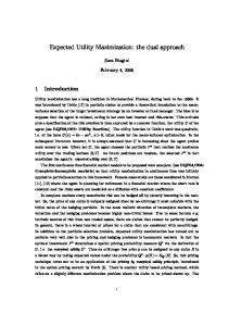
METHODS Case study of Sacramento & San Joaquin counties Our study area is delineated by the political boundaries of Sacramento and San Joaquin Counties (Fig. 1). This area contains two major cities, Sacramento and Stockton, and many other growing San Francisco Bay Area commuter towns and agricultural centers. The 6,26,730 ha area is comprised of 49.5% agricultural lands, 23% natural land cover (forests,
Kreitler et al. (2014), PeerJ, DOI 10.7717/peerj.690
4/19
Figure 1 Location of the study area. Study area of Sacramento and San Joaquin Counties (bold outlines), within California (inset), USA.
shrublands and grasslands), 21.5% developed area, and 5% wetland and open water. Between 1992 and 2008, 29,012 ha of agricultural lands were lost to urban development, primarily at the urban fringe. In Sacramento County, equal amounts of grassland and farmland were converted to urban development, while in San Joaquin County more than 75% of new urban land had been farmland. In addition to the economic and cultural impacts, loss of farmland in this region has implications for natural resource protection, as many of these lands would be considered multifunctional. Biodiversity is negatively affected by urban growth, and a large portion of the region with the potential for urban development occurs in low-lying areas with the possibility of catastrophic floods. Due to recent court rulings (Arreola v. County of Monterey; Paterno v. State of California), the State will ultimately be liable for flood damages (Fridirici, 2008; Duane, 2010) and potential economic damages to urban development are much greater than to agricultural land (Fridirici, 2008; Duane, 2010). Recent farmland losses in the region have prompted governmental and non-governmental action to preserve farmland from development. In San Joaquin County a farmland mitigation fee was established in an attempt to mitigate farmland losses. The Central Valley Farmland Trust, a non-profit land trust, was also established to facilitate the preservation of valuable agricultural land.
Kreitler et al. (2014), PeerJ, DOI 10.7717/peerj.690
5/19
Utility maximization in multifunctional agriculture conservation We used the utility maximization approach (Davis, Costello & Stoms, 2006; Machado et al., 2006) to allocate farmland conservation funds. The goal of this approach is to allocate farmland conservation funds to maximize the averted loss of multifunctional farmlands within the planning region through parcel acquisition. Without consideration of expected loss, funds may be ineffectively used to conserve land not likely to be converted (Newburn et al., 2005). We used the California Urban and Biodiversity Analysis model (CURBA, Landis & Reilly, 2002). to project urban growth in the region. Our approach also included the cost of conservation acquisition (section “Cost modeling”) to ensure resources were allocated cost-effectively. Each parcel received a utility score based on five criteria representing characteristics of multifunctional agriculture (sections “Combined benefit criteria”–“Sphere of influence”), and a utility function (section “Combined benefit criteria”). We then used two prioritization algorithms to select and compare sets of prioritized parcels for a given budget. Cost-effectiveness is calculated as a site’s utility score divided by the modeled acquisition cost to secure that utility from expected future loss. Combined benefit criteria We converted the five agricultural conservation criteria (agricultural viability, priority conservation areas, conservation buffers, flood liability, and sphere of influence, described below and in Machado et al. (2006) and Stoms, Kreitler & Davis (2011) for more detail), to marginal utility values before combining them through a weighted-linear combination (Malczewski, 1999). In this example the criteria are equally weighted, but user-defined weights could be applied to reflect varying social preferences for the function of agriculture. This takes the form: Bx = wj fj [Rj (x)] (1) j
where the combined utility (Bx ) is the sum of the products of each criterion-specific weight (wj ) and fj [Rj (x)], which is the marginal value of x according to utility function fj and representation level Rj . f j can take many functional forms, and this example we used a concave utility function as in previous studies (Davis, Costello & Stoms, 2006; Machado et al., 2006; Stoms, Kreitler & Davis, 2011). The representation level (Rj ) is the amount of the region specific non-threatened resource measured in criterion j . Agricultural viability We used a measure of agricultural viability to represent the potential for continued agricultural production on a given parcel. Agricultural viability was the product of estimated agricultural production capability and a measure of local condition (Machado et al., 2006). Production capability is a function of soil quality, climate, and water supply. Local condition was based on fragmentation of nearby lands and declines as urban land uses extend into agricultural lands (Bradshaw & Muller, 1998; Machado et al., 2006). To project agricultural viability in the future and model potential loss, we adjusted the
Kreitler et al. (2014), PeerJ, DOI 10.7717/peerj.690
6/19
production capability such that parcels projected to be developed had no production capability and local condition was updated based on the new urban frontier. Priority conservation areas We obtained data on priority conservation areas from a biodiversity conservation organization describing agricultural areas of interest for acquisition or conservation management. These zones integrate biodiversity conservation planning activities and serve as a proxy for a biodiversity conservation criterion. Within our study area there were eight separate areas ranging in size from 61 ha to 112,716 ha that were considered high conservation priority. Parcels were scored based on the amount of area falling within a priority conservation area that was also expected to be lost to development. While this criterion is not dynamic from the perspective of ensuring all species within the original conservation planning activities are covered, it is updated when conservation actions occur. Therefore, if a large portion of one priority conservation area is secured, the marginal value of the remaining area within that priority conservation area will be adjusted according to utility function, targets, and existing protected resources. Conservation buffers The conservation buffer criterion scored parcels based on the area contained within a parcel that fell within a one kilometer buffer around existing conservation lands. This criterion is based on the premise that areas immediately adjacent to reserves increase the effectiveness of the reserve by reducing the ecological contrast and associated edge effects between reserves and non-reserves and by providing additional habitat for wide ranging species, particularly for small reserves in working landscapes (Wiens, 2009). Flood liability The flood liability criterion prioritizes areas where farmland conservation would act as a flood risk reduction strategy by keeping urban development out of areas expected to flood (Kousky et al., 2013; Kousky & Walls, 2014). It is calculated by intersecting expected development and area within the hundred year floodplain. The CURBA model and an Army Corps of Engineers study (2002) were used to determine a parcel’s area in each zone. Parcels scoring high for this criterion have farmland within floodplains where land use conversion was expected.
Sphere of influence In California, local agency formation commissions (LAFCO) are required to delineate a sphere of influence surrounding incorporated areas that encourage orderly growth, preserve agricultural lands, and discourage urban sprawl (Fulton, 1999). The sphere of influence criterion scored parcels that are within a one kilometer buffer of spheres of influence around existing communities. In this manner, agricultural conservation was prioritized as a growth management tool to direct urbanization away from conservation resources (Stoms et al., 2009).
Kreitler et al. (2014), PeerJ, DOI 10.7717/peerj.690
7/19
Cost modeling Information on the cost of potential conservation actions plays a critical role in efficient conservation planning (Ando et al., 1998; Naidoo & Adamowicz, 2006; Naidoo & Ricketts, 2006; Newburn, Berck & Merenlender, 2006; Polasky, 2008; Stoms, Kreitler & Davis, 2011). In a typical conservation acquisition, resources are preserved through a conservation action, usually in the form of a purchase of property or development rights. With this action the resources are assumed to be protected from future loss. In some areas accurate data on land values are available, commonly through the local property tax assessor. In many areas the data are not accurate or available, so they must be modeled from observed transactions. Many studies rely on county or regionally averaged land values to determine the unit price of land (Polasky, Camm & Garber-Yonts, 2001; Davis, Costello & Stoms, 2006; Carwardine et al., 2008). Yet due to the common positive correlation between land cost and development threat (Ando et al., 1998), county averaged land values will likely underestimate the cost required to secure threatened resources, biasing the results of conservation plans. We therefore modeled the fine scale heterogeneity in potential acquisition costs at the parcel level to capture gradients of land value. We modeled land value at the parcel level using farmland property transactions acquired from the Dataquick real estate database service (www.dataquick.com). Using the hedonic pricing function of Rosen (1974) we estimated a predicted price per hectare within the two county study area. The potential value of urbanization of the parcel was capitalized in the market price. Variables from our model that explain per hectare variation in land value included parcel size, distance to urban areas, allowed uses, and presence within the one hundred year floodplain (p < 0.0045, r2 = 0.64).
Stochastic simulation Scheduling and land use change can impact the success of conservation actions (Armsworth et al., 2006; Wilson et al., 2006; Wilson et al., 2011), therefore, we simulated parcel availability as a stochastic process to determine the difference in accumulated utility when available sites were less than the full set (n = 31,020). A parcel availability matrix of 1,000 parcels by 4,000 simulations (40 time steps per 100 budget scenarios) was created with modeled probability of availability decreasing with increasing distance from urban centers, reflective of observed land use transitions in the region (Stewart & Duane, 2009; Duane, 2010). Selected (conserved) parcels were unavailable in subsequent time steps. Both solution procedures in the stochastic scenario drew from the same matrix of parcel availability at each step, therefore direct pairwise comparison of solution procedures is possible.
Solution procedures and comparison Using our dataset of multifunctional farmland utility we compared four scenarios. The IP and greedy heuristic solutions could select any parcel in the dataset, in any time period if the parcel had not already been prioritized for conservation action. We also performed both methods with a constraint of 1,000 available parcels in the land market at each time
Kreitler et al. (2014), PeerJ, DOI 10.7717/peerj.690
8/19
period (stochastic IP and stochastic greedy), to examine a situation more representative of what a conservation organization would face. All procedures follow the form: 1. Convert criteria scores to combined marginal values at each site (Eq. (1)). 2. Target sites to maximize the sum of B(x) subject to an annual budget (both IP and greedy). 3. Recalculate representation levels for each criterion (Rj ). 4. Recalculate marginal values at all unselected sites. 5. Continue steps 2–4 for a specified time period or total budget amount. 6. Calculate total utility of the selected set for comparison. Both solution procedures were written in the R statistical modeling environment (R Development Core Team, 2010). More detail on incorporating the IP solver into the utility maximization approach is included as pseudocode in Appendix S1. The IP formulation used R package lpSolve with the lpSolve program (Berkelaar, 2008), a free open source linear and mixed integer problem solver that uses the Simplex algorithm (Danzig, 1998). This solver was used, as opposed to commercial software, to demonstrate a completely open source software solution. The greedy heuristic sorted the cost effectiveness score in descending order and selected sites until the budget constraint was met each time period. We modeled cost effectiveness as a site’s marginal value divided by its modeled acquisition cost. To compare the similarity of selected sets we used the Jaccard similarity index (Jaccard, 1901), an index commonly used in ecology to describe community similarity between pairs of samples based on the presence or absence of species in each sample. The Jaccard similarity index is calculated as the intersection of the two sets, divided by their union and ranges from 0 to 1.
RESULTS Spatial heterogeneity of multifunctional agricultural lands The combined utility score, modeled parcel acquisition price, and cost-effectiveness results are illustrated in Fig. 2. The equally weighted combined criteria score (Fig. 2A) shows areas of high net benefit for multifunctional agricultural lands around the developed areas in the southern portion of the study area (near the cities of Lodi, Stockton, and Tracy (Fig. 1)). This is likely due to the presence of prime agricultural lands, flood risk, and strategic position between communities and development threat. In Fig. 2B, parcel acquisition prices were largely dependent on parcel size and distance from urban areas. Parcel size generally increases with increasing distance from urban areas, so acquisition prices largely increase as distance from urban increases, even though per acre price is generally highest near the urban edge and declines with increasing distance. Figure 2C shows the cost-effectiveness of each parcel as the ratio of combined utility divided by modeled acquisition costs. Even with the higher per-acre cost factored in, the areas around Lodi, east and west of Stockton, surrounding Tracy, and to the east of Manteca have high cost-effectiveness. The majority of cost-effective parcels are located within San Joaquin County, though parcels are selected in southern Sacramento County as well.
Kreitler et al. (2014), PeerJ, DOI 10.7717/peerj.690
9/19
Figure 2 Benefit, cost, and cost-effectiveness data. Heterogeneity of combined criteria benefits (A), modeled parcel acquisition costs (B), and cost-effectiveness of each parcel, calculated as benefits/costs (C).
Comparison of solution procedures The selected sites both in the IP and greedy solution at the $200 million budget are relatively clustered and compact due to the spatial characteristics of the criteria models (Fig. 3). The two methods select relatively similar sets (Jaccard similarity = 0.89). However, a major difference between the IP and greedy procedures is that the sites unique to the IP solution are more numerous and smaller, whereas fewer, larger sites are selected solely by the greedy solution method (Fig. 3). A comparison of the total accumulated utility by solution procedure is illustrated in Fig. 4. The IP and greedy solutions begin to diverge once $20 million is spent, with the difference between IP and greedy gradually increasing until the total budget is spent at $200 million. By the end of the budget the IP solution has accumulated 7% more utility than the greedy. Accumulated utility increases sharply from the beginning of the selection in both procedures, and then tapers as sites with lower marginal utilities are selected. When the potential sites are limited to those hypothetically available at each time interval (1,000 of the 31,020), the total accumulated utility ranges from 88% to 70% of the optimal IP solution for the stochastic IP and greedy solutions, respectively. The distributions of utility for the stochastic solutions overlap at the start but are significantly different at all intervals, (paired t-test, t = −3.077, p < 0.002), and then completely separate by the end of the scenario. The mean difference in utility between solution procedures by the end of the budget is 8% (ranging between 5 and 12%), with a mean pairwise Jaccard similarity of 0.86 (ranging between 0.82 and 0.91).
Kreitler et al. (2014), PeerJ, DOI 10.7717/peerj.690
10/19
Figure 3 Divergence and agreement between solutions. Comparison of the $200 million ($US) scenario results for a subset of the study area where a large number of parcels are prioritized by both the greedy and IP solution procedures.
DISCUSSION This study mapped five criteria describing elements of multifunctional agriculture to determine a hypothetical conservation resource allocation plan for agricultural land conservation. We compared solution procedures to determine the difference between an optimal integer programming approach and a greedy heuristic in a utility maximization problem. Stoms, Kreitler & Davis (2011) showed the importance of including benefit-losscost data in this study area; in this effort we demonstrate the improvement found through optimization methods, and determine the decline in total utility when site availability is a stochastic process. Our results show that the optimal solution and the greedy solutions were similar, but in each case, the IP formulation outperformed the greedy heuristic by up to 12%. We have described the solution of a knapsack or packing problem (Martello, Pisinger & Toth, 2000; Caccetta & Kulanoot, 2001), in a utility maximization approach (Davis, Costello & Stoms, 2006; Wilson et al., 2006; Moilanen, Wilson & Possingham, 2009), where the IP formulation found an incrementally more efficient solution given the budget constraint. This can be observed in Fig. 3 by comparing the selected sites unique to each solution method. The IP solution used numerous small, less expensive sites to maximize the utility, whereas the greedy solution was 7% less effective by simply selecting parcels in order of decreasing cost-effectiveness. Another noteworthy result is the proximity of the upper limit of the
Kreitler et al. (2014), PeerJ, DOI 10.7717/peerj.690
11/19
Figure 4 Comparison of solution procedures by total utility and cumulative cost. Accumulated utility by solution procedure for level of cumulative expenditure. In the stochastic simulations, the shaded areas represent the ranges of values for each solution procedure.
stochastic IP result to the greedy result at the $200 m level (Fig. 4). Even with reduced site availability, the IP solution approaches the full greedy solution that had access to all sites in the study area. This result may be partially due to the interchangeability of sites as well as the IP solver finding better solutions. The methods described here have potential implications for many natural resource management applications. The papers reviewed in Table 1 all use a similar mathematical formulation in which an objective function is maximized subject to a budget constraint. Most do not employ optimization methods and could likely be improved by adopting optimal solution procedures as illustrated here, and reviewed elsewhere (Rodrigues & Gaston, 2002; Williams, ReVelle & Levin, 2004; Haight, Snyder & Revelle, 2005). Furthermore, future studies could utilize the accessibility of lpSolve in the flexible R modeling environment without having to rely on proprietary commercial software. This study is unique in its combination of integer programming and a benefit or utility function approach. We are not aware of the use of IP or other search methods within utility maximization planning for multiple criteria. Wilson et al. (2006) used optimization methods with a benefit function, but for the singular objective of maximizing species persistence by scheduling ecoregional conservation actions through space and time. The use of multiple criteria allows a broader suite of potential applications in restoration planning or ecosystem service conservation planning, for example. Instead of a utility function, process based models (Ferrier & Drielsma, 2010) or ecosystem service production functions (Nelson et al., 2008; Nelson et al., 2009) could be included to convert landscape
Kreitler et al. (2014), PeerJ, DOI 10.7717/peerj.690
12/19
patterns into restoration benefits or ecosystem service values for conservation resource allocation schedules that are reflective of social preferences. Perhaps the largest drawback of using IP is the linear constraint on problem formulation. This “first stage suboptimality” (Moilanen, 2008) occurs when a complicated problem is simplified to fit into a linear formulation for which there is a tractable globally optimal solution. In our methods we take this approach by simplifying our criteria models. For example, our models calculate initial criteria values according to subsections “Agricultural viability”–“Flood liability” and incorporate distance and contiguity measures. These criteria scores are converted to marginal utility values per Eq. (1) and dynamically updated after each round of conservation actions, but the spatial operations are not, which leads to a more tractable problem for optimization. In this paper we have measured Moilanen’s (2008) “second stage suboptimality”, or the difference between the exact IP and heuristic solutions. However, for the reasons described above there may be larger true differences between linearly formulated exact IP solutions and heuristic solutions found using more complicated and realistic nonlinear model formulations, even if a less accurate heuristic algorithm is used to solve the problem. By contrast, when the results of this study are compared to Stoms, Kreitler & Davis (2011), which used the same data and similar methods to conduct a sensitivity analysis, the largest benefit to maximizing utility is found through using the cost-effectiveness of conservation actions, rather than by including threat estimates or using optimal solution methods. Similar studies have shown the degree of suboptimality from the absence of threat data or from the solution algorithm is of comparable magnitudes to those found here (Moilanen & Cabeza, 2007; Moilanen, 2008). All of the examples from Table 1 that use the utility maximization approach of Davis, Costello & Stoms (2006) have occurred in regions of California where variation in land value may be a principle factor influencing conservation opportunity. This is important to note when considering the findings, and how generalizable they may be. One of the unique features of this study is the fine scale at which the costs and benefits were calculated, and the spatial correlation of threats from urban development and land value. In regions with less heterogeneity in land value, results would likely be driven more by the benefit surfaces than in this example. Similarly, differences between solution methods would likely diminish as the planning unit scale increases and the decision space decreases to a fewer number of planning units to choose from. Further sensitivity analysis on the selection of land use change scenarios would be a last step in determining the robustness of results to the data inputs required by this planning framework. The merits and shortfalls of pursuing optimality in conservation planning have received considerable attention, usually with reference to minimum set or maximal covering reserve selection problems (ReVelle, Williams & Boland, 2002; Moilanen, 2008). The framework of utility maximization planning, however, is different due to site values that are typically a function of increasing representation with nominal target values, and the ability to incorporate multiple criteria measured in different units (Davis, Costello & Stoms, 2006; Moilanen, Wilson & Possingham, 2009). The utility or benefit function actually
Kreitler et al. (2014), PeerJ, DOI 10.7717/peerj.690
13/19
makes utility maximization problems less suitable for IP, though we have described a stepwise procedure to accommodate the numerical requirements of IP and the problem formulation of multicriteria utility maximization planning. The existing conservation planning program Zonation (Moilanen, 2007), with its predefined benefit functions, could be particularly useful for utility maximization problems. Further similarities between the utility maximization approach and Zonation include the ability to incorporate several important data inputs including benefit, threat, and cost data; an iterative heuristic similar to our greedy heuristic; and a built in routine to dynamically update all sites’ marginal values after conservation action. Continued research into the application of these methods and different software solutions is warranted due to the increasing opportunity for use in applied conservation and natural resource management problems in ecosystem services, restoration planning, or multifunctional agriculture conservation prioritization, in addition to biodiversity conservation.
ADDITIONAL INFORMATION AND DECLARATIONS Funding This project was supported by National Research Initiative Grant no. 2005-35401-15320 from the USDA Cooperative State Research, Education, and Extension Service Rural Development Program, and the USGS Land Change Science Program. The funders had no role in study design, data collection and analysis, decision to publish, or preparation of the manuscript.
Grant Disclosures The following grant information was disclosed by the authors: USDA Cooperative State Research, Education, and Extension Service Rural Development Program: 2005-35401-15320. USGS Land Change Science Program.
Competing Interests Jason Kreitler is an employee of the United States Geological Survey. David M. Stoms is an employee of the California Energy Commission.
Author Contributions • Jason Kreitler conceived and designed the experiments, performed the experiments, analyzed the data, contributed reagents/materials/analysis tools, wrote the paper, prepared figures and/or tables, reviewed drafts of the paper. • David M. Stoms and Frank W. Davis conceived and designed the experiments, contributed reagents/materials/analysis tools, wrote the paper, reviewed drafts of the paper.
Supplemental Information Supplemental information for this article can be found online at http://dx.doi.org/ 10.7717/peerj.690#supplemental-information.
Kreitler et al. (2014), PeerJ, DOI 10.7717/peerj.690
14/19
REFERENCES Ando A, Camm J, Polasky S, Solow A. 1998. Species distributions, land values, and efficient conservation. Science 279:2126–2128 DOI 10.1126/science.279.5359.2126. Armsworth PR, Daily GC, Kareiva P, Sanchirico JN. 2006. Land market feedbacks can undermine biodiversity conservation. Proceedings of the National Academy of Sciences of the United States of America 103:5403–5408 DOI 10.1073/pnas.0505278103. Arreola v. County of Monterey. 2002. Page 722. California 4th District Court of Appeal. Berkelaar M. 2008. lpSolve: interface to Lp solve v. 5.5 to solve linear/integer programs. Available at http://lpsolve.sourceforge.net/5.5/ (accessed January 2010). Bradshaw TK, Muller B. 1998. Impacts of rapid urban growth on farmland conversion: application of new regional land use policy models and geographical information systems. Rural Sociology 63(1):1–25 DOI 10.1111/j.1549-0831.1998.tb00662.x. Bryan BA. 2010. Development and application of a model for robust, cost-effective investment in natural capital and ecosystem services. Biological Conservation 143:1737–1750 DOI 10.1016/j.biocon.2010.04.022. Bryan BA, Raymond CM, Crossman ND, Macdonald DH. 2010. Targeting the management of ecosystem services based on social values: where, what, and how? Landscape and Urban Planning 97:111–122 DOI 10.1016/j.landurbplan.2010.05.002. Caccetta L, Kulanoot A. 2001. Computational aspects of hard Knapsack problems. Nonlinear Analysis-Theory Methods & Applications 47:5547–5558 DOI 10.1016/S0362-546X(01)00658-7. Carwardine J, Wilson KA, Watts M, Etter A, Klein CJ, Possingham HP. 2008. Avoiding costly conservation mistakes: the importance of defining actions and costs in spatial priority setting. PLoS ONE 3(7):e2586 DOI 10.1371/journal.pone.0002586. Chan KMA, Daily GC. 2008. The payoff of conservation investments in tropical countryside. Proceedings of the National Academy of Sciences of the United States of America 105:19342–19347 DOI 10.1073/pnas.0810522105. Chan KMA, Shaw MR, Cameron DR, Underwood EC, Daily GC. 2006. Conservation planning for ecosystem services. PLoS Biology 4:2138–2152. Church RL. 1974. A synthesis of a class of public facility location models. Baltimore: The Johns Hopkins University. Church RL, Stoms DM, Davis FW. 1996. Reserve selection as a maximal covering location problem. Biological Conservation 76:105–112 DOI 10.1016/0006-3207(95)00102-6. Costello C, Polasky S. 2004. Dynamic reserve site selection. Resource and Energy Economics 26:157–174 DOI 10.1016/j.reseneeco.2003.11.005. Crossman ND, Bryan BA. 2006. Systematic landscape restoration using integer programming. Biological Conservation 128:369–383 DOI 10.1016/j.biocon.2005.10.004. Crossman ND, Bryan BA. 2009. Identifying cost-effective hotspots for restoring natural capital and enhancing landscape multifunctionality. Ecological Economics 68:654–668 DOI 10.1016/j.ecolecon.2008.05.003. Crossman ND, Connor JD, Bryan BA, Summers DM, Ginnivan J. 2010. Reconfiguring an irrigation landscape to improve provision of ecosystem services. Ecological Economics 69:1031–1042 DOI 10.1016/j.ecolecon.2009.11.020. Csuti B, Polasky S, Williams PH, Pressey RL, Camm JD, Kershaw M, Kiester AR, Downs B, Hamilton R, Huso M, Sahr K. 1997. A comparison of reserve selection algorithms using data on terrestrial vertebrates in Oregon. Biological Conservation 80:83–97 DOI 10.1016/S0006-3207(96)00068-7.
Kreitler et al. (2014), PeerJ, DOI 10.7717/peerj.690
15/19
Danzig G. 1998. Linear programming and extensions. Princeton, NJ: Priceton University Press. Davis FW, Costello C, Stoms D. 2006. Efficient conservation in a utility-maximization framework. Ecology and Society 11(1):33 Available at http://www.ecologyandsociety.org/vol11/iss1/art33/. Davis FW, Stoms DM, Costello CJ, Machado EA, Metz J, Gerrard R, Andelman S, Regan H, Church RL. 2003. A framework for setting land conservation priorities using multi-criteria scoring and an optimal fund allocation strategy. Report to the Resources Agency of California Santa Barbara: National Center for Ecological Analysis and Synthesis. Duane TP. 2010. Increasing the public benefits of agricultural conservation easements: an illustration with the Central Valley Farmland Trust in the San Joaquin Valley. Journal of Environmental Planning and Management 53:925–945 DOI 10.1080/09640568.2010.495487. Ferrier S, Drielsma M. 2010. Synthesis of pattern and process in biodiversity conservation assessment: a flexible whole-landscape modelling framework. Diversity and Distributions 16:386–402 DOI 10.1111/j.1472-4642.2010.00657.x. Fischer DT, Church RL. 2005. The SITES reserve selection system: a critical review. Environmental Modeling & Assessment 10:215–228 DOI 10.1007/s10666-005-9005-7. Fridirici R. 2008. Floods and people: new residential development into flood-prone areas in San Joaquin County, California. Natural Hazards Review 9:158–168 DOI 10.1061/(ASCE)1527-6988(2008)9:3(158). Fulton W. 1999. Guide to California planning. Point Arena, CA: Solano Press. Haight RG, Snyder SA, Revelle CS. 2005. Metropolitan open-space protection with uncertain site availability. Conservation Biology 19:327–337 DOI 10.1111/j.1523-1739.2005.00151.x. Hajkowicz S, Perraud JM, Dawes W, DeRose R. 2005. The strategic landscape investment model: a tool for mapping optimal environmental expenditure. Environmental Modelling & Software 20:1251–1262 DOI 10.1016/j.envsoft.2004.08.009. Hannah L, Midgley G, Hughes G, Bomhard B. 2005. The view from the cape. Extinction risk, protected areas, and climate change. Bioscience 55:231–242 DOI 10.1641/0006-3568(2005)055[0231:TVFTCE]2.0.CO;2. ´ Jaccard P. 1901. Etude comparative de la distribution florale dans une portion des Alpes et des Jura. Bulletin del la Soci´et´e Vaudoise des Sciences Naturelles 37:547–579. Kousky C, Olmstead SM, Walls MA, Macauley M. 2013. Strategically placing green infrastructure: cost-effective land conservation in the floodplain. Environmental Science & Technology 47:3563–3570 DOI 10.1021/es303938c. Kousky C, Walls M. 2014. Floodplain conservation as a flood mitigation strategy: examining costs and benefits. Ecological Economics 104:119–128 DOI 10.1016/j.ecolecon.2014.05.001. Landis J, Reilly M. 2002. How will we grow: baseline projections of California’s urban footprint through the year 2100. Berkeley, California: Institute of Urban and Regional Development, University of California. Machado EA, Stoms DM, Davis FW, Kreitler J. 2006. Prioritizing farmland preservation cost-effectively for multiple objectives. Journal of Soil and Water Conservation 61:250–258. Malczewski J. 1999. GIS and multicriteria decision analysis. New York: J. Wiley & Sons. Margules CR, Pressey RL. 2000. Systematic conservation planning. Nature 405:243–253 DOI 10.1038/35012251. Martello S, Pisinger D, Toth P. 2000. New trends in exact algorithms for the 0–1 knapsack problem. European Journal of Operational Research 123:325–332 DOI 10.1016/S0377-2217(99)00260-X.
Kreitler et al. (2014), PeerJ, DOI 10.7717/peerj.690
16/19
McBride MF, Wilson KA, Burger J, Fang YC, Lulow M, Olson D, O’Connell M, Possingham HP. 2010. Mathematical problem definition for ecological restoration planning. Ecological Modelling 221:2243–2250 DOI 10.1016/j.ecolmodel.2010.04.012. Meir E, Andelman S, Possingham HP. 2004. Does conservation planning matter in a dynamic and uncertain world? Ecology Letters 7:615–622 DOI 10.1111/j.1461-0248.2004.00624.x. Moilanen A. 2007. Landscape Zonation, benefit functions and target-based planning: unifying reserve selection strategies. Biological Conservation 134:571–579 DOI 10.1016/j.biocon.2006.09.008. Moilanen A. 2008. Two paths to a suboptimal solution—once more about optimality in reserve selection. Biological Conservation 141:1919–1923 DOI 10.1016/j.biocon.2008.04.018. Moilanen A, Cabeza M. 2007. Accounting for habitat loss rates in sequential reserve selection: simple methods for large problems. Biological Conservation 136:470–482 DOI 10.1016/j.biocon.2006.12.019. Moilanen A, Wilson K, Possingham H (eds.) 2009. Spatial conservation prioritization: quantitative methods and computational toos. Oxford: Oxford University Press. Murdoch W, Polasky S, Wilson KA, Possingham HP, Kareiva P, Shaw R. 2007. Maximizing return on investment in conservation. Biological Conservation 139:375–388 DOI 10.1016/j.biocon.2007.07.011. Naidoo R, Adamowicz WL. 2006. Modeling opportunity costs of conservation in transitional landscapes. Conservation Biology 20:490–500 DOI 10.1111/j.1523-1739.2006.00304.x. Naidoo R, Ricketts TH. 2006. Mapping the economic costs and benefits of conservation. PLoS Biology 4:2153–2164 DOI 10.1371/journal.pbio.0040360. Nelson E, Mendoza G, Regetz J, Polasky S, Tallis H, Cameron DR, Chan KMA, Daily GC, Goldstein J, Kareiva PM, Lonsdorf E, Naidoo R, Ricketts TH, Shaw MR. 2009. Modeling multiple ecosystem services, biodiversity conservation, commodity production, and tradeoffs at landscape scales. Frontiers in Ecology and the Environment 7:4–11 DOI 10.1890/080023. Nelson E, Polasky S, Lewis DJ, Plantingall AJ, Lonsdorf E, White D, Bael D, Lawler JJ. 2008. Efficiency of incentives to jointly increase carbon sequestration and species conservation on a landscape. Proceedings of the National Academy of Sciences of the United States of America 105:9471–9476 DOI 10.1073/pnas.0706178105. Newburn DA, Berck P, Merenlender AM. 2006. Habitat and open space at risk of land-use conversion: targeting strategies for land conservation. American Journal of Agricultural Economics 88:28–42 DOI 10.1111/j.1467-8276.2006.00837.x. Newburn D, Reed S, Berck P, Merenlender A. 2005. Economics and land-use change in prioritizing private land conservation. Conservation Biology 19:1411–1420 DOI 10.1111/j.1523-1739.2005.00199.x. Onal H. 2004. First-best, second-best, and heuristic solutions in conservation reserve site selection. Biological Conservation 115:55–62 DOI 10.1016/S0006-3207(03)00093-4. Paterno v. State of California. 2004. Page 998. California 4th District Court of Appeal. Phillips SJ, Williams P, Midgley G, Archer A. 2008. Optimizing dispersal corridors for the cape proteaceae using network flow. Ecological Applications 18:1200–1211 DOI 10.1890/07-0507.1. Polasky S. 2008. Why conservation planning needs socioeconomic data. Proceedings of the National Academy of Sciences of the United States of America 105:6505–6506 DOI 10.1073/pnas.0802815105.
Kreitler et al. (2014), PeerJ, DOI 10.7717/peerj.690
17/19
Polasky S, Camm JD, Garber-Yonts B. 2001. Selecting biological reserves cost-effectively: an application to terrestrial vertebrate conservation in Oregon. Land Economics 77:68–78 DOI 10.2307/3146981. Possingham H, Andelman S. 2000. Mathematical methods of identifying representative reserve networks. In: Ferson S, Burgman M, eds. Quantitative methods for conservation biology. New York: Springer-Verlag, 291–305. Pressey RL, Cabeza M, Watts ME, Cowling RM, Wilson KA. 2007. Conservation planning in a changing world. Trends in Ecology & Evolution 22:583–592 DOI 10.1016/j.tree.2007.10.001. Pressey RL, Possingham HP, Margules CR. 1996. Optimality in reserve selection algorithms: When does it matter and how much? Biological Conservation 76:259–267 DOI 10.1016/0006-3207(95)00120-4. R Development Core Team. 2010. R: a language and environment for statistical computing. Vienna: R Foundation for Statistical Computing. Renting H, Rossing WAH, Groot JCJ, Van der Ploeg JD, Laurent C, Perraud D, Stobbelaar DJ, Van Ittersum MK. 2009. Exploring multifunctional agriculture. A review of conceptual approaches and prospects for an integrative transitional framework. Journal of Environmental Management 90:S112–S123 DOI 10.1016/j.jenvman.2008.11.014. ReVelle CS, Williams JC, Boland JJ. 2002. Counterpart models in facility location science and reserve selection science. Environmental Modeling & Assessment 7:71–80 DOI 10.1023/A:1015641514293. Rodrigues ASL, Gaston KJ. 2002. Optimisation in reserve selection procedures—why not? Biological Conservation 107:123–129 DOI 10.1016/S0006-3207(02)00042-3. Rosen S. 1974. Hedonic prices and implicit markets—product differentiation in pure competition. Journal of Political Economy 82:34–55 DOI 10.1086/260169. Stewart B, Duane TP. 2009. Easement exchanges for agricultural conservation: a case study under the Williamson Act in California. Landscape Journal 28:181–197 DOI 10.3368/lj.28.2.181. Stoms DM, Jantz PA, Davis FW, DeAngelo G. 2009. Strategic targeting of agricultural conservation easements as a growth management tool. Land Use Policy 26:1149–1161 DOI 10.1016/j.landusepol.2009.02.004. Stoms DM, Kreitler J, Davis FW. 2011. The power of information for targeting cost-effective conservation investments in multifunctional farmlands. Environmental Modelling & Software 26:8–17 DOI 10.1016/j.envsoft.2010.03.008. Thomson JR, Moilanen AJ, Vesk PA, Bennett AF, Mac Nally R. 2009. Where and when to revegetate: a quantitative method for scheduling landscape reconstruction. Ecological Applications 19:817–828 DOI 10.1890/08-0915.1. Underwood EC, Klausmeyer KR, Morrison SA, Bode M, Shaw MR. 2009. Evaluating conservation spending for species return: a retrospective analysis in California. Conservation Letters 2:130–137 DOI 10.1111/j.1755-263X.2008.00018.x. Underwood EC, Shaw MR, Wilson KA, Kareiva P, Klausmeyer KR, McBride MF, Bode M, Morrison SA, Hoekstra JM, Possingham HP. 2008. Protecting biodiversity when money matters: maximizing return on investment. PLoS ONE 3(1):e1515 DOI 10.1371/journal.pone.0001515. USACE. 2002. Interim Report: Sacramento and San Joaquin River Basins Comprehensive Study. Sacramento, CA: USACE. Vanderkam RPD, Wiersma YF, King DJ. 2007. Heuristic algorithms vs. linear programs for designing efficient conservation reserve networks: evaluation of solution optimality and processing time. Biological Conservation 137:349–358 DOI 10.1016/j.biocon.2007.02.018.
Kreitler et al. (2014), PeerJ, DOI 10.7717/peerj.690
18/19
Wainger LA, King DM, Mack RN, Price EW, Maslin T. 2010. Can the concept of ecosystem services be practically applied to improve natural resource management decisions? Ecological Economics 69:978–987 DOI 10.1016/j.ecolecon.2009.12.011. Wiens JA. 2009. Landscape ecology as a foundation for sustainable conservation. Landscape Ecology 24:1053–1065 DOI 10.1007/s10980-008-9284-x. Williams JC, ReVelle CS, Levin SA. 2004. Using mathematical optimization models to design nature reserves. Frontiers in Ecology and the Environment 2:98–105 DOI 10.1890/1540-9295(2004)002[0098:UMOMTD]2.0.CO;2. Wilson K, Cabeza M, Klein C. 2009. Fundamental concepts of spatial conservation prioritization. In: Moilanen A, Possingham H, Wilson K, eds. Spatial conservation prioritization: quantitative methods and computational tools. Oxford: Oxford University Press, 16–27. Wilson KA, Carwardine J, Possingham HP. 2009. Setting conservation priorities. Annals of the New York Academy of Sciences 1162:237–264 DOI 10.1111/j.1749-6632.2009.04149.x. Wilson KA, Lulow M, Burger J, Fang YC, Andersen C, Olson D, O’Connell M, McBride MF. 2011. Optimal restoration: accounting for space, time and uncertainty. Journal of Applied Ecology 48:715–725 DOI 10.1111/j.1365-2664.2011.01975.x. Wilson KA, McBride MF, Bode M, Possingham HP. 2006. Prioritizing global conservation efforts. Nature 440:337–340 DOI 10.1038/nature04366. Wilson KA, Underwood EC, Morrison SA, Klausmeyer KR, Murdoch WW, Reyers B, Wardell-Johnson G, Marquet PA, Rundel PW, McBride MF, Pressey RL, Bode M, Hoekstra JM, Andelman S, Looker M, Rondinini C, Kareiva P, Shaw MR, Possingham HP. 2007. Conserving biodiversity efficiently: what to do, where, and when. PLoS Biology 5:1850–1861 DOI 10.1371/journal.pbio.0050223. Wuenscher T, Engel S, Wunder S. 2008. Spatial targeting of payments for environmental services: a tool for boosting conservation benefits. Ecological Economics 65:822–833 DOI 10.1016/j.ecolecon.2007.11.014.
Kreitler et al. (2014), PeerJ, DOI 10.7717/peerj.690
19/19