OPTIMIZATION METHODS IN FRACTIONAL ORDER CONTROL OF ...

Proceedings of the 10th International Symposium on Mechatronics and its Applications (ISMA15), Sharjah, UAE, December 8-10, 2015

OPTIMIZATION METHODS IN FRACTIONAL ORDER CONTROL OF ELECTRIC DRIVES: A COMPARATIVE STUDY Serein Al-Ratrout1, Ashraf Saleem2, Hisham Soliman2 1

Department of Information Technology, Al-Zahra College for Women, Muscat, Oman Department of Electrical and Computer Engineering, Sultan Qaboos University, Muscat, Oman

2

[email protected],(asaleem)(hsoliman1)@squ.edu.om

ABSTRACT This paper presents a comparative study on the optimization methods in fractional PID controller design for induction motor. Choosing the best optimization algorithm for tuning fractional order controllers is crucial in order obtain best system response. In this study genetic algorithm, local search, nonlinear sequential quadratic programming, and particle swarm optimization algorithms are used to tune a fractional PI controller for induction motors. A model of a real motor is used to design and test the controllers. The resulted fractional controllers are approximated using refined Oustaloup’s recursive filter in order to be implemented using digital controllers. The controllers’ speed tracking performance is tested in simulation and a comparative analysis has been conducted. Keywords: Fractional PID, induction motors, optimization algorithm. 1.

INTRODUCTION

Fractional calculus has attracted many researchers and developers in the field of control system design [1-3]. It is claimed that fractional-order differential equations can describe real world systems more adequately [4] and therefore it is gaining more significance in designing controllers. With no doubt, Proportional-Integral-Derivative (PID) controllers are most popular controllers used in industry [5]. Recently, with the advances in fractional calculus, an extended version of the classical PID controllers known as Fractional Order PID (FOPID) was introduced [3]. Podlubny has proposed a generalized form of the FOPID controller as PIλDμ controller where λ and μ are the non-integer order of the integrator and differentiator terms respectively. In order to design such controllers, five parameters should be tuned for best performance. Therefore, many tuning techniques and algorithms for obtaining the FOPID controllers parameters have been investigated. In [6], a tuning method based on classical Zigler-Nichols (ZN) and Åström-Hägglund (AH) is introduced. The parameters kp and ki are obtained using ZN rules while the initial value of the kd is obtained using AH method. Two nonlinear equations are then obtained critical frequency and critical gain in order to achieve specified phase margin. The values of λ and μ are then obtained from these equations using an optimization toolbox of MATLAB. In [7], Particle Swarm Optimization (PSO) is used to tune FOPID controller for electromagnetic actuator (EMA) system

for aero fin control (AFC). The performance characteristics that are used for the controller optimization are rise time, peak time and percentage overshoot. The results show that PSO performs better than conventional tuning methods. In this paper, we are comparing different optimization methods that can be used to tune FOPID controllers. These optimization algorithms includes (1) Genetic Algorithm (GA), (2) Local Search Optimization (LSO), (3) Sequential Quadratic Programming (SQP), and (4) Particle Swarm Optimization (PSO). In order to show the efficiency of each optimization algorithm, a real induction motor model is used as a case study. The FOPID controller parameters are first optimized using the root mean square error as an objective function. The step response is then obtained and compared for all four methods using Fractional-order Modeling and Control (FOMCON) toolbox in MATLAB [8]. Finally, the FOPID controllers are converted to an approximated integer transfer function using refined Oustaloup filter and tested in Simulink for a multi-step input. The rest of the paper is organized as follows: section 2 introduces the induction motor model that will be used in this study. FOPID background is presented in section 3 while section 4 presents the application of four different optimization algorithms for tuning the FOPID controller. The realization of the FOPID is discussed in section 5 and the paper is concluded in section 6. 2.

INDUCTION MOTOR MODELING

The mathematical models of the induction motors presented in this section are based on work done in [9]. The electrical dynamic equations can be presented using vector model in a two-axis rotating frame as, (1) (2) (3) (4) Where    

978-1-4673-7797-3/15/$31.00 ©2015 IEEE ISMA15-1

(Vds, Vqs) and (Vdr, Vqs) are the stator and rotor voltages on the reference frame axis (d,q) (Ids, Iqs) and (Idr, Iqs) are the stator and rotor currents on the reference frame axis (d,q) (ds, qs) and (dr, qs) are the stator and rotor fluxes on the reference frame axis (d,q) Rs, Rr are the stator and rotor resistances

Proceedings of the 10th International Symposium on Mechatronics and its Applications (ISMA15), Sharjah, UAE, December 8-10, 2015



 are the stator and the rotor angular velocities

The mechanical rotational equation is, (5) Where J is the motor interia, T is the motor torque, b is the friction coefficient, and TL is the torque load. The motor torque is directly related to the current-flux. Equations 1 to 5 shows the inherent nonlinearity of the induction motor model and the difficult-to-measure parameters, therefore system identification is considered to obtain mathematical model. In this work, Auto-Regressive Moving-Average with eXogenous noise (ARMAX) models was used. These models are discrete-time linear parametric models and are formulated as polynomial functions [10]. The transfer function (between the output and input) can be obtained using

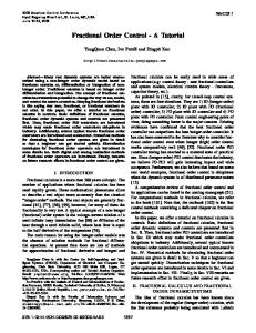
speed data measured by the dynamometer. A Sampling rate of 0.5 msec and output voltage level between 0 and 10 Volts were used. MATLAB/Simulink program was built using ARMAX blocks and RLS algorithm. The I/O data was then used to find ARMAX models for the plant. These models were then transformed to transfer functions with voltage as input and speed as output The motor was run in an open-loop environment under no-load and the measured speed results were recorded as shown in Figure 2. These input/output data were used to create a transfer function model of the motor using ARMAX model and RLS algorithm. The identified transfer function were converted from z-domain to s-domain using Tustin method. Following is the resulted function: G0 ( s) 

1840 s 3  7.361106 s 2 + 2.9451010 s + 1.1781014 s 4  8603s 3  4.187 107 s 2  7.0621010 s  7.1991011

(7)

This identified model was used to design and test the FOPID controller as explained in the following sections.

(6) Open loop speed response of an induction motor 1200

The Recursive Least Square (RLS) algorithm was used to update the model parameters vector.

1000

Figure 1 shows the experimental setup that was used to identify the induction motor under test. In this setup, the plant was composed of AC drive, a four-pole squirrel-cage three-phase induction motor, dynamometer, and a data acquisition system. The motor specifications were: stator voltage of 120/208 V, mechanical power of 200 W, nominal speed of 1685 rpm, nominal current of 1.14 A. The dynamometer specifications were: power rates of 240/415 V at 50 Hz, speed output signal resolution was 500 rpm per V, torque output signal resolution was 0.3 N.m per V, shaft encoder output of A/B-360 pulses and speed range of 290 to 3000 rpm, and external load control input sensitivity of 0.3 N.m/V.

Speed(rpm)

800

600

400

200

0

0

1

2

3

4

5 Time(s)

6

7

8

9

10

Figure 2. Open-loop motor step response Computer for data logging

3.

Data Acquisition unit

Processor and inverter Unit Induction Motor

Dynamometer

FRACTIONAL PID SPEED CONTROL

The most commonly used controllers in the industry are the PID type. Unlike the conventional integer order PID, a fractional order PID has been recently developed. The latter has more parameters to be tuned which provides more degrees of freedom and consequently better performance. The plant and the controller in feedback systems can be respectively modeled by the following transfer functions : (1) integer order (IO), fractional order (FO), (2) (FO), (IO), (3) both are (FO). The first case is considered in this study. Fractional order LTI systems are described by the fractional order differential equations in a general form written as : an Dn y(t )  ..  a1 D1 y(t )  ao y(t )  bm D m u(t )  ..  b1 D 1  bou(t ) (8)

Where α’s, β’s are D f (t )  s F ( s) fractions. By defining , a general the fractional order transfer function can be written as

Figure 1. Photo of the experimental setup The data acquisition system was composed of a PC and Data Acquisition Unit from LabVolt. The DAQ unit had 4 high voltage and high current inputs, 8 analog inputs with a range of ±10Vdc, 2 analog outputs, 3 digital inputs, 12 bits resolution, and maximum sampling rate of 600 kS/s. LabVolt 9063 Software Development Kit (SDK) was used to collect real

ISMA15-2

m

G( s) 

b s

i

 a s

i

i 0 n

i 0

i

i

(9)

Proceedings of the 10th International Symposium on Mechatronics and its Applications (ISMA15), Sharjah, UAE, December 8-10, 2015

k Gc ( s )  k p  I  k d s  s 4.

(10)

COMPARISON OF DIFFERENT OPTIMIZATION TECHNIQUES

In this section, four different optimization algorithms will be implemented to tune the FOPID for speed trajectory following of an induction motor. These optimization algorithms includes (1) Genetic Algorithm (GA), (2) Local Search Optimization (LSO), (3) Sequential Quadratic Programming (SQP), and (4) Particle Swarm Optimization (PSO). In order to guarantee fair comparison between the above algorithms and because it is required to trace a pre-defined speed trajectory, a fitness function based on root mean square error is used. This fitness function is as following

optimization, an iterative heuristic procedure for solving computationally hard problems is applied. The algorithm starts from some initial solution and search for a better solution in an appropriately defined neighborhood of the current solution. If a better solution is found, the current solution is replaced with the new solution and the algorithm repeats the same procedure from there. The algorithm repeatedly applies these steps until no better solution can be found in the neighborhood of the current solution. Figure 4 shows the flow chart of the adopted optimization algorithm that was used to solve the current problem. 1000

900

800

700

600

Speed(rpm)

In the case of FO-PID, the last equation reduces to

500

400

(11)

300

200

where RMSE is the fitness value, k is the order of the data, n is the total number of data, is reference speed and is the output speed. The PIDµ coefficient will be optimized so that the RMS error between the system output and the reference is minimum. 4.1. Optimization using Genetic Algorithm Referring to [11], the following GA operators and values are used in this work:  Coding: real number coding was chosen and therefore values of the PI coefficients are encoded with real numbers to form a single chromosome.  Population size: Population size influences the GA’s performance. After testing different population sizes, population size of N=20 was chosen.  Crossover: Arithmetic crossover operator is used with a probability value of 0.8.  Mutation: adaptive feasible operator is used.  Reproduction: Rank reproduction and elistic model operator are used. Elistic model is the transfer of four populations with best probability value to the next generation without any change. This should prevent the death of the most appropriate chromosomes. By applying the GA algorithm for tuning the FOPI, the following controller was obtained after 51 iterations with a fitness value of 0.0034, (12) This controller was tested on the motor model presented in section 2 using the FOMCON toolbox. Step response of the system is shown in Figure 3. It can be noticed that the rising time and settling time are 0.2s and 0.6s respectively. This can be considered as significant improvement compared to the open loop response. 4.2. Optimization using local search (LS) algorithm In order to find the coefficients kp, ki, kd, and , local search optimization algorithm can be adopted. In Local search

100

0

0

0.2

0.4

0.6

0.8

1 Time(s)

1.2

1.4

1.6

1.8

2

Figure 3. Step response of the system using GA optimized FOPI The resulted controller was obtained after 20 iterations, the fitness value was 0.0052, and the controller parameters were as following: (13) The step response of the system was obtained again using FOMCON toolbox as shown in Figure 5. The response of the system is better than the GA in terms of rising time and settling time. However, it is difficult in local search algorithms to select appropriate initial values and neighbors selection criterion. 4.3. Optimization Programming (SQP)

using

Sequential

Quadratic

One of the popular nonlinear programming methods is SQP. An overview of SQP can be found in [12] where the proposed method called interior point that can closely mimic Newton’s method for constrained optimization. At each major iteration an approximation is made of the Hessian of the Lagrangian function using a quasi-Newton updating method. This is then used to generate a QP sub-problem whose solution is used to form a search direction for a line search procedure. This method is already available in the optimization toolbox of MATLAB and can be executed using “fmincon” command. The interior point algorithm provided the best fitness value. A lower band of 0 has been used for the optimized parameters and the upper bounds was left open. The following controller was resulted from this algorithm with a fitness value of 0.04933 in 5 iterations, (14) It is noticed that >1 in this optimization. Figure 6 shows the step response of the optimized FOPI with the 0.1s rising time and almost no steady state error. This controller out performs the GA and LS controllers.

ISMA15-3

Proceedings of the 10th International Symposium on Mechatronics and its Applications (ISMA15), Sharjah, UAE, December 8-10, 2015

star t

(16)

Generate initial solution (kpi,kii,i)

(17)

Calculate initial fitness value (RMSEi)

: current velocity of agent I at iteration k : new velocity of agent I at iteration k, :adjustable cognitive acceleration constant, :adjustable social acceleration constant, :random number between 0 and 1, :current position of agent i at iteration k, :personal best of agent i, :global best of population.

Generate new neighbors (kpn,kin,n)

Rand1,2 Calculate new fitness value (RMSEn)

No

Pbesti gbest

RMSEn