such as modeling, design of a control law, implementation and validation. The self-tuning ..... (dominant poles method) of designing integral PID controllers [11].
Proceedings of 11th International Conference on Computer and Information Technology (ICCIT 2008) 25-27 December, 2008, Khulna, Bangladesh
Design of a Fractional-order Self-tuning Regulator using Optimization Algorithms Deepyaman Maiti, Mithun Chakraborty, Ayan Acharya, and Amit Konar Department of Electronics and Telecommunication Engineering, Jadavpur University, Kolkata, India system was caused mainly by the non-existence of simple mathematical tools for the description of such systems. Since major advances have been made in this area recently, it is possible to consider also the real order of the dynamical systems. Such models are more adequate for the description of dynamical systems with distributed parameters than integer-order models with concentrated parameters. It is necessary to understand the theory of fractional calculus in order to realize the significance of fractional order integration and derivation. Fractional calculus is the branch of calculus that generalizes the derivative or integral of a function to non-integer order, allowing calculations such as deriving a function to 1/2 order. For instance sα indicates derivation to the order α. Knowledge in the subject of fractional calculus is essential to design fractional order controllers. Of the several definitions of fractional derivatives, the Grunwald-Letnikov and Riemann-Liouville definitions are the most used [3]. These definitions are required for the realization of discrete control algorithms. The design of an STR can be divided into sub-tasks such as designing the modules for parameter estimation [4] and controller design [5]. For a chosen structure of a fractional order system, we have designed the ‘parameter identifier’ and ‘controller tuner’ blocks of Fig. 1. As a matter of fact, the controller we have considered is of a fractional order PID type, which differs from the usual integral order PID controller by the property that the orders of integration and derivation are positive real rather than restricted to only positive integers (conventionally unity). Fractional order PID controllers are much superior to their integer order counterparts, especially when controlling fractional order processes [6]. For designing the ‘parameter identifier’ block, we have made use of a stochastic optimization strategy from the family of evolutionary computation, namely particle swarm optimization (PSO) [7] – [8]. The ‘controller tuner’ block utilizes differential evolution (DE) [9] – [10]. Verification of the precision of our design is performed by operating the STR on a system with known parameters, and also by simulation. The robustness of our design is also displayed.
Abstract — The self-tuning regulators form an important sub-class of adaptive controllers. This paper introduces a novel scheme for designing a fractional order self-tuning regulator. Original designs for all the sub-modules of the self-tuning regulator are proposed. The particle swarm optimization algorithm is utilized for online identification of the parameters of the dynamic fractional order process while the subsequent tuning of the controller parameters is performed by differential evolution. Results show that the proposed self-tuning regulator is both precise and robust. Index Terms — Controller tuner, differential evolution, fractional order self-tuning regulator, parameter identifier, particle swarm optimization.
I. INTRODUCTION Development of a control system involves many tasks such as modeling, design of a control law, implementation and validation. The self-tuning regulator (STR) attempts to automate several of these tasks. This is illustrated in Fig. 1, which shows the block diagram of a process with an STR. It is assumed that the structure of the process is specified. Parameters of the process are estimated on-line by the block labeled ‘parameter identifier’. The block labeled ‘controller tuner’ contains computations that are required to perform the design of a controller with a specified method and a few design parameters that can be chosen externally. The design problem is called the underlying design problem for systems with known parameters. The block labeled ‘controller’ is an implementation of the controller whose parameters are obtained from the ‘controller tuner’ block [1]. In this paper we have presented a scheme for the design of a fractional order STR. This means that the physical process that needs to be controlled as well as the controller that will control it are both of fractional order. The real world objects or processes that we want to estimate are generally of fractional order [2]. A typical example of a non-integer (fractional) order system is the voltage-current relation of a semi-infinite lossy RC line or diffusion of heat into a semi-infinite solid, where heat flow q(t) is equal to the half-derivative of temperature T(t):
d 0 .5 T ( t ) dt 0 .5
= q ( t ).
So far, however, the usual practice when dealing with a fractional order process has been to use an integer order approximation. Disregarding the fractional order of the
1-4244-2136-7/08/$20.00 ©2008 IEEE
470
Fig. 1.
Block diagram of a self-tuning regulator
particle modifies its flying based on its own and companions’ experience at every iteration. The ith particle is denoted by Xi, where Xi = (xi1, xi2, …, xiD). Its best previous solution (pbest) is represented as Pi = (pi1, pi2, …, piD). Current velocity (position changing rate) is described by Vi, where Vi = (vi1, vi2, …, viD). Finally, the best solution achieved so far by the whole swarm (gbest) is represented as Pg = (pg1, pg2, …, pgD). The fitness function evaluates the performance of particles to determine whether the best fitting solution is achieved. The particles are manipulated according to the following equations:
II. STOCHASTIC OPTIMIZATION ALGORITHMS A. The Optimization Problem The optimization problem consists in determining the global optimum (in our case, minimum) of a continuous real-valued function of n independent variables x1, x2, x3, ⎛→⎞ …, xn, mathematically represented as f ⎜⎜ X ⎟⎟ , where ⎝ ⎠
vid (t + 1) = ωvid (t) + c1.ϕ1.(pid (t) − x id (t)) +
→
X = ( x 1 , x 2 , x 3 ,.....x n ) is called the parameter vector. Then the task of any optimization algorithm reduces to searching the n-dimensional hyperspace to locate a
c2 .ϕ 2 .(p gd (t) − x id (t)) x id ( t + 1) = x id ( t ) + v id ( t + 1) . (The equations are presented for the dth dimension of the position and velocity of the ith particle.) Here, c1 and c2 are two positive constants, called cognitive learning rate and social learning rate respectively, ϕ1 and ϕ2 are two random functions in the range [0,1], ω is the time-decreasing inertia factor which balances the global wide-range exploitation and the nearby exploration abilities of the swarm.
→
particular point with position-vector X D such that ⎛→ ⎞ ⎛→⎞ f ⎜⎜ X D ⎟⎟ is the global optimum of f ⎜⎜ X ⎟⎟ . ⎝ ⎠ ⎝ ⎠ B. Particle Swarm Optimization
The PSO algorithm [7] - [8] attempts to mimic the natural process of group communication of individual knowledge, which occurs when a social swarm elements flock, migrate, forage, etc. in order to achieve some optimum property such as configuration or location. The ‘swarm’ is initialized with a population of random solutions. Each particle in the swarm is a different possible set of the unknown parameters to be optimized. Representing a point in the solution space, each particle adjusts its flying toward a potential area according to its own flying experience and shares social information among particles. The particles swarm toward the best fitting solution encountered in previous iterations with the intent of encountering better solutions through the course of the process and eventually converging on a single minimum error solution. Let the swarm consist of N particles moving around in a D-dimensional search space. Each particle is initialized with a random position and a random velocity. Each
C. Differential Evolution
DE [9] - [10] belongs to the class of evolutionary algorithms guided by the principles of Darwinian Evolution and Natural Genetics where each time-varying parameter vector (candidate solution) in the population is called a chromosome and each time-step represents a generation. The first step of the algorithm, as usual, is: Initialization: This step is identical to the random initialization of position vectors in PSO. Each iteration consists of the following three steps: →
Mutation: For each chromosome X i ( t ) belonging to the →
current generation, three other chromosomes X p ( t ) , →
→
X q ( t ) and X r ( t ) are randomly selected from the same
471
generation (i, p, q and r are distinct); the scaled difference →
→
K p , Ti , Td are the proportional, integral and derivative
→
constants respectively, λ, δ are the orders of integration and derivation. We can have by simple block diagram algebra,
of X q ( t ) and X r ( t ) is added to X p ( t ) to generate a → → ⎛→ ⎞ V i ( t + 1) = X p ( t ) + F × ⎜⎜ X q ( t ) − X r ( t ) ⎟⎟ ⎝ ⎠ where F is a constant scalar in (0,1). We take F = 0.8.
donor
vector
→
K p + Ti s − λ + Td s δ C (s ) , = R (s ) K p + Ti s − λ + T d s δ + a 1 s α + a 2 s β + a 3
→
Recombination: A trial offspring vector T i ( t + 1) is
⎡ C (s ) ⎤ . ⇒ E ( s ) = R ( s ) − C ( s ) = R ( s ) ⎢1 − ⎥ R (s ) ⎦ ⎣
→
created for each current-generation parent vector X i ( t ) by first choosing a constant CR (0