Optimization of Control Parameters for Adaptive TrafficActuated Signal Control Will Recker Institute of Transportation Studies University of California, Irvine 4000 AIR Building Irvine, CA 92697-3600 USA Tel: +1-949-824-5642 Email:
[email protected] Xing Zheng Institute of Transportation Studies University of California, Irvine 4000 AIR Building Irvine, CA 92697-3600 USA Email:
[email protected] Lianyu Chu California Center for Innovative Transportation University of California, Berkeley 4000 AIR Building Irvine, CA 92697-3600 USA Tel: +1-949-824-1876 Email:
[email protected]
To be presented in ITS World Congress 2008, New York
-1-
ABSTRACT
This paper proposes a real-time adaptive control model for signalized intersections that decides optimal control parameters commonly found in modern actuated controllers, aiming to exploit the adaptive functionality of traffic-actuated control and to improve the performance of traffic-actuated signal system. This model incorporates a flow prediction process that estimates the future arrival rates and turning proportions at target intersection based on the available detector information and signal timing plan. Signal control parameters are optimized dynamically cycle-by-cycle to satisfy these estimated demands. The proposed adaptive control strategy is tested on a network consisting of thirty-eight actuated signals using microscopic simulation. Simulation results show the proposed adaptive model is able to improve the performance of the study network, especially under off-peak traffic conditions. Keywords: Adaptive signal control, optimization, microscopic simulation
INTRODUCTION At a signalized intersection, traffic signals typically operate in one of two control modes: pretimed and actuated (semi-actuated and full-actuated). In pre-timed control, all of the control parameters, such as cycle length, phase splits and phase sequence, are preset off-line based on an assumed deterministic demand level at different time periods of day. This control mode has only limited ability to accommodate the traffic fluctuations that are commonly found in reality. In actuated control, based on the vehicle actuations registered at detectors or other traffic sensors, cycle length, phase splits and even phase sequence can vary in response to current traffic demand. However, actuated controllers change these timings subject to a set of pre-defined, fixed parameters such as unit extension and maximum green, which do not “adapt to” current conditions. Real-time adaptive signal controls offer potential to satisfy non-linear and stochastic traffic demand patterns that tax the ability of actuated control. Existing adaptive controls that have been deployed, such as SCOOT (1) and SCATS (2, 3), which are considered “on-line” algorithms, adjust the timing parameters incrementally to accommodate changing traffic demands. This strategy is in fact to pick a “best” predetermined off-line timing plan with detector data to “match” current traffic. The major drawback of these systems is that they are not proactive, and hence cannot satisfy significant transients effectively. RHODESTM, a real-time traffic-adaptive signal control system developed at University of Arizona, uses a traffic flow arrivals algorithm--PREDICT (4)--to improve effectiveness when calculating online phase timings. In the PREDICT algorithm, detector information on approaches of every upstream intersections, together with the traffic state, and control plan for the upstream signals are used to predict future traffic volume. It assumes that all surrounding upstream intersections have fixed-time signalized planning, an assumption that is violated in virtually every modern system.
-2-
In none of these previous systems do the embedded traffic flow prediction models fully utilize available detector information and control features. Consequently, their applicability is confined only to particular factors, and thus restricted in achieving comprehensively good performance. And, although a number of theoretical issues involving, truly adaptive, systems have been explored and proposed (5, 6, 7, 8, 9, 10, and 11), their applicability to a functional model capable of addressing real-world situations has not been tested. For any signalized intersection, at least three kinds of information—vehicle actuated detector information, signal timing plan and current signal phase information—can be exploited to infer a relatively rich body of information that can be used in adapting the operation of a signal controller to current or expected conditions. The proposed adaptive control strategy developed in this paper incorporates a traffic flow prediction model that sufficiently utilizes all available information gleaned from signalized intersections to estimate the future arrival flows. Then optimal timing parameters are calculated based on the estimation for each signal phase in the study cycle. The optimized timing parameters are used as signal phase information for further estimations. This on-line, dynamically recursive computation process properly reflects the functionality of truly adaptive controllers. Particularly noteworthy here is that the adaptive control model proposed in this paper aims to provide an adaptive trafficactuated control strategy for off-peak periods, and not for peak-period conditions under which fixed-time or/and actuated signal coordination control is often employed quite effectively. This paper is organized as follows. The adaptive control model is described in detail in the next section. Then, the adaptive signal control model is tested within a microscopic simulation model, Paramics. Finally, conclusions are given.
METHODOLOGY Methodology Overview The proposed adaptive intersection control strategy incorporates a traffic flow prediction model that is an extension of Liu et al (12) to estimate approach volumes based on the outflows from upstream signalized intersection and forecasts turning movements at downstream intersection according to the turning fractions in previous cycles. Thus, the future flow rate associated with each phase at a downstream signal is decided by multiplying the estimated approach flow and corresponding turning proportion. Appropriate phase timing parameters are then computed in accordance with these estimated flow rates. In the model formulation, we restrict our control to only those parameters commonly found in modern actuated controllers: minimum green time, maximum green time and unit extension (gap time). Minimum green is computed based on the queue theory, determining an expected minimum green period required to dissipate the queue formed during red interval and the initial green period; maximum green is calculated according to the Webster’s function, accounting for any spillover from previous cycle. In determining gap time, we extend the approach taken by McNeil (5) to formulate a nonlinear optimization problem with objective minimizing total -3-
intersection control delay per cycle. Using LINDO--nonlinear program solver--we obtain optimal solutions, i.e. the gap times for all phases that minimize the control delay under gapout conditions. In any cycle in which gaps in traffic are less than this optimal gap time gapout control does not prevail and the corresponding phase will terminate by max-out control. These optimized timing parameters are used both for the upcoming cycle as well as provide phase information in further estimations. The optimization process is shown in Figure 1. Flow Prediction
Phase and Detector Information
Queue Theory Webster’s Function LINDO
Control Parameter Optimization
Signal Control
Figure 1 Optimization Process Components of a Signal Phase Generally in full-actuated control, phase split G consists of four portions. The first portion is the minimum green time Gmin, followed by one unit extension time. If a vehicle actuates the extension detector within the unit extension, the green period is extended by another unit extension time from the moment of actuation. This fashion repeats until the termination of green interval either by max-out control, in which green extension reaches maximum allowable green, or by gap-out control, in which no vehicle is detected by extension detector during a unit extension. The second portion is defined here as the waiting time Z, which is the green period from the end of minimum green to the beginning of the unit extension time which incurs gap out. The third part equals unit extension β. The last part of phase split is the pre-defined, fixed change and clearance time y+r. The rest period in the cycle is the red duration time R. (Figure 2) Rij
Giminj
Zij
βij
yi + ri
Rij+1
Figure 2 Phase Split (phase i in cycle j) Minimum green time Gmin and gap time β are two of the objectives in our adaptive control model and will be discussed in the following subsections. However, it is worthwhile to note here that Gmin is expected to be a variant green period that is long enough to clear vehicles queued at the stop line, and β is expected to be a particular gap time during which no vehicle actuates the extension detector, i.e. arriving vehicles during waiting time Z will not be obstructed by queuing vehicles and travel freely until gap out control materializes after the specific gap time β. -4-
The vehicle arrival pattern is assumed to be a Poisson process with average flow rate λ — strictly speaking, this assumption limits the application of the model to non-congested periods of operation. Vehicle headways then have a negative exponential distribution and the number of headways before the first one that is sufficiently large enough to invoke gap out has a geometric distribution. Then we have probability (at least on vehicle arrives in time β) = 1- e-λβ and probability (no vehicle arrives in time β) = e-λβ according to the negative exponential distribution, and probability (number of headways at which first headway larger than β occurs) = (1-e-λβ)n-1e-λβ with average value eλβ according to the geometric distribution. Therefore, approximately after eλβ headways, the green interval will terminate by gap-out. During these eλβ headways, eλβ -1 vehicles have passed the extension detector freely at flow rate λ, then the total green extension time Z + β is approximately (eλβ -1)/λ . So, the waiting time Z for phase i in cycle j is Zij =[exp(λijβij)– 1] / λij - βij
(1)
For ease of analysis, the displayed green interval, Gmin+Z+β, is usually converted to effective green ge; then the difference of phase split and effective green is the total lost time L (start-up lost time l1 and clearance lost time l2, assumed constant), while the difference of cycle length and effective green is the effective red re, which is equal to R+L. (Figure 3) When signal turns green, the first few vehicles will experience a start-up lost time l1, after which the queued vehicles, if any, will discharge at the saturation flow rate S (assumed constant) until the queue dissipates. This green period, during which vehicles cross the stop line at saturation flow rate, is defined as queue service time or saturated green period P. (Figure 4) giej-1
l2
Rij
giej
l1
l2
Figure 3 Effective Green and Effective Red Number Arrival Pattern (λij)
Discharge Pattern (Si)
riej = Rij + Li
Pij
Figure 4 Arrival and Discharge Pattern -5-
From Figure 4 and based on queue theory, the total number of vehicles departing at saturation flow during queue service time is equal to the sum of initial queue Q if any, plus arrived vehicles during effective red period and those during queue service time. Then we have Si × Pij = Qij + λij × (Rij + Li) + λij × Pij Therefore, Pij = [Qij + λij × (Rij + Li)] / (Si - λij )
(2)
It should be noted here that at the moment the queue service time expires, all queued vehicles have crossed the stop line, while it is highly possible that some following vehicles are already travelling in the road section between the stop line and the extension detector. As shown in Figure 5a for example, when queue service time expires, all queuing vehicles (in grey) have entered the intersection and the free vehicles (in white) that can enter intersection without slowing and stop, are approaching the stop line with the first one having a headway h to the stop line. Since the optimal gap time setting is expected to operate on all of the free vehicles that would traverse the intersection during green period (otherwise the calculated waiting time Z is biased), the waiting time Z is supposed to start before the end of queue service time P. Assuming that free vehicles, at least the first one, travel at a relatively constant speed from the extension detector to the stop line, we can get the situation U units of time backwards, as shown in Figure 5b. The first free vehicle is with headway h right behind the extension detector and this is the first headway on which the optimized gap time setting should operate. Note here that U is the original or the traditionally pre-set passage time based on the design speed and the set back detector’s placement. Further assuming that, when the green interval terminates, free vehicles that can use part of change and clearance interval as green extension still have U units of time to enter the intersection, we can compute the effective green and phase split as geij = Pij–Ui+Zij+βij+Ui=Pij+Zij+βij=[Qij+λij×(Rij+Li)]/(Si-λij)+[exp(λijβij)–1]/λij Gij = geij + Li = [Qij + λijRij + SiLi)] / (Si - λij ) + [exp(λijβij) – 1] / λij
h
Figure 5a when P expires
h
Figure 5b when Z begins -6-
(3) (4)
Estimating Arrival Flow In a network, the arrival flow at each leg of the downstream intersection is contributed by the corresponding phase outflows from upstream intersections, assuming no midblock exists on the links and no U-turn allowed at upstream intersections. Hence, the phase control strategy and phase timings of upstream signals are of great importance in determining the approach flow toward the downstream signal. In this paper, we introduce a flow prediction model that, first, utilizes the available phase information from upstream intersections to estimate the approach flow toward downstream intersections, and second, uses previous downstream signal phase timing to estimate the turning proportion. Referring to Figure 6 for example, two intersections are connected by a single link (right turn flow is ignored). The approach flow is the sum of outflows of phase 3 and 6 at upstream signalized intersection k and consists of inflows for phase 1 and 6 at downstream signalized intersection m. 1
2
3
4
5
6
7
8 m
k
Figure 6 Two-Intersection Network For upstream intersection k, the phase outflow is computed as the total vehicles served in the phase divided by the cycle length, then qikj = Nij / Ckj = [Si × Pij + λij × (Zij + βij)] / Ckj
(5)
Ckj = sum (G1kj + G2kj + G3kj + G4kj) or sum (G5kj + G6kj + G7kj + G8kj)
(6)
where
For downstream intersection m, referring to eq.(4), we get a nonlinear function of flow rate λij, which can be solved with many methods, such as Newton’s Algorithm: F(λij) = [Qij + λijRij + SiLi)] / (Si - λij ) + [exp(λijβij) – 1] / λij – Gij = 0
(7)
In this paper, a weighted moving average model is adopted to estimate the turning fractions TF, with different weights, 0.5, 0.3 and 0.2 for three previous turning proportions respectively. Then we have TFij = λij / (λij + λrj) ; ir = 16,25,38,47,61,52,83,74
(8)
TFij+1 = 0.5 × TFij + 0.3 × TFij-1 + 0.2 × TFij-2
(9)
Therefore, the arrival rate is equal to -7-
λij+1 = TFij+1 × qi+rj+1, λrj+1 = TFrj+1 × qi+rj+1 ; ir = 16,25,38,47,61,52,83,74
(10)
Determining Minimum Green Conventionally, minimum green is computed based on the number of vehicle actuations counted during the red period, which is a common method in volume density control type. This minimum green time, however, may not be sufficient to clear the queue formed at the stop line because, there is a chance that during the minimum green time, arriving vehicles will join the queue at the stop line causing a “sluggish” congested period and not completely enter the intersection when minimum green expires. Another fact that needs to be considered is that when the minimum green time ends, the gap time setting starts operation. Considering these two factors, we set the minimum green time with introducing the queue service time mentioned previously. Then we have Gminj+1 = l1 + Pij+1 - Ui = l1 + [Qij+1 + λij+1 × (Rij+1 + Li)] / (Si - λij+1 ) - Ui
(11)
Determining Maximum Green In determining maximum green, Webster’s equation Dij+1=[λij+1+Qij+1(3600/Cmax)]/Si is used to express the effective green factor. Cmax is the maximum allowable cycle length and is set to 120 seconds in this study. Maximum green setting is actually allocation of maximum allowable effective green time and usually consists of two computations: determine critical path and distribute green time. For both the left and right portions of the ring, we obtain the critical path and maximum effective green time as: Left: Critical Path Dm*j+1+Dn*j+1 = max (D1j+1+D2j+1, D5j+1+D6j+1); mn=12,56 Right: Critical Path Dr*j+1+Dk*j+1 = max (D3j+1+D4j+1, D7j+1+D8j+1); mn=34,78 Gleftj+1=[Cmax–(Lm*+Ln*+Lr*+Lk*)] (Dm*j+1+Dn*j+1)/( Dm*j+1+Dn*j+1)+( Dr*j+1+Dk*j+1) Grightj+1=[Cmax–(Lm*+Ln*+Lr*+Lk*)] (Dr*j+1+Dk*j+1)/(Dm*j+1+Dn*j+1)+(Dr*j+1+Dk*j+1)
(12) (13) (14) (15)
Then, maximum green is allocated to each phase on the critical path: Gm*j+1 = Gleftj+1× Dm*j+1/( Dm*j+1+ Dn*j+1) Gn*j+1 = Gleftj+1× Dn*j+1/( Dm*j+1+ Dn*j+1) Gr*j+1 = Grightj+1× Dr*j+1/( Dr*j+1+ Dk*j+1) Gk*j+1 = Grightj+1× Dk*j+1/( Dr*j+1+ Dk*j+1)
(16) (17) (18) (19)
For non-critical phase, the maximum green can be calculated using the same philosophy. Further, maximum green time Gmax is compared with actual green time G-L or ge to decide whether the phase terminates by gap out or max out. Then the initial queue can be determined as gap out: Qij+1 = 0; and max out: Qij+1 = max [0, Qij+ λij × (Rij + Gi) - (PijSi + λijZij)] (20) Determining Gap Time -8-
To decide optimal gap time settings, we formulate a nonlinear optimization problem with the objective function as minimizing the total intersection control delay per cycle. The delay expression is given by Darroch (1964), which is a generalization of the well-known Webster formulation: Wij+1 = Si ·λij+1[(Rij+1)2 + Rij+1 (2Qij+1/λij+1 + 1/Si + 1/(Si - λij+1))] / 2(Si - λij+1)
(21)
The term Rij+1 in eq.(21) can be expressed as the sum of other phases’ splits, based on the circular dependency relationship in dual-ring controller: R1j+1= G2j + G3j + G4j R2j+1= G1j+1 + G3j + G4j R3j+1= G1j+1 + G2j+1 + G4j R4j+1= G1j+1 + G2j+1 + G3j+1 R5j+1= G6j + G7j + G8j R6j+1= G5j+1 + G7j + G8j R7j+1= G5j+1 + G6j+1 + G8j R8j+1= G5j+1 + G6j+1 + G7j+1
(22)
Gij and Gij+1 can be derived from eq.(4), therefore, in matrix form we express Rij+1: Rj+1 = fi (Rj, λj, λj+1, Qj, Qj+1, βj, βj+1)
(23)
Substituting eq.(23) into eq.(21), we have Wj+1 = φi (Rj, λj, λj+1, Qj, Qj+1, βj, βj+1)
(24)
Then the optimization problem is formulated as: min ∑ Wij+1 subject to
i=1,2……7,8
G1j+1 + G2j+1 = G5j+1 + G6j+1 G3j+1 + G4j+1 = G7j+1 + G8j+1 G1j+1 + G2j+1 + G3j+1 + G4j+1 ≤ Cmax G5j+1 + G6j+1 + G7j+1 + G8j+1 ≤ Cmax βij+1 ≥ 0 The optimal gap time setting can be obtained by solving the objective function with LINDO, a nonlinear program solver. If no optimal solution is found for a certain phase, we set an arbitrary gap time for that phase, say 1/Si.
TESTING The adaptive signal control model is tested using a scalable, high-performance microscopic simulation package, Paramics (13). Paramics has been widely used in the testing of various algorithms and evaluation of various Intelligent Transportation Systems (ITS) strategies -9-
because of its powerful Application Programming Interfaces (API), through which users can access the core models to customize and extend many features of the underlying simulation model without having to deal with the underlying proprietary source codes. The proposed adaptive signal control model is developed as a Paramics plugin through API programming.
Figure 7 Test Network The test network is shown in Figure 7, which is the so-called “Irvine Triangle” network located in southern California. A previous study calibrated the simulation network for the morning peak period from 6 to 10 AM (14). The network includes a 6-mile section of freeway I-405, a 3-mile section of freeway I-5, a 3-mile section of freeway SR-133 and several adjacent surface streets, including two parallel streets of I-405 (i.e. Alton Parkway and Barranca Parkway), one parallel streets of I-5 (Irvine Center Drive), and three crossing streets of I-405 (i.e. Culver Drive, Jeffery Road, and Sand Canyon Avenue), and etc. The network has a total of 38 actuated signals, which are operated under actuated signal coordination during peak periods and under free-mode operation during off-peak periods. The performance of the adaptive signal control model is tested under three scenarios: (1) High demand scenario: The scenario corresponds to traffic condition in the morning peak period and its demands are obtained from the calibrated simulation model directly; (2) Medium demand scenario: its demand is equivalent to 75% of the high demand scenario; (3) Low demand scenario: its demand is equivalent to 50% of the high demand scenario. Four performance measures are used to evaluate the performance of the proposed adaptive signal control model, which is applied to all 38 signals: (1) Average Travel Time (ATT); (2) Average Vehicle Speed (AVS); (3) Vehicle Mileage Traveled (VMT); and (4) Vehicle Hours Traveled (VHT). Simulations are performed for each scenario for 4 hours and 15 minutes. The first 15 minutes of simulation are considered as the warm-up period for vehicles to fill in the network, and - 10 -
only the last four hours of the simulations are analyzed. Five simulation runs are conducted per scenario in order to generate statistically meaningful results. The results from the median run are used for analysis and comparison. Table 1, 2 and 3 show the performances of these three scenarios. It is found that the network under adaptive control performs better than the default actuated signal control in all three scenarios: drivers spend less time in the network, but travel more distance with improved traveling speed. It is also found that the adaptive control network performs best in scenario 2 (medium demand), probably both because the model was developed based on the assumption that vehicle arrivals are a Poisson process, and it is under precisely such conditions that gap settings control operation. On the other hand, high demand may incur large ratio of max-out controls; alternatively, low volume may result in large gap time setting. In both cases the effect of optimal gap time setting is not expected to be significant. Table 1 Performance under low demand scenario ATT (s) AVS (mph) VMT (miles) VHT (hours) Baseline 290.0 52.1 378535.85 7268.16 Adaptive control 268.6 56.3 382860.15 6799.97 Improvement (%) -7.38 8.06 1.14 -6.44 Table 2 Performance under medium demand scenario ATT (s) AVS (mph) VMT (miles) Baseline Adaptive control Improvement (%)
Baseline Adaptive control Improvement (%)
340.3 277.6 -18.42
45.2 52.6 16.38
557699.02 573416.69 2.82
VHT (hours) 12534.73 10514.17 -16.12
Table 3 Performance under high demand scenario ATT (s) AVS (mph) VMT (miles)
VHT (hours)
338.4 319.8 -5.50
17147.97 16134.61 -5.91
44.5 47.4 6.52
762398.74 763687.24 0.17
CONCLUSIONS This paper introduces an adaptive signal control model that can be applied to an existing actuated signal control system to improve the performance, particularly during off-peak periods. The model was tested using micro-simulation. It is found that model performance was best under traffic conditions of medium intensity, where the assumed Poisson arrival process underlying the model is expected to be valid. In the real world, however, traffic conditions may not be consistent with the assumed Poisson process, especially at closely spaced intersections where coordinated control strategy should be taken into account. Future effort will be made to seek a more sophisticated intersection control model that includes: (1) a more accurate flow prediction model that considers platoon - 11 -
and dispersion factors in estimating approach flow between linked signals; (2) optimization of control parameters for traffic flow under both high-volume and low-volume conditions.
REFERENCES (1) Robertson, D.I., and Bretherton, R.D. (1991) Optimizing Networks of Traffic Signals in Real Time-The SCOOT Method, IEEE Transactions on Vehicular Technology, Vol. 40, No. 1, pp. 11-15 (2) P. R. Lowrie (1992) SCATS: A Traffic Responsive Method of Controlling Urban Traffic Control, Roads and Traffic Authority (3) Sims, A. G. and Dobinson, K. W. (1979) SCATS – Sydney Coordinated Adaptive Traffic System Philosophy and Benefits, International Symposium on Traffic Control Systems, Vol. 2B. (4) Head, K.L. (1995) An Event-Based Short-Term Traffic Flow Prediction Model, Transportation Research Record 1510, pp.45-52. (5) McNeil, Donald R. (1968) A Solution to the Fixed-Cycle Traffic Light Problem for Compound Poisson Arrivals, Journal of Applied Probability, Vol. 5, No. 3, pp. 624-635. (6) Allsop, Richard E. (1971) Delay-minimizing Settings for Fixed-time Traffic Signals at a Single Road Junction, J. Inst. Maths Applies 8, pp.164-185. (7) Gazis, D., R. Herman and A. Maradudin (1960) The Problem of the Amber Signal Light in Traffic Flow, Operations Research, Vol.8, No.1, pp.112-132. (8) Improta, G. and G.E. Cantarella (1984) Control System Design for an Individual Signalized Junction, Transportation Research B, Vol.18B, No.2, pp. 147-167. (9) Lin, Wei-Hua and Wang C. (2004) An Enhanced 0–1 Mixed-Integer LP Formulation for Traffic Signal Control, IEEE Transactions On Intelligent Transportation Systems, Vol. 5 (4). (10) Liu, C., R. Herman and D. C. Gazis (1996) A Review of the Yellow Interval Dilemma, Transportation Research A, Vol.30, No.5, pp. 333-348. (11) Wong, C.K., S.C. Wong (2003) Lane-based optimization of signal timings for isolated junctions, Transportation Research Part B Vol.37, pp. 63–84 (12) Liu, Henry, Jian Sun and Will Recker (2005) Dynamic Date-Driven Short-Term Traffic Flow Prediction Model for Signalized Intersections, 85th Transportation Research Board Annual Meeting (13) Gordon D. B. Cameron1 and Gordon I. D. (1996) PARAMICS-Parallel microscopic simulation of road traffic, The Journal of Supercomputing, vol. 10 (1), pp 25-53. (14) Chu, L., Liu X., Recker, W. (2004) Using Microscopic Simulation to Evaluate Potential Intelligent Transportation System Strategies under Nonrecurrent Congestion, Transportation Research Record 1886, pp.76-84.
- 12 -