Optimization of Operating Parameters for Low NOx ...

Article pubs.acs.org/EF

Optimization of Operating Parameters for Low NOx Emission in HighTemperature Air Combustion Zhongbao Wei,† Xiaolu Li,† Lijun Xu,*,† and Cheng Tan† †

School of Instrument Science and Opto-Electronic Engineering, Beihang University, Beijing 100191, People’s Republic of China S Supporting Information *

ABSTRACT: This paper focuses on determining the effects of operating parameters on NOx emission and parameters optimization to reduce NOx emission for high-temperature air combustion furnaces. For this purpose, the Taguchi method, based on computational fluid dynamics (CFD) modeling, was implemented. Eight factors were considered, including the velocity of air injection (A), the velocity of fuel injection (B), the oxygen concentration in preheated air (C), the preheated air temperature (D), fuel temperature (E), the interaction between A and B, the interaction between A and C, and the interaction between A and D. An L27 (313) orthogonal array was employed to arrange the CFD modeling tests. By analysis of variance, the degrees of effect of the selected factors are determined, which are as follows, in descending order: E, B, C, A, D, AB, AC, and AD. The major factors are found to be A, B, C, and E, while the other factors are considered to be secondary factors. The optimal operating conditions are determined to be A = 120 m/s, B = 85 m/s, C = 18.5%, D = 1493 K, and E = 298 K. Under the optimal operating condition, the concentration of NOx emission decreases by 25.45%, compared with the original operating condition.

1. INTRODUCTION Fossil fuels play a dominant role in electricity industries worldwide. According to the statistics, fossil fuel still possesses almost 90% of the world’s primary energy source.1 Considering the reducing fossil resource and increasing energy demand, how to improve thermal efficiency has been an international concern. Obviously, thermal efficiency can be improved by increasing combustion temperature. However, increasing the combustion temperature inevitably results in more pollutant emission (for example, more NOx emission). NOx is a series of air pollutant formed by the oxidization of nitrogen during the combustion process, which is harmful to the human body and threatens the environment. NOx emission is responsible for the formation of photochemical smog, which contributes to problems of many human organs, such as heart, lungs, and eyes. NOx-caused photochemical smog can also reduce or even stop the growth of plants by reducing photosynthesis. In addition, NOx participates in some key chain reactions and exhausts the ozone, leading to depletion of the ozone layer in the upper atmosphere. Consequently, it is necessary to develop new technologies to reduce NOx emission and to make the combustion process more environmentally friendly.2 In order to deal with the contradiction between high thermal efficiency and low NOx emission, a new technology called hightemperature air combustion technology has been introduced, which controls the oxygen concentration with the support of a high-temperature oxidizer.3 In high-temperature air combustion technology, the preheated air is diluted with recycled hot combustion products to result in low oxygen concentration and high temperature. The highly diluted preheated air is mixed with fuel to form a more uniform combustion zone, which gives better efficiency and higher radiation flux. Moreover, the peak temperature is suppressed, which guarantees a much lower NOx emission compared with the conventional combustion.4−6 © 2012 American Chemical Society

Nabil Rafidi and Wlodzimierz Blasiak numerically investigated the difference between conventional combustion and hightemperature air combustion; the result just corresponded to the theoretical description given above.7 Consequently, hightemperature air combustion technology is a promising candidate to solve the contradiction between high thermal efficiency and low NOx emission and has been widely used in industrial equipment. Considering the fact that the combustion reaction is very sensitive to the reaction environment, the choices of operating parameters are crucial in the operation of high-temperature air combustion furnaces to reduce NOx emissions. Therefore, it is of great realistic significance to study the effects of various factors on NOx emission and further obtain the optimal operating condition for high-temperature air combustion furnace. Relative researches have been implemented to determine the effects of single factors on NOx emission in high-temperature air combustion furnace, such as the effects of fuel and oxygen concentration,8,9 preheated air temperature,10 shapes of burner nozzles,11 burner position, and firing mode.12 These researches explained the theoretical fundamental of combustion and provided a basis to analyze the combustion system. However, these researches were not enough to guide the practical work. First, the complex interaction effects among different single factors were not concerned. In the combustion system, the choice of one factor may influence the effects of other factors on the entire system, so that simply discussing the effects of a single factor is not justifiable. Second, these researches were not enough to quantitatively analyze the degrees of effect of various factors. For a specific problem, there always exist some major factors and secondary factors. When a Received: February 13, 2012 Revised: April 19, 2012 Published: April 19, 2012 2821

dx.doi.org/10.1021/ef300254m | Energy Fuels 2012, 26, 2821−2829

Energy & Fuels

Article

Figure 1. Geometry of the furnace and burner: the left part is the plane figure of the burner, and the right part is the three-dimensional geometry of the furnace drawn in a Cartesian coordinate system.

Taguchi method was employed in this paper to realize these purposes.

practical problem is analyzed, the major factors should be considered first and the secondary factors can be considered second or even be neglected. For the above two disadvantages, a further study is necessary to extend the traditional singlefactor analysis into engineering application. Therefore, there is still a gap in multifactor analysis and parameter optimization to reduce NOx emissions for high-temperature air combustion furnaces. Generally speaking, a factorial experiment is required to obtain the optimal operating conditions, because analysis of the high-temperature air combustion system is a multifactor problem. However, a factorial experiment is impracticable, especially when the number of considered factors is large. Considering this, Taguchi method is an appropriate method to overcome the difficulty brought by huge number of tests. The Taguchi method, which is a leading optimization technology reducing the experimental cost, enables us to minimize the variability around the target when bringing the performance value to the target value.13 The Taguchi method scientifically arranges and analyzes the multifactor problems, picks up the representative tests to reflect the overall situation, which is an efficient method to understand the degrees of effect of various factors and to optimize operating parameters for engineering systems. In recent years, the Taguchi method has been applied to solve such various engineering problems.14,15 Computational fluid dynamics (CFD) modeling technology is widely used in the analysis of combustion system to explore the basic numerical method and the characteristic of combustions.16,17 CFD modeling is an effective tool to understand the complex combustion process in the furnace, considering the high speed of computer calculation and difficulty of carrying out field experiments. Moreover, CFD modeling method provides researchers with a routine to realize the three-dimensional measurement, which cannot be realized by the traditional measurement methods. CFD modeling technology is based on the numerical solution of conservation equations for fundamental equations for scalar variables.18,19 By solving these equations, predictions of flow, thermal characteristics, and pollution formation inside the furnace can be obtained. In recent years, CFD modeling technology has been more and more popular in almost all of the fields that are related to hydrodynamics, such as heat transfer analysis20 and combustion process modeling.21,22 The objective of this study is to optimize operating parameters for the described high-temperature air combustion furnace to reduce NOx emission, and to determine the degrees of effect of the selected factors. A CFD-modeling-based

2. CFD MODELING The commercial CFD code Fluent 6.3 was employed to model the combustion process and NOx formation in the furnace. The mathematical models are based on the numerical solution of conservation equations for mass, momentum, energy, and transport equations for scalar variables. By solving these equations, the predictions of flow, thermal characteristics and pollutant formation inside the furnace can be obtained. 2.1. Furnace Description and Computational Domain. The research objective was a rectangle furnace with dimensions of 2 m (width) × 2 m (height) × 6.25 m (length). An air channel with a diameter of 0.124 m was equipped in the center of a side wall, through which the preheated air was supplied. Four fuel jets were located at 0.28 m from the air channel with the diameter of 0.01 m, through which the fuel gas was injected into the furnace. Only two fuel jets, distributed symmetrically along the x-direction, worked in this study. The burner was a 1:1 copy of an NFK burner that was operated at 0.58 MW. During the test, the temperature and gas compositions in the furnace were monitored. All the measurements were obtained by traversing the furnace in the horizontal plane of the two fuel jets. The geometry of the furnace and burner is shown in Figure 1. 2.2. Numerical Models. A renormalization group (RNG) k−ε turbulence model was employed, considering the significant amount of swirl during the combustion process of gas fuel. The combustion process is fast in the furnace, while the time required for the fuel and oxygen to enter into the reaction zone is relatively slow. Consequently, the rate of chemical reaction kinetics can be ignored, because the overall reaction rate is controlled by turbulence mixing.23 Based on the above analyses, the Eddy-Breakup (EBU) model was chosen to model the combustion process. More details of the EBU model can be found in the literature.24 A discrete ordinates (DO) radiation model was used to model the radiation. Not only does this model take the effects of absorption coefficient and scatting coefficient into account, but also it allows one to use a gray-band model to model the nongray radiation. The weighted sum of gray gases model was employed to compute the absorption coefficient. It is a compromise model between a simplified gray model and the model that considers the absorption coefficient in each band. The time scales for NOx reactions are larger than that for turbulent mixing process and hydrocarbons combustion. Therefore, the reactions involved in the NOx chemistry can 2822

dx.doi.org/10.1021/ef300254m | Energy Fuels 2012, 26, 2821−2829

Energy & Fuels

Article

be separated from the combustion process.25 NOx formation is decided by different mechanisms, including thermal NO, prompt NO, fuel NO, and N2O intermediate mechanisms. In high-temperature air combustion, thermal NO is an important route for NOx formation. The formation of thermal NO is determined by the following three extended Zeldovich mechanisms:

2.3. Boundary Conditions. The two fuel jets and the air channel were defined as velocity inlets. The velocity and temperature of fuel were 100 m/s and 298 K, respectively. The composition of fuel is listed as follows: φ(CH4) = 87.8%, φ(C2H4) = 4.6%, φ(C3H8) = 1.6%, φ(C4H10) = 0.5%, and φ(N2) = 5.5%. The velocity and temperature of air were 85 m/s and 1573 K, respectively. The composition of preheated air is listed as follows: φ(O2) = 19.5%, φ(N2) = 59.1%, φ(H2O) = 15%, φ(CO2) = 6.4%, and φ(NO) = 110 ppm. The combustion products and part of nonreacted air exhaust through the exit were treated as the pressure outlets. 2.4. Grids Generation and Grid Independence Test. As a control-volume-based technology, Fluent methodology divides the entire region into numbers of individual cells to produce the discrete algebraic equations that can be integrated numerically. Considering the geometrical symmetry of computational domain, one-quarter of the furnace was taken as the object to model. The Gambit 2.3 software package was employed to generate the computational grids for the computational domain. The furnace was divided into three parts in the flow direction. The front part and end part were 2 m (w) × 2 m (h) × 4 m (L) and 2 m (w) × 2 m (h) × 2 m (L), respectively, both of which were meshed with structured hexahedral grids, while the middle part was meshed by hybrid grids to make a connection. The grids were refined in near burner zones, near outlet zones and near wall zones, where the flow properties were critical. Generally speaking, increasing the grid number will improve the accuracy of modeling, but increases the calculating time at the same time. Therefore, to realize acceptable accuracy and fast speed, the total number of grids must be compromised at a proper level by conducting grid independence tests. Five different numbers of grids were investigated: 50 000, 110 000, 180 000, 320 000, and 400 000. When the critical physical quantities do not change with the increasing grid number, the grid system is considered to be independent. In this paper, the distribution of temperature and NOx concentration were monitored by using the radial line 0.73 m away from the fuel jets in the x-direction, which are shown in Figures 2 and 3, respectively. The modeling results show that the performance under a grid number of 400 000 has negligible difference with that of 320 000, on the distribution of both temperature and NO x concentration. Therefore, the grid number of 400 000 was

k1

O + N2 ⇄ NO + N k2

(R1)

k3

O2 + N ⇄ NO + O k4

(R2)

k5

N + OH ⇄ NO + H k6

(R3)

According to the mass action law of reaction, the reaction rate equation can be expressed as d[NO] = k1[O][N2] + k 3[O2 ][N] + k5[N][OH] dt − k 2[NO][N] − k4[O][NO] − k6[H][NO] (1)

where ki is the rate coefficient of the ith reaction (i = 1, 2, ..., 6) and t is the reaction time. Based on the hypothesis of steady state, the net rate of NO formation can be determined as follows: d[NO] = dt 1+

1 k 2[NO] k 3[O2 ] + k5[OH]

⎛ 2k 2 × ⎜2k1[O][N2] − 2 [O ] k ⎝ 3 2 + k5[OH] ⎞ × (k4[O][NO]) + k6[H][NO]⎟ ⎠

⎛ −C ⎞ ki = Ai T Bi exp⎜ i ⎟ ⎝ T ⎠

(2)

(3)

where T is the temperature of reaction. The reaction constants Ai, Bi and Ci are taken from Baulch et al.26 For the fuel gas, which contains no nitrogen, the fuel NO mechanism was ignored. Furthermore, relative investigations concluded that the N2O-intermediate mechanism was of outstanding significance during low peak temperature.27 As a result, it is necessary to employ the N2O-intermediate mechanism. Because of the above discussion, thermal NO, prompt NO, and N2O-intermediate mechanisms were involved in this paper. The second-order upwind scheme was applied for the space derivatives of advection terms in all transport equations. The SIMPLE algorithm was employed to handle the velocity− pressure coupling in the flow field equations. The residual for the energy equation was kept at 1 × 10−6 as a convergence criterion, while the residuals for the other equations were kept at 1 × 10−3. The mass-weighted-averages of temperature at the exit and the maximum temperature of the entire fluid were also monitored as another convergence criterion. Besides, when the mass and energy balance of the system were obtained by monitoring the mass flow rate and total heat transfer rate, the calculations were considered to be convergent.

Figure 2. Distribution of the temperature along the selected line. 2823

dx.doi.org/10.1021/ef300254m | Energy Fuels 2012, 26, 2821−2829

Energy & Fuels

Article

this paper, it is the concentration of NOx emission). As the SNR value gets higher, the quality of product improves. The objective of system optimization is to maximize the SNR values of the considered factors. The Taguchi method employs a special design method known as orthogonal arrays to arrange the experiments. The method significantly reduces the time required for an experimental investigation by selecting a small number of experiments to reflect the overall situation. The procedure of the Taguchi method can be generalized into four steps: identification of objectives, selection of factors and levels, selection of orthogonal array method, and analysis of the result. More details about the Taguchi method can be found in the relative literature.29−31 3.2. Selection of Factors and Levels. For the formulated problem, eight factorsincluding five single factors and three interaction effectswere considered, according to the fundamental theory of NOx formation. The five single factors included the velocity of air injection (A), the velocity of fuel injection (B), the oxygen concentration in preheated air (C), the preheated air temperature (D), and the fuel temperature (E). The three interaction effects included AB, AC, and AD. Three levels were set for each of the five single-factors based on the original operating condition. The selection of factors and levels is showed in Table 1.

Figure 3. Distribution of the NOx concentration along the selected line.

chosen for the following modeling. The three-dimensional grid geometry of the furnace is shown in Figure 4.

3. TAGUCHI-METHOD-BASED PARAMETER OPTIMIZATION 3.1. Fundamental of the Taguchi Method. After the CFD modeling method was determined, an experimental design was urgently needed to perform modeling tests. Factorial design is inefficient, especially when a good number of factors and levels are involved. The Taguchi method, which was developed by Genichi Taguchi, is an effective method to avoid the disadvantages of factory design. As for the evaluation criterion, the Taguchi method employs SNR (signal-to-noise ratio) to measure the performance variability of the selected factors when the noise factors are included. The variable S (signal) represents the mean, and the variable N (noise) stands for the standard deviation. The Taguchi method defines three different forms of mean square deviations, including “the nominal the better”, “the larger the better”, and “the smaller the better”. The objective of this paper is to minimize the concentration of NOx emission, which belongs to “the smaller the better” situation. The SNR value is calculated using the following equation:28 ⎛ 1 SNR = − 10 log⎜⎜ ⎝r

r

⎞

j=1

⎠

∑ yj 2 ⎟⎟

Table 1. Selected Factors and Levels factor

Level 1

Level 2

Level 3

A B C D E

85 m/s 80 m/s 18.5% 1498 K 298 K

105 m/s 100 m/s 19.5% 1598 K 398 K

125 m/s 120 m/s 20.5% 1698 K 498 K

3.3. Orthogonal Array. The present problem includes five single factors with three levels and three interaction effects. The number of degrees of freedom (DOF) adds up to 22. Considering this, the recommended orthogonal array table is L27 (313).32 Twenty-seven (27) modeling tests were implemented, according to the orthogonal array table, each of which was done twice to guarantee the reliability of CFD modeling. The number of modeling tests will be 2 × 35 = 486 by factorial experiment, while this number decreases to 54 by orthogonal array, indicating a significant improvement in efficiency. 3.4. Analysis of Variance. To understand the effects of various factors on the evaluation criterion, the analysis of variance must be employed to obtain the order of the degree of

(4)

where r is the number of repetitions done for an experimental combination, yj is the response variable of the j th repetition (in

Figure 4. Three-dimensional grid geometry. 2824

dx.doi.org/10.1021/ef300254m | Energy Fuels 2012, 26, 2821−2829

Energy & Fuels

Article

effect. The result is listed in a table, which contains columns “sum of square deviation (SS)”, “degree of freedom (DOF)”, “variance (V)”, “F value”, and “p value”. Of all the information provided in the table, the p-value serves as a criterion, defined as the probability of obtaining a test statistic at least as extreme as the one that was actually observed, assuming that the null hypothesis is true. If the p-value is smaller than the critical value (a = 0.01), the effect is considered statistically significant. In analysis of variance, the total effect is divided into two parts: the effect caused by the factors and the effect caused by the experimental error. Therefore, the error should be subtracted from the sum of squares expression and the remaining part is called the pure sum of squares (SS′), which can be calculated as follows: SS′Factor = SSFactor − VError × DOFFactor

(5)

where SSFactor ′ is the pure sum-of-square deviation of a specific factor, SSFactor the sum-of-square deviation of a specific factor, VError the variance of error, and DOFFactor the number of degrees of freedom of a specific factor. In this paper, the significance test was quantitatively analyzed by contribution rate (P), which can be calculated as follows: PFactor (%) =

SS′Factor × 100 SSTotal

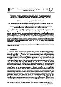
Figure 6. Comparison of predicted and measured NOx concentration distribution.

and stiff.33 Influenced by this, the modeled flowing state of fuel when it begins entering the furnace is different from that by measurement. Consequently, the modeled result deviates from the measured data unavoidably in the zone near to the jets. However, the present model accurately predicts the peak temperature, average temperature, and tendency of temperature change, all of which are related more directly to the NOx formation. Figure 6 shows the comparison of the predicted and measured distribution of NOx concentration along the radial line 0.15 m away from the fuel jets in the radial distance. Similar to the modeling result of temperature, the present model is unavoidably inaccurate in the zone near to the jets, because of the reasons explained above. However, the present model performs well in predicting the tendency of change in NOx concentration. Except for the zones near the jets, the modeling results correspond well with the measured data. Moreover, the modeled concentration of NOx emission is 144.6 ppm, with a relative error of 3.29% from the measured value of 140 ppm. Since the deviation is acceptable, the model presented in this paper can be validated to be used in the modeling of the NOx formation. 4.2. Modeling Results and SNR Calculation. The modeling results and the SNR values under the 27 different operating conditions are listed in Table 2. As can be seen from the modeling results, the minimum concentration of NOx emission is 130.8 ppm in case 16, while the maximum value reaches 808.9 ppm in case 24, almost five times larger than that in case 16. The concentration of NOx emission is sensitive to the operating condition, indicating that the selected factors have significant effects on NOx emission. 4.3. Analysis of Variance of Modeling Results. An analysis of variance of the SNR values was implemented to obtain the order of the degree of effect and to determine the major factors. The collected modeling data were analyzed using Minitab 16.0 software package, and the results are listed in Table 3. To better illustrate the degree of effect of selected factors to the concentration of NOx emission, the single contribution and cumulative contribution of the selected factors to the SNR value are shown in Figure 7. As can be seen from the result, A, B, C, and E are major factors that influence the concentration of NOx emission. The contributions of the four factors add up to 95.09% of all the considered factors. Moreover, the degrees of effect of the four

(6)

where SSTotal is the total sum of square deviation.

4. RESULTS AND DISCUSSION 4.1. Validation of CFD Model. To make a validation of the CFD model presented in this paper, the modeling result was

Figure 5. Comparison of predicted and measured temperature distribution.

compared with the experimental data from another published paper.33 Figure 5 shows the comparison of the predicted and measured temperature distribution along the radial line 0.15 m away from the fuel jets in the x-direction. The relative error of the predicted average temperature and peak temperature are 2.78% and 0.44%, respectively. It can be noticed that the present model fails to predict the position of peak temperature. This is because the modeling was implemented under steadystate conditions, which considers the fuel jets as straight and stiff. However, some nonstationary effects were involved in the practical combustion process for this furnace. As the reference states, the laser sheet visualization applied during the measurements suggests that the fuel jets are not strictly straight 2825

dx.doi.org/10.1021/ef300254m | Energy Fuels 2012, 26, 2821−2829

Energy & Fuels

Article

Table 2. Modeling Results and SNR Values Exp.

Result 1

Result 2

average

SNR

Exp.

Result 1

Result 2

average

SNR

1 2 3 4 5 6 7 8 9 10 11 12 13 14

156.4 375.5 727.8 246.7 139.2 238.4 142.4 201.8 132.3 559.2 360.4 582.1 205.8 423.3

150.2 366.1 712.3 238.4 148.6 242.6 142.6 211.6 134 542.7 369.2 605.6 209.3 404.3

153.3 370.8 720.1 242.6 143.9 240.5 142.5 206.7 133.2 551.0 364.8 593.9 207.6 413.8

−43.7 −51.4 −57.1 −47.7 −43.2 −47.6 −43.1 −46.3 −42.5 −54.8 −51.2 −55.5 −46.3 −52.3

15 16 17 18 19 20 21 22 23 24 25 26 27

239.9 131.2 248.1 424.6 371.7 635.9 485.4 148.5 405.8 795.2 332.4 160.8 395.3

246.5 130.4 261.3 448.9 365.2 664.3 508.6 145.3 390.4 822.6 338.8 166.7 381.5

243.2 130.8 254.7 436.8 368.5 650.1 497.0 146.9 398.1 808.9 335.6 163.8 388.4

−47.7 −42.3 −48.1 −52.8 −51.3 −56.3 −53.9 −43.3 −52.0 −58.2 −50.5 −44.3 −51.8

Table 3. Analysis of Variance of the SNR values parameter

SS

number of degrees of freedom, DOF

A B C D E AB AC AD errors total

90.66 167.07 107.39 5.99 227.13 5.82 5.80 4.07 2.86 616.80

2 2 2 2 2 4 4 4 4 26

a

V

F

p

45.33 83.54 53.70 3.00 113.57 1.46 1.45 1.02 0.72

63.32 116.69 75.00 4.18 158.63 2.03 2.02 1.42

0.001a 0.000a 0.001a 0.105 0.000a 0.254 0.256 0.371

The p-value was smaller than the significance level: a = 0.01.

Figure 8. Effect of each single factor to the SNR value.

Figure 7. Contribution of the selected factors to the SNR value.

major factors are determined, the descending order of which is as follows: E, B, C, and A. Factor D and interactions AB, AC, and AD contribute only 1.88% of all the considered factors; therefore, they are considered to be secondary factors. 4.4. Determination of the Optimal Operating Conditions. The major and secondary factors were determined via an analysis of variance, after which the optimal operating conditions were determined. The effect of each single factor on the SNR value is shown in Figure 8. As shown in Figure 8, the SNR value decreases by increasing the velocity of air injection. A higher velocity of air injection

Figure 9. Effect of the interaction effect between A and D (AD) to the SNR value.

results in a larger equivalence ratio and full combustion. As a result, more heat is generated, the temperature level is raised, and more NOx is formed. The SNR value increases as the velocity of fuel injection increases, because the equivalence ratio decreases, and the combustion tends to be incomplete. Under this situation, since 2826

dx.doi.org/10.1021/ef300254m | Energy Fuels 2012, 26, 2821−2829

Energy & Fuels

Article

Figure 10. Comparison of temperature field under the original and the optimal operating conditions: the temperature fields are shown in the horizontal plane of the two fuel jets. The temperature is presented in Kelvin units.

By increasing the air temperature, the SNR value decreases slightly at first and then the change is negligible, because a higher temperature of air injection leads to a higher temperature level in the furnace, and temperature is an important factor that influences the formation of thermal NO. Lastly, the SNR value dramatically decreases by increasing the fuel temperature, because the high fuel temperature decreases the activation energy of the combustion reaction and makes the reaction easy to conduct. However, the effect of fuel temperature obtained here is dissonant with the result of the existing reference.34 That is because the mass flow boundary condition is set for the injection in the reference. Increasing the fuel temperature accelerates the velocity of fuel injection, which shortens the residence time of the fuel in hightemperature region and finally results in low NOx emission. In contrast, the velocity boundary condition was set in this paper. The fuel temperature is considered alone, because the effect of the fuel temperature on the injection velocity is excluded, which discloses the effect of fuel temperature on NOx emission more definitively. To this point, the result in this paper is reasonable. The level with the largest SNR value for each factor has the best performance, as mentioned in section 3.1, and the combination of optimal levels indicates the optimal condition in the range of the experimental conditions. As for the four major factors, A1 (85 m/s) was the best choice of the velocity of air injection. B3 (120 m/s) was the best choice of the velocity of fuel injection. C1 (18.5%) was the best choice of the oxygen concentration in preheated air. E1 (298 K) was the best choice of the fuel temperature. When the level of D is selected, the effect of AD should be also considered, because the degree of effect of AD is similar to that of factor D. The effect of AD is shown in Figure 9. As a major factor, A should be maintained at Level 1. Under this constriction, the SNR values of A1D1, A1D2, and A1D3 are −45.88 dB, −50.05 dB, and −50.46 dB, respectively. The

Figure 11. Comparison of the distribution of NOx concentration under the original and the optimal operating conditions. Part of the horizontal plane of the two fuel jets is chosen to describe the NOx concentration distribution.

less heat is generated, the temperature is decreased and less NOx is formed. When increasing the oxygen concentration in preheated air, the SNR value becomes smaller. The increase of oxygen concentration in preheated air leads to an improvement of the average oxygen concentration in the furnace and results in more NOx generation, because oxygen plays a key role in the process of oxidizing combustion. 2827

dx.doi.org/10.1021/ef300254m | Energy Fuels 2012, 26, 2821−2829

Energy & Fuels

Article

Information. The L27 (313) orthogonal array employed in this paper is listed in Table 6 in the Supporting Information. The modeling experiments are implemented according to this table. After the modeling experiments are implemented, the collected data are treated by the Minitab 16.0 software package. The response of SNR value is listed in Table 7 in the Supporting Information; Figure 8 in the manuscript is drawn using the data in this table. This information is available free of charge via the Internet at http://pubs.acs.org/.

optimal selection should maintain the highest SNR value, indicating that D1 (1473 K) is the best choice for D. 4.5. Confirmatory Test under the Optimal Operating Conditions. Considering the fact that the optimal operating conditions were not included in the orthogonal array table, the final step of this paper was to confirm the discussion result by running another modeling test under the optimal operating conditions. When the confirmation modeling test was carried out, the grids generation method, numerical models, and boundary conditions were all maintained the same with the modeling tests done in the orthogonal array table. The comparison of temperature field under the original and the optimal operating conditions is shown in Figure 10. Under the optimal operating conditions, the temperature is lower than that under the original operating conditions. Moreover, the combustion zone is more uniform and no obvious hightemperature zone is found, compared to the original operating conditions. As can be seen from the confirmatory test result, the concentration of NOx emission is 107.8 ppm, which decreases by 25.45%, compared with the 144.6 ppm under the original operating conditions. The distribution of NOx concentration in the horizontal plane of the two fuel jets was obtained under both the original operating condition and the optimal operating condition, as shown in Figure 11. In this paper, only the part of the plane that is near the fuel jets was analyzed, because the remainder was uniform in NOx concentration. As can be seen, the NOx concentration under the optimal operating conditions was always less than that under the original operating conditions. From the above discussion, it can be concluded that the optimal operating condition obtained using the Taguchi method can reduce NOx emission efficiently.

■

Corresponding Author

*Tel.: +86 010 82317235. Fax: +86-010-82338319. E-mail: [email protected]. Notes

The authors declare no competing financial interest.

■

ACKNOWLEDGMENTS The authors gratefully acknowledge the financial support from the Project Supported by the National Natural Science Foundation of China (No. 60972087) and the Natural Science Foundation of Beijing, China (No. 3112018).

■

5. CONCLUSIONS A computational fluid dynamics (CFD)-modeling-based Taguchi method was implemented to optimize the operating parameters to reduce NOx emissions for high-temperature air combustion furnaces. By comparing the modeling result with the collected experimental data, the CFD model presented in this paper was validated for the purpose of investigating the combustion process and NOx formation in the furnace. The effects of selected parameters and interaction effects were systematically analyzed using the Taguchi method, through which 88.9% of the efforts that should be spent were saved. The result of analysis of variance indicates that the major factors are the velocity of air injection (A), the velocity of fuel injection (B), the oxygen concentration in preheated air (C), and the fuel temperature (E), while the secondary factors are the preheated air temperature (D), as well as the interactions between factors A and B (AB), factorrs A and C (AC), and factors A and D (AD). The final ranking of the degrees of effect, in descending order, is given as follows: E, B, C, A, D, AB, AC, and AD. The optimal operating conditions are found to be A1B3C1D1E1, which decreases the concentration of NOx emission by 25.45%, compared to the original operating conditions.

■

AUTHOR INFORMATION

NOMENCLATURE Ai, Bi, Ci = reaction constants of the i th reaction DOF = the degree of freedom F = value of F table j = index of repetitions done for an experimental combination ki = rate coefficient of forward reaction of the i th reaction P = percentage contribution r = number of repetitions done for an experimental combination SNR = signal-to-noise ratio SS = sum-of-square deviation t = reaction time T = reaction temperature V = variance yj = response variable of the j th repetition

Abbreviations

■

CFD = computational fluid dynamics EBU = eddy breakup DO = discrete ordinates

REFERENCES

(1) Edge, P. J.; Heggs, P. J.; Pourkashanian, M.; Stephenson, P. L.; Williams, A. Fuel 2011, DOI: 10.1016/fuel.2011.05.005. (2) Jarquin-López, G.; Polupan, G.; Toledo-Velázquez, M.; LugoLeyte, R. Appl. Therm. Eng. 2009, 29, 1614−1621. (3) Pan, L.; Ji, H.; Cheng, S.; Wu, C.; Yong, H. Appl. Therm. Eng. 2009, 29, 3426−3430. (4) He, R.; Suda, T.; Takafuji, M.; Hirata, T.; Sato, J. Fuel 2004, 83, 1133−1141. (5) Khoshhala, A.; Rahimi, M.; Alsairafi, A. A. Int. Commun. Heat Mass Transfer 2011, 38, 1421−1427. (6) Parente, A.; Galletti, C.; Tognotti, L. Int. J. Hydrogen Energy 2008, 33, 7553−7564. (7) Rafidi, N.; Blasiak, W. Appl. Therm. Eng. 2006, 26, 2027−2034. (8) Mohamed, H.; Bentîcha, H.; Mohamed, S. Combust. Sci. Technol. 2009, 181, 1078−1091. (9) Cao, Z.; Zhu, T.; Jin, C. 2010 International Conference on Mechanic Automation and Control Engineering (MACE), Wuhan, China, June 26−28, 201040104014

ASSOCIATED CONTENT

* Supporting Information S

Some other Supporting Information is provided here. The comparison between experimental data and modeling results is shown in a figure in the article. To support it, the data used in the figure are listed in Tables 4 and 5 in the Supporting 2828

dx.doi.org/10.1021/ef300254m | Energy Fuels 2012, 26, 2821−2829

Energy & Fuels

Article

(10) Khoshhal, A.; Rahimi, M.; Shabanian, S. R.; Alsairafi, A. A. Proc. World Acad. Sci., Eng. Technol. 2010, 62, 569−574. (11) Zheng, W.; Zhu, S.; Zhu, T. Power Eng. 2007, 27, 287−291. (12) Danon, B.; Cho, E. S.; de Jong, W.; Roekaerts, D. J. E. M. Appl. Therm. Eng. 2011, 31, 3000−3008. (13) Lang, Y.; Malacina, A.; Biegler, L. T.; Munteanu, S.; Madsen, J. I.; Zitney, S. E. Energy Fuels 2009, 23, 1695−1706. (14) Mahamuni, N. N.; Adewuyi, Y. G. Energy Fuels 2010, 24, 2120− 2126. (15) Surisetty, V. R.; Dalai, A. K.; Kozinski, J. Energy Fuels 2010, 24, 4130−4137. (16) Andersen, J.; Rasmussen, C. L.; Giselsson, T.; Glarborg, P. Energy Fuels 2009, 23, 1379−1389. (17) Zhou, H.; Mo, G.; Si, D.; Cen, K. Energy Fuels 2011, 25, 2004− 2012. (18) Zhou, H.; Mo, G.; Zhao, J.; Cen, K. Fuel 2011, 90, 1584−1590. (19) Wei, Q. S.; Lu, G.; Liu, J.; Shi, Y. S.; Dong, W. C.; Huang, S. H. Comput. Electron. Agr. 2008, 63, 294−303. (20) Lu, G.; Wei, Q. S.; Liu, J.; Shi, Y. S.; Dong, W. C. In 7th World Congress on Computers in Agriculture and Natural Resources Confernce Proceedings, Reno, NV, 2009; pp 170−177. (21) Zhou, H.; Mo, G.; Cen, K. Energy Fuels 2010, 24, 6294−6300. (22) Rahimi, M.; Khoshhal, A.; Shariati, S. M. Appl. Therm. Eng. 2006, 26, 2192−2200. (23) Spalding, B., D. Symp. (Int.) Combust. 1971, 13, 649−657. (24) Xue, H.; Ho, J. C.; Cheng, Y. M. Fire Saf. J. 2001, 36, 37−54. (25) Yang, W.; Blasiak, W. Fuel Process. Technol. 2005, 86, 943−957. (26) Baulch, D. L.; Drysdall, D. D.; Horne, D. G. Evaluated Kinetic Data for High Temperature Reactions; Butterworth: London, 1973. (27) Khoshhal, A.; Rahimi, M.; Alsairfi, A. A. Numer. Heat Transfer, Part A 2011, 59 (8), 633−651. (28) Kackar, N, R. J. Quality Technol. 1985, 17, 176−188. (29) Taguchi, G.; Quality Resources: New York, 1987. (30) Ross, P. J. Taguchi Techniques for Quality Engineering; McGraw− Hill: New York, 1988. (31) Yakut, K.; Sahin, B.; Celik, C.; Alemdaroglu, N.; Kurnuc, A. Appl. Energy 2005, 80, 77−95. (32) Barrett, J. D. In Taguchi’s Quality Engineering Handbook; Wiley: New York, 2007. (33) Mancini, M.; Weber, R.; Bollettini, U. Proc. Combust. Inst. 2002, 29, 1155−1163. (34) Yang, W.; Blasiak, W. Energy Fuels 2004, 18, 1329−1335.

2829

dx.doi.org/10.1021/ef300254m | Energy Fuels 2012, 26, 2821−2829