Preprints of the 19th World Congress The International Federation of Automatic Control Cape Town, South Africa. August 24-29, 2014
Optimization of Robotic Arm Trajectory Using Genetic Algorithm Stanislav Števo. Ivan Sekaj. Martin Dekan.
Institute of Control and Industrial Informatics Faculty of Electrical Engineering and Information Technology Slovak University of Technology, Ilkovičova 3, 812 19 Bratislava, Slovak Republic (e-mail:
[email protected],
[email protected],
[email protected]) Abstract: The paper presents a genetic algorithm - based design approach of the robotic arm trajectory control with the optimization of various criterions. The described methodology is based on the inverse kinematics problem and it additionally considers the minimization of the operating-time, and/or the minimization of energy consumption as well as the minimization of the sum of all rotation changes during the operation cycle. Each criterion evaluation includes the computationally demanding simulation of the arm movement. The proposed approach was verified and all the proposed criterions have been compared on the trajectory optimization of the industrial robot ABB IRB 6400FHD, which has six degrees of freedom. Keywords: Robotic arm trajectory, genetic algorithm, inverse kinematics problem, energy consumption minimization, operating time minimization, joint rotation minimization.
1. INTRODUCTION The optimisation of the robotic arm trajectory is a frequent design problem. Because of the complexity of this task in the past, many of the proposed approaches entailed only a suboptimal solution. Due to that reason, previously, several authors have used evolutionary algorithms. Rana and Zalzala (1997) applied EA to the collision-free path planning of the robotic arm. In Garg & Kumar (2002), the formulation and application of Genetic Algorithm and Simulated Annealing for the determination of an optimal trajectory of a multiple robotic configuration is presented. In Park et al. (1999) a method for optimal trajectory control using the Evolution Strategy is proposed. In the first step, the optimal trajectory based on the cubic polynomials under certain physical constraints is determined. In the second step, the fuzzy controller is optimized to precisely track the determined trajectory. Davidor (1991) uses Genetic Algorithms with regards to the trajectory generation by searching the inverse kinematics solutions to pre-defined paths of end-effectors. In Juang (2004) a multi-manipulator collision avoidance using Genetic Algorithms is presented, the safety distance between objects is affected by the repulsive force gain and real-time manipulator collision avoidance control has been achieved. Multi-objective Genetic Algorithm for generating manipulator trajectories considering obstacle avoidance is proposed in Pires (2004). The results are presented for robots with two and three degrees of freedom (DOF), considering two and five optimization objectives. An overview of using evolutionary algorithms in controller design and robotics can be found in Sekaj (2011). In the presented approach, the robotic arm trajectory design is based on inverse kinematics problem solving (IKP) with connection to further optimizations of selected criterions. The inverse kinematics problem of the robot – the dependency
Copyright © 2014 IFAC
between the joint variables and the coordinates of the end effector (or the end point of the arm) represents a complex problem with infinite number of possible solutions. The more DOF the robot has the more complex the calculation of the IKP is. An additional consideration of other optimization criterions into the IKP becomes a very difficult task, almost insolvable using conventional methods e.g. Garg & Kumar (2002), Juang (2004), Vigrala et al. (2013). We propose the solving of the IKP using additional criterions, which make the problem solvable with a powerful optimisation approach the Genetic Algorithm (GA). Three additional optimisation criterions (together with the positioning accuracy) are considered. These are the minimisation of energy consumption, minimisation of operation time as well as the criterion of minimal total angular changes of the robotic arm. 2. INVERSE KINEMATICS PROBLEM A robot with n degrees of freedom (Fig.1) has the joint rotation angles α1, α2, ..., αn and performs N operations in points P1 to PN defined in a clockwise cartesian coordinate system Pi[xi;yi;zi]. Each operating point (end effector of the manipulator) is characterized by n-angles of the joint rotation Pi[xi;yi;zi] f(α1i, α2i,...,αni);i {1,2,3,...,N}.
(1)
According to (1), the aim of the inverse kinematics task for the execution of a single robot cycle is the search for a sequence of N vectors of angles, which characterize the desired operating points. In general, using conventional design methods under consideration of additional criterions, it is not possible to solve the inverse kinematic task for a robotic arm with n degrees of freedom e.g. Pac et al. (2013), Vigala et al. (2013). To solve this problem it is possible to use other approaches as evolutionary algorithms. Because the
1748
19th IFAC World Congress Cape Town, South Africa. August 24-29, 2014
number of search parameters in such formulation of the task is constant, the Genetic Algorithm can be used. Each potential solution of the problem represents a vector of values S={α11, α21,..., αn1, ... , α1N, α2N,..., αnN},
(2)
Each potential solution (individual) represents the rotation of all robotic joints, which move in terms of the end effector between points P1to PN. The range of values for each parameter αj,i is from the interval min , max , which is the rotation range of each particular arm joint. The optimal solution is such a vector S*, which minimises the selected criterion.
The rotations of arms are forced by motors with rated outputs of EP1, EP2 to EPN. Energy consumed between two operational points counts as the energy consumed by motors during transition from one operating point to another. Energy consumed between two working points (p2p - point to point) Pa and Pb is then determined as ∑[(
1. 2. 3. 4.
5. 6. 7.
initialization of the population (set of individuals), fitness function (criterion) calculation of each individual of the population, if termination conditions are met, then finish (in our case - predefined number of generations), else continue in step 4, parent selection (more fit individuals have higher probability to be selected, in our case the stochastic universal sampling was used, 70% of individuals of the population were selected), modification of parents by crossover and mutation = children, completion of the new population (children + selected unchanged individuals), continue in step 2.
An individual is a string containing parameters of the optimized object. In our case, the individual is in the form (2). Mutation is an operation, where a parent individual is randomly changed (mutation rate was 0.1). Crossover is an operation, where properties of two parent individuals are randomly combined to produce a child (crossover rate used was 0.7). The fitness function evaluation contains the calculation (or a simulation) of the robot movement and the cost function evaluation. The cost function in our case contains at least two particular criterions. The population size used in our case was set as quadruple of the gene number.
Energy needed for the entire trajectory of the robot per cycle (with N points) is given as ∑∑ (
3.1.1 Energy The Energy criterion represents the minimization of energy consumed by the robot handling a working tool (or a load).
)
(4)
3.1.2 Operation time The time criterion is minimizing the manipulator time, which is required for the complete working cycle realisation. The time between the two operation points a and b is defined as ([
]
)
(5)
where TPr,i is the rotation time of the i-th joint needed for the angle of 1°. Time taken to pass the entire trajectory of one working cycle (with N points) is given as ∑
(
)
(6)
3.1.3 Rotations This criterion minimises the sum of all rotations of all joints during the operation cycle. The criterion for the movement between points a and b is defined as ∑(
)
(7)
The sum of the angles in the transition across the trajectory of a single working cycle (with N points) is given as
3.1 Particular optimisation criterions The choice of the objective function will have a determining influence on the final solution. The robot positioning optimization has many aspects. Next, the selected optimisation criterions are explained: minimizing of the operation cycle time, energy consumption and sum of all robotic arm rotation angles during an operating cycle.
(3)
where EPr,i is the required energy of i-th joint rotation per 1°.
3. GENETIC ALGORITHM The genetic algorithm (GA) e.g. Goldberg (1989), Eiben (2007) and others is a powerful, stochastic based search/optimization approach, which imitates biological evolution. It is based on the following steps:
)]
∑ ∑(
)
(8)
3.1.4 Positioning accuracy This criterion represents the accuracy of the positioning of the robot end effector - the positioning error. It represents the euclidean distance between the desired and the calculated points in the 3-D space. This condition must be considered in each control strategy. The positioning error is defined as
1749
19th IFAC World Congress Cape Town, South Africa. August 24-29, 2014
∑√
(9)
where [xw, yw , zw] are the coordinates of the required points and [xGA, yGA , zGA] are points calculated using GA. The minimising of this criterion maximise the robot positioning accuracy.
3.1.5 The used objective functions The objective functions, which are used in the GA optimisation process, consist of at least two criterions. The first one is always aimed at achieving the defined operating points with the required accuracy (9). The second criterion will determine whether it will be: a) time-optimal (6), b) rotation-optimal (8) or c) energy-optimal (4) design: a) FFtime = Dtr + β.Ttr
(10)
b) FFangle = Dtr + γ.Atr
(11)
c)FFenergy = Dtr + δ.Etr
(12)
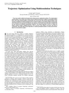
Fig. 1. Robot ABB IRB 6400FHD with 6 degrees of freedom
where β=20, γ=15 and δ=20 are weighting coefficients (the coefficients were set after suboptimal solution investigation). In general, the objective function can contain more criterions. By combining of (10), (11) and (12), we can obtain a universal objective function d) FFcombined = Dtr + βaEtr+ γaTtr+ δaAtr
(13)
In our case the following weights were experimentally set FFcombined = Dtr + 5 Etr+ 10 Ttr+ 5 Atr. 4. CASE STUDY The presented approach has been verified using the simulation model of the industrial robot ABB IRB 6400FHD (Fig. 1). The robot is defined by arm lengths R1 = 0.188 m, R2 = 1.175 m; R3 = 1.3m; R4 = 0.2m; tool: R6x = 0.3; R6y = 0.1 (Fig.2) and by the dynamic parameters listed in Table 1. Using the methodology described above we find the optimal trajectory - operational cycle which is given by ten operational points defined in (14). The robot performs this trajectory as a closed and repeating cycle. The cycle includes the return from P10 to P1 as well. Table 1. Specification of robot motors Motor
Axis rotation[]
E1() E2() E3() E4() E5() E6 (ε)
360 140 165 600 155 600
-180 ; 180 -70 ; 70 -28 ; 105 -300 ; 300 -120 ; 120 -300 ; 300
Rotation velocity [/s] 90 90 90 120 120 190
Rated output [W] 2800 1900 2400 1000 600 500
Energy consum. [W.s/] 31.1 21.1 26.6 8.3 5.00 2.6
Fig. 2. ABB IRB 6400FHD, size in [mm] The defined operating points of the robot are P1 = [2.25;1.1;0.25] P2 = [0.9;1.5;0.25] P3 = [-0.85;1.14;2.22] P4 = [-1.8;1.25;1.17] P5 = [1.8;1.25;1.17] P6 = [-1.25;-1.1;0.25] P7 = [-2.25;-1.48;0.25] P8 = [0.45;-1.14;2.22] P9 = [0.8;-1.25;2.35] P10 = [0.8;-1.25;-1.35].
(14)
4.1 Direct kinematics The robot end effector trajectory is described in a clockwise coordinate system using the transformation matrix (TM) TM = A*B*C*D*E*F*G*H*I
1750
(15)
19th IFAC World Congress Cape Town, South Africa. August 24-29, 2014
where the matrices A, B, C, D, E, F, G, H, I are defined in Table 2.
seconds (see Tab.11). This solution is inefficient from the point of view of energy or the sum of rotation criterions. The sum of the rotation was 50.12 rad and the power consumption per cycle was 53.32 Ws.
The coordinates (x,y,z) of the robot end-effector are given as [ ]
[
]
(16)
In the case of the minimum-rotation control strategy, the best result achieved was the sum of all rotations amounting to 19.74 rad. This solution is close to the combined-optimal control case (Tab. 10). Table 3. Joint rotations for the time-optimal control
4.2 Individual representation Each individual of the GA population is in form (2) and has 6 x 10 = 60 items (genes) which corresponds to 6 rotation angles for reaching of each working point. The ranges of all genes are defined in column 2 of Tab. 1. Note that a singular configuration cannot appear due to the definition of this task. Table 2. Direct kinematics – transformation matrixes Rotation (
(
(
)
(
)
[rad] -0.153 0.603 -0.369 -0.149 -0.475 0.395 -0.398 -0.235 -0.489 0.364
[rad] 2.120 3.128 2.939 2.502 1.899 4.907 3.849 3.221 3.385 3.809
[rad] 0.874 0.229 0.680 0.264 1.307 0.919 0.518 0.679 0.591 0.309
ε [rad] 1.620 1.147 -2.327 -1.130 0.695 -4.978 0.965 -1.798 -0.946 -0.435
Table 4. Objective functions for time-optimal control
)
(
(
)
[rad] 0.720 0.029 -0.142 0.187 0.526 0.110 0.824 -0.269 -0.015 1.222
(
Movement
P1 P2 P3 P4 P5 P6 P7 P8 P9 P10
[rad] 0.345 1.083 2.124 2.453 0.398 -2.184 -2.464 -1.256 -1.001 -0.922
P1 P2 P2 P3 P3 P4 P4 P5 P5 P6 P6 P7 P7 P8 P8 P9 P9 P10 P10 P1
)
)
(
)
)
(
)
(
Tp2p [s] 0.807 0.481 0.663 0.210 1.309 1.643 0.505 0.769 0.162 0.787 7.336
Ap2p [rad] 6.596 5.420 4.716 2.427 5.495 11.806 4.647 4.618 1.525 2.875 50.123
Ep2p [Ws] 6.905 5.806 5.626 2.657 4.617 13.418 5.144 5.260 1.780 2.111 53.324
14.308 11.708 11.004 5.293 11.421 26.867 10.297 10.647 3.467 5.773 110.783
)
Table 5. Joint rotations for minimum-rotation control
4.3 Results and discussion The selected terminating condition of the GA represents the calculation of the predefined number of generations. Experimentally, the value has been set up to 750,000 generations. The obtained results for the time-optimal control are shown in Tab. 3-4, for the minimum-rotation control in Tab. 5-6, for the energy-optimal control in Tab. 7-8 and for the combined control in Tab. 9-10. The goal of the time-optimal control is to achieve the shortest time of the operation cycle. The best result achieved was 7.33 1751
P1 P2 P3 P4 P5 P6 P7 P8 P9 P10
[rad]
[rad]
[rad]
[rad]
[rad]
ε [rad]
0.473 1.026 2.086 2.523 0.597 -2.417 -2.465 -1.087 -0.951 -0.966
0.592 0.293 -0.014 0.179 0.179 0.179 0.794 -0.189 -0.100 1.188
-0.230 -0.008 -0.270 -0.270 -0.270 0.434 -0.459 -0.462 -0.462 0.215
0.130 0.132 2.890 2.890 2.890 2.887 1.342 0.324 0.130 0.130
0.008 1.155 1.155 -0.440 -0.440 -0.665 -0.665 -0.665 -0.526 0.008
-0.617 -0.617 -0.617 -0.617 -0.617 -0.617 -0.617 -0.617 -0.617 -0.617
19th IFAC World Congress Cape Town, South Africa. August 24-29, 2014
Table6. Objective functions for minimum-rotation control P1 P2 P2 P3 P3 P4 P4 P5 P5 P6 P6 P7 P7 P8 P8 P9 P9 P10 P10 P1
Tp2p [s]
Ap2p [rad]
Ep2p [Ws]
0.817 0.488 1.174 0.679 1.093 1.710 0.658 0.782 0.083 0.731 8.214
1.830 1.641 3.238 1.642 1.421 2.913 2.290 2.497 0.412 1.856 19.740
0.963 1.187 1.249 1.295 0.328 0.797 1.224 1.530 0.255 1.840 10.669
Table 10. Objective functions for the combined control
3.610 3.316 5.661 3.616 2.842 5.421 4.171 4.809 0.749 4.427 38.623
P1 P2 P2 P3 P3 P4 P4 P5 P5 P6 P6 P7 P7 P8 P8 P9 P9 P10 P10 P1
Tp2p [s]
Ap2p [rad]
0.910 0.385 0.739 0.229 1.226 1.848 0.642 0.898 0.086 0.642 7.604
2.574 2.084 2.338 0.982 1.929 4.702 1.749 2.452 0.378 1.786 20.974
Ep2p [Ws] 0.581 1.267 0.724 0.586 0.390 1.325 0.996 1.594 0.261 1.213 8.938
4.066 3.736 3.801 1.797 3.545 7.875 3.387 4.944 0.724 3.641 37.517
Table 7. Joint rotations for the energy-optimal control
P1 P2 P3 P4 P5 P6 P7 P8 P9 P10
[rad] 0.302 0.766 1.883 2.318 0.689 -2.312 -2.545 -1.194 -1.011 -1.011
[rad] 0.788 0.246 -0.065 0.415 0.415 0.415 0.746 -0.222 -0.116 0.788
[rad] -0.258 0.437 -0.489 -0.424 -0.181 0.741 -0.351 -0.489 -0.489 0.575
[rad] -1.032 -1.411 -1.411 -1.410 0.371 0.371 0.370 -0.053 -0.205 -0.210
[rad] -0.871 -0.956 -0.959 -1.016 -1.044 -1.044 0.010 0.010 0.010 0.010
ε [rad] 3.198 3.198 3.198 3.198 3.198 3.198 3.198 3.198 3.198 3.198
Table 8. Objective functions for energy-optimal control P1 P2 P2 P3 P3 P4 P4 P5 P5 P6 P6 P7 P7 P8 P8 P9 P9 P10 P10 P1
Tp2p [s] 0.836 0.443 0.711 0.306 1.037 1.910 0.695 0.860 0.117 0.677 7.592
Ap2p [rad] 3.849 2.165 2.359 1.036 3.681 3.923 2.709 2.879 0.441 1.973 25.015
Ep2p [Ws] 1.115 0.906 0.681 0.608 0.761 0.669 1.232 1.336 0.175 1.127 8.609
5.800 3.514 3.751 1.951 5.479 6.502 4.636 5.075 0.733 3.777 41.217
Table 9. Joint rotations for the combined control
P1 P2 P3 P4 P5 P6 P7 P8 P9 P10
[rad] 0.459 0.957 2.118 2.473 0.547 -2.356 -2.519 -1.109 -0.974 -0.971
[rad] 0.590 0.027 -0.180 0.179 0.179 0.179 0.756 -0.286 -0.186 0.590
[rad] -0.123 0.482 -0.489 -0.221 -0.221 0.661 -0.347 -0.347 -0.347 0.661
[rad] -2.397 -2.397 -2.397 -2.397 -2.395 -2.037 -2.037 -2.037 -2.037 -2.037
[rad] -0.014 -0.432 -0.432 -0.432 -0.431 0.128 0.128 0.128 -0.014 -0.014
ε [rad] -0.588 -0.588 -0.588 -0.588 -0.588 -0.588 -0.588 -0.588 -0.588 -0.588
The energy-optimal task has achieved 8.6089 Ws. In this case, it is possible to see the strong correlation between the energy and the time-optimal trajectory. The energy-optimal control is relatively fast (only about 3.5% slower than the fastest trajectory) and also relatively efficient in terms of sum of rotations (26.7% increase in comparison to the rotationoptimal solution). The last case was aimed at finding a combined-control strategy. It includes all the components representing accuracy, operation time, sum of rotations and energy consumption. This solution is fast (only about 3.7% slower than the fastest trajectory), it obtains a good value of rotations (6.3% higher than the rotation-optimal case) and a low power consumption (3.8% higher in comparison with the energyoptimal solution). The evolution of the objective functions of all optimization cases is depicted in Fig. 3, Fig.4 and Fig.5. Table 11. Comparison of all objective functions Objective function Time Rotation Energy Combined
Tp2p [s] 7.3357 8.2136 7.5924 7.6044
Ap2p [rad] 50.1233 19.7401 25.0154 20.9742
Ep2p [Ws] 53.3236 10.6689 8.6089 8.9381
In Fig. 5 the comparison of the evolution of the positioning accuracy in each optimization strategy is compared.
5. CONCLUSION In the proposed robotic arm trajectory optimization, various design aspects have been considered, like operation-time minimization, robot rotation minimization, energy consumption minimization and combined optimization. Because the inverse kinematics task for a robot with many degrees of freedom is a complex problem, the genetic algorithm approach in combination with the robot simulation 1752
19th IFAC World Congress Cape Town, South Africa. August 24-29, 2014
has been proposed. The results obtained have shown that such a design is able to provide very good results and it can achieve significant time savings, energy and wear and tear on the equipment.
ACKNOWLEDGEMENT This project was supported by the Slovak research and grant agency, grant No. VEGA 1/0178/13 and VEGA 1/2256/12. REFERENCES
Fig. 3. Graphs of the objective function evolution for the time-optimal (TO) and rotation-optimal (AO) solution
Fig. 4. Graphs of the objective function evolution for the energy-optimal (EO) and combined-optimal (CO) solution
Davidor, Y. (1991). Genetic Algorithms and Robotics, a Heuristic Strategy for Optimization. World Scientific Eiben, A.E., Smith, J.E. (2007). Introduction to evolutionary computing. Springer. Garg, D.P., Kumar, M. (2002). Optimization techniques applied to multiple manipulators for path planning and torque minimization. Engineering Applications of Artificial Intelligence 15, Elsevier, 241–252 Goldberg, D.E. (1989). Genetic algorithms in search, optimisation and machine learning. Addison-Wesley. Juang, J.G. (2004). Application of Repulsive Force and Genetic Algorithm to Multi-manipulator Collision Avoidance. http://ascc2004.ee.mu.oz.au/proceedings papers/P142.pdf Pac M., Rakotondrabe M., Khadraoui S., Popa D., Lutz P. (2013). Guaranteed Manipulator Precision via Interval Analysis of Inverse Kinematics. In IDETC/CIE 2013 August 4-7, 2013, Portland, Oregon, USA Park, J.H., Kim, H.S., Choy, Y.K. (1999). Optimal Trajectory Control for Robot Manipulators using Evolution Strategy and Fuzzy Logic. In ICASE: Institute of Control, Automation and System Engineering, Korea, June, 1999 Pires S., E.J.,Machado T., J.A., Oliveira De M., P.B. (2004). Robot Trajectory Planning Using Multi-objective Genetic Algorithm Optimization. In GECCO, LNCS 3102, pp. 615–626, Springer-Verlag Berlin Heidelberg Rana, A. S., Zalzala, A. (1997). Collision-free motion planning of multi-arm robots using evolutionary algorithms. In Proceedings of the Institution of Mechanical Engineers Part I, 211, 373–384. Sekaj, I. (2011). Control algorithm design based on evolutionary algorithms. In: Chugo, D., Yokota, S. (ed.), Introduction to Modern Robotics. iC. Press, Hong Kong. iConcept Press Ltd., 2011. - ISBN 978-0980733068. S. 251-266 Virgala I., Frankovský P., Kelemen M. (2013). Mathematical model of a planar manipulator. In: Strojárstvo. Strojárstvo Extra (In Slovak). - ISSN 1335-2938. - Vol. 17, NO. 5 (2013), pp. 140-144.
Fig. 5. Graphs of the positioning accuracy evolution of all optimization strategies.
1753