Using Trajectory Optimization to Minimize Aircraft Noise Impact Mengying ZHANG1; Antonio FILIPPONE; Nicholas BOJDO School of Mechanical, Aerospace, Civil Engineering Manchester M13 9PL United Kingdom
ABSTRACT A multi-objective trajectory optimization framework based on the genetic algorithm has been developed to minimize environmental impact (noise and exhaust emissions). First, a parameterization method is established for the departure phase, with constraints considered for the actual flight scenarios. Second, a lateral parameterization method based on a Bézier spline has been proposed to decrease the number of free parameters. Then a comprehensive flight mechanics program was used to evaluate the aircraft noise impact and to provide the value of the cost functions. Finally, the non-linear optimal control problem is discretized and transformed into a parameter optimization problem that can be solved by a non-gradient optimization procedure. Numerical examples are presented to demonstrate the capability and applicability of proposed technique for a commercial airplane operating out of an international airport. Results show that the framework proposed is effective and flexible. Keywords: Aircraft Noise, Trajectory Optimization, Multi-Objective Optimization I-INCE Classification of Subjects Number(s): 52,60,67,68,76
1. INTRODUCTION The past few decades have witnessed the adoption and acceptance of policies and regulations to control noise exposure and exhaust emissions. However, a compromise between community expectations and the sustainable development of commercial aviation market remains a considerable challenge. As shown in Table 1, although the population within the 57 dBA contour for the four largest airports in the UK has fallen by about 30% in the 14 years ending in 2011, the public still tends to believe that the noise impact has become worse rather than better (1). This negative attitude has placed enormous pressure on airport expansion projects aiming at increasing air traffic capacity; one particularly important example is the debate about Heathrow’s third runway plan (2,3). The problem is not only how to achieve a quieter, cleaner and more efficient operation, but how to compensate the additional environmental cost to support the development of the entire aviation industry. Although the potential of eliminating the environmental pressure from aviation activities with novel engines and aircraft configurations seems promising, solutions with the existing fleet and the technology should not be underestimated. New air traffic management concepts have been aroused in the United States under the name of NextGen (4), in Europe under the name of SESAR (5) and in Japan under the name of CARATS (Collaborative Actions for Renovation Air Traffic Systems) (6), with the aim of satisfying increasingly diverse requirements of airlines and passengers to relieve the pressure in an environmentally friendly way. Previous studies have shown that aircraft noise influence towards communities near the airport can be significantly reduced by difference trajectory operation (8–10). A trajectory optimization tool named NOISHHH developed by Visser et al. (11,12) has integrated a noise model, a geographic information system and a dynamics trajectory optimization algorithm with the collocation method to convert the continuous optimal control problem into a finite-dimensional nonlinear programming problem (13). Similarly, this type of algorithms has also been implemented in the optimization methodology 1
[email protected] (corresponding author).
developed by Hartjes et al. (14) to solve multi-event aircraft trajectories. A multi-criteria optimization strategy with the lexicographic- egalitarian technique is applied by Prats et al. (15,16) to minimise the noise annoyance in Noise Sensitive Areas (NSA). A further study of Khardi et al. (17) demonstrates that the direct method is more appropriate for solving trajectory optimization problems for minimum noise. Table 1 - Changes to Designated Airport Noise Contours (7). Year Airport Heathrow Gatwick Manchester Stansted TOTALS
Number of aircraft movements 441,200 240,200 161,800 102,200 945,400
1998 Area of 57dBA contour [km2] 163.7 76.8 53.5 64.5 358.5
Population within 57dBA contour 341,000 9,000 44,700 7,600 402,300
Number of Aircraft Movements 480,906 251,067 158,300 148,317 1,038,590
2011 Area of 57dBA contour [km2] 108.8 40.4 30.2 21.2 200.6
Population within 57dBA contour 243,300 3,060 27,500 1,300 275,160
The methods mentioned above fall into the category of the gradient-based or derivative-based methods; difficulties occur when dealing with optimization problems for discontinuous models. With the increasing complexity of current optimization problems, there is no guarantee that the integrated problems can always be constructed with continuous models and be differentiable. This has led to the use of heuristic algorithms that are less computationally competitive, but do not need the gradient information; which makes them more suitable to global optimal. A multi-objective mesh adaptive direct search (multi-MADS) method studied by Torres et al. (18) aims to minimise noise and Nitrogen oxides (NO x) emissions for departing aircraft. Yu et al. (19,20) conducted state parameterization with Bernstein polynomials to transform the infinite-dimensional optimal control problem into a finite-dimensional parametric optimization problem to minimise noise impact for arrival trajectories by the genetic algorithm. Similarly, Hartjes & Visser (21) applied the genetic optimization algorithms as well to plan departure flight path for noise abatement and emission reduction. However, constrained by a large number of free parameters for the problem evaluation, the computational efficiency of the genetic algorithms usually gains a less optimistic view. Moreover, when considering additional environmental concerns or different noise attributes, an optimal solution cannot be uniquely selected from the solution of multi-objective optimization problems. In this study, a trajectory optimization method based on genetic algorithm is developed. A new parameterization method is implemented to discretize the flight dynamics equation on both vertical and lateral motion planes to limit the number of free parameters. An aggregated preference value method is applied to pick up the optimal solution among the Pareto solution set as the posterior processing. The details of the problem formulation, including the description of the multi-objective trajectory optimization problems for noise impacts minimization, are explained in §2. The following two sections describe the parameterization method with its implementation, and the posterior selection strategy for the optimized solution. A numerical example demonstrates the noise-optimized departure trajectory from Manchester Airport. The aircraft flight mechanics, aerodynamics, propulsion and acoustic models are built based on the Airbus A320-211 with CFM56 engines.
2. PROBLEM DESCRIPTION 2.1 Objectives Model Various objectives such as flight duration, fuel burn, noise, emissions can be set as the optimization objectives for the flight trajectory. For the assessment of aircraft noise, the comprehensive flight mechanics software FLIGHT (22–24) provides modules to evaluate different indexes of NSAs, such as the EPNL (Effective Perceived Noise Level), SEL (Sound Exposure Level), (A-weighted maximum noise level), awakening ratios, and other metrics. Apart from the physical measurement quantifying environmental impacts, an integrated index to evaluate the financial cost of fuel consumption and exhausts emissions is given in Eq. (1). Instead of summing different objectives with the weighted method, this model transforms the fuel consumption, the total amount of CO 2 emissions and the NO x emission under 3,000 feet (25) into a common metric:
EC = UCfuel ⋅ F +UCCO2 ⋅ CO 2 +UC NOx ⋅ NO x
(1)
where EC denotes the environmental cost of fuel and emissions, UC is the unit cost: for the fuel consumption, it is the unit jet fuel price; for the gaseous emissions, environment-related taxes are adopted.
2.2
Aircraft Flight Dynamics Model A constrained trajectory optimization problem is constructed with aircraft flight dynamics model, constraints of air traffic safety issues, cost functions of different objectives. In general, an aircraft can be modelled as a rigid body with varying mass, aerodynamic, propulsive and gravitational forces. To simplify the problem some assumptions are made: (1) flat and non-rotational earth, (2) no wind, (3) all force acting on the aircraft through its center of gravity, (4) zero angle between the engine thrust and the longitudinal axis of the aircraft, (5) small angle of attack . Thus, a 3 degree-of-freedom flight dynamics model with a set of differential algebraic equations with a variable mass can be simplified as: V& = ( FN − mg sin γ − D) / m γ& = ( L cos µ − mg cos γ ) / ( mV ) χ& = L sin µ / (mV cos γ ) x& = V cos γ sin χ y& = V cos γ cos χ h& = V sin γ m& = − f
(2)
where the state variables consist of true airspeed V, flight path angle , heading angle , bank angle , , the angle of attack , and the three-dimensional location parameters , , ℎ. The thrust force bank angle are the control variables. Other variables include the aerodynamics lift , the drag , the fuel flow . To define the propulsion force and the fuel flow, models based on FLIGHT (24) are introduced as FN = FN (h, Ma, N1 )
(3)
f = f (h, Ma, N1 ) (4) where is the Mach number, is the engine rpm with the value range [70%,103%] for the departure phase. Similarly, the calculation of the aerodynamics coefficients and is also achieved by the software FLIGHT based on flight state variables, the configuration of Airbus A320-211 and custom-defined atmosphere parameters. 2.3 Operational Constraints This section discusses the constraints for the safety and feasibility requirements. First, for a departure, there is neither descent nor deceleration γ ≥0 (5) V& ≥ 0
(6)
Second, to comply with safety and air traffic management, path constraints for the state variables are set
Vstall < V ≤ 250kt
(7)
h0 ≤ h ≤ 10,000ft (8) Sharp turns are not allowed, therefore, the radius of turn and the bank angle are constrained by R = V 2 / g n 2 − 1 ≥ Rmax
where
= /(
−1
2
µ = tan (V / ( gR )) ≤ µ max
) is the load factor, and
!"
= # $ /( %
(9) !"
$
− 1).
(10)
In order to define the initial and final conditions, the following boundary constraints are given:
h(t0 ) = h0 , x(t0 ) = x0 , y (t0 ) = y0
(11)
h(t f ) ≤ hmax , x(t f ) = x f , y(t f ) = y f
(12) where ( ( , ( ) is usually chosen from the coordinates of the waypoints where the aircraft leaves the controlled airspace.
3. PARAMETERIZATION 3.1 Decoupling of the Dynamics Equation Some assumptions are introduced to decouple the three-dimensional model into two motion planes. First, the force normal to the flight path is assumed to be in equilibrium, which leads to * = 0 at each time step and the equation to obtain the lift coefficient
CL = mg cos γ / ( 12 ρV 2 S cos µ )
(13)
where , is the atmospheric density, and - is reference area. With a parabolic drag polar, the drag force is D = (CD 0 (h,V ) + k (h,V )CL 2 ) ⋅ 12 ρV 2 S (14) where . and / are the drag coefficients that can be obtained by the embedded module of FLIGHT. becomes explicit and is no longer an unknown variable. With Eq. (13) and (14), the angle of attack Instead, the flight path angle would become a control variable, along with other two controls: the engine rpm and the bank angle to form the new control vector 0 = [ , , ]3 . Thus, the motion described in Eq. (2) can be decoupled in the vertical plane and horizontal plane respectively:
Horizontal: χ& = g tan µ / V Vertical: x& = V cos γ sin χ y& = V cos γ cos χ
V& = ( FN − mg sin γ − D) / m & h = V sin γ m& = − f
(15)
3.2 Horizontal Track Parameterization Among those horizontal track parameterization methods, waypoints are usually used to define the departure routes. The lateral tracks can be expressed by a series of waypoints enable to construct the flight path between each two waypoints. Two different types of legs – track-to a-fix (TF) legs and radius-to-a-fix (RF) legs – are highly preferred which means the lateral trajectories is built with straight legs and constant radius turns (26–28). Trajectory models defined by spline interpolation have also been developed and introduced (29). Conventionally, the first methods are adopted for the ease of implementation of the constraints from existing operational requirements and air traffic guidance. However, with the development of the technology of today’s navigation and guidance, a far more complex situation could be handled with the increased airspace complexity caused by optimized free flight routes. In this paper, a parameterization method using a Bézier curve is used to obtain the horizontal track. Bézier polygon
Figure 1 - Bézier curve with in the Bézier polygon.
is the order of A Bézier curve is defined by a set of control points 4. ( . , . ) to 45 ( 5 , 5 ), where the curve. The property that the first and last control points are the end points on the curve yet the intermediate control points generally are not on the curve makes Bézier curve ideal to describe the aircraft ground track. Another property is that the convex hull of the Bézier polygon would wrap around the Bézier curve, Figure 1. For a given population density distribution around the airport, a noise abatement ground track could be designed within the Bézier polygon to approximate the ground corridor steering clear of the NSAs. The form of the curve is given by n
B(t ) = ∑ bi , n (t )Pi , t ∈ [0,1], i = 0,..., n
(16)
i =0
where the polynomials
n bi ,n (t ) = t i (1 − t )n −i , i = 0,..., n (17) i are known as Bernstein basis polynomials of degree ; 78 are the coordinate of the control points. The curvature radius (9) on the curve is obtained from 3 ( x '2 (t ) + y '2 (t )) 2 R(t ) = (18) x '(t ) y ''(t ) − x ''(t ) y '(t ) The bank angle could be determined by the same equation shown in Eq.(10). Note that the positive sign represents turning right and the negative indicates turning left. Therefore, the control is explicitly expressed by the coordinate of the control points 78 which define the lateral variable track.
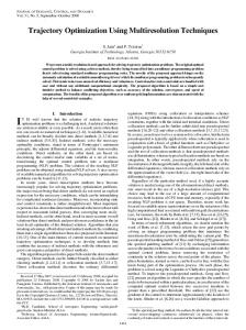
3.3 Vertical Profile Parameterization In order to simplify the problem, the departure procedure is split into segments consisting of climb and acceleration, see for example Figure 2: two accelerations (i.e. AB and CD) and two constant speed climb (i.e. BC and DE) are assumed. The focus would be put on the parameters that describe the climb profile and their effect on the noise perceived at the NSAs. Detailed explanations of parameterization have been published (29). Description of each segment with the vertical free parameters is given in Table 2.
Figure 2 - Take-off and climb-out (31). Table 2 - Description of flight segments. Segment
Description
Free Parameters
AB
full trust acceleration while climbing
BC
constant climb
γ A , VB , hB γB
CD
level acceleration
VD , N1CD
DE
climb/level flight
γD
In summary, the 3D departure trajectory can be parameterized through two sets of free parameters: horizontal free parameters :;?E B in Table 2. Figure 3 demonstrates the computation procedure of the 3D flight dynamics model; this is controlled by the free parameters through three variables, namely the engine rpm , the flight path angle and the bank angle .
p horizontal
p vertical
& g tan µ χ = V x& = V cos γ sin χ y& = V cos γ cos χ
V2
µi = ± tan −1 ( i ), gRi N1i , γ i
& FN − mg sin γ − D V = m & h = V sin γ m& = − f
xi +1 = [V , χ , x, y , h, m]i +1T
i = i +1
Figure 3 - Computation procedure of 3D flight dynamics model.
4. POSTERIOR SOLUTION SELECTION More complicated problems will arise when multiple significant attributes (e.g. flight time) are considered in the same problem. In order to provide an intuitive and understandable way to select the optimized solution, a method to evaluate the various departure procedures using the decision maker (DM)’s preferences is developed. Firstly, preference types of different attributes or criteria are defined. Subsequently, essential knowledge and concerns from the DMs are translated into preference functions within separate ranges. Finally, an aggregated preference function is built to generate a single metric for evaluation. By comparing these values between various objectives, the optimal solution can be selected from the solution set. In the theory of physical programming (32), the sharpness of the preference would define the types of different criteria. The objectives in this paper can be attributed to one of the classical three types: type-1, smaller is better. For each criterion, ranges are used to express the level of desirability towards the criteria. Numerical values of the F GH criterion 8 ( ) at the boundaries of these ranges, I 8 (F = 1, … , ; / = 0,1, … , ), are used to quantify the preferences in ascending order. This means a higher preference for the first value and lower for the last one. Usually, it is highly dependent on the experiences and knowledge of the experts to define the value ranges. One example of desirability with = 5 is described in Table 3 with its preference function depicted in Figure 4. Table 3 - Preferences order and attribution with Level Description A Highly desirable B Desirable C Tolerable D Undesirable E Highly undesirable
Type-1 < 8≤ < 8 ≤ 8 $ < 8 ≤ 8 O 8 < 8 ≤ P 8 < 8 ≤ . 8
8 $ 8 O 8 P 8 Q 8
= 5.
ni ( x)
α5
α4 α3 α2 α1 α0 fi 0
f i1
fi 2
fi 3
fi 4
f i 5 f i ( x)
Figure 4 - Preference function type-1 with = 5(33). To evaluate the different objectives under a common metric, in each range the same set of images I is used to construct the preference function, no matter what the preference type or criterion is. The images I at the boundaries 8I are calculated from I
=T
IU
0, ∙ 858 ,
/=0 1≤/≤
(19)
Note that I is a set of dimensionless parameters to develop the preference functions with a piecewise exponential function (34). For the general / GH range, 8IU < 8 ( ) ≤ 8I , the preference function with order is defined as
WI ( ) =
The value of WI at the boundary
I 8
WI ( ) =
IU
is
+ YI Z1 − I,
Z
(20)
hence
YI = IU
( (")U(]^_` U5\ ] ^ ^_` a (] U(] [
− IU |1 − [ U5 | I
+ YI Z1 −
(21)
( (")U(]^_` U5\ ] ^ ^_` a (] U(] [
Z
(22)
Therefore, the type-1 preference function for the F GH criterion can be defined as
. 0, 8( ) < 8 IU (23) ≤ 8 ( ) ≤ 8I 8 ( ) = c WI ( ), 8 W ( ), 8( ) > 8 where 1 ≤ / ≤ and W ( ) = . Once the preference functions in each range for different objectives are constructed, an aggregated preference function #( ) could be established as Eq. (24). The decision-making process is to find the option with the minimum #( ): f
#( ) = e 8g
8(
)
(24)
5. NUMERICAL EXAMPLE AND RESULTS An Airbus A320-211 departing southwest from runway 23R/05R in Manchester Airport (25) in the UK is chosen to demonstrate the capability of the method proposed. The closest residential community near the end 23R is the town of Knutsford (coordinates:53.30< N, 2.371< W). The departure trajectory is to be optimized for minimum noise and minimum environmental impact: J1 = EPNL, J 2 = EC
(25)
Since the reference point is located in the coordinate of runway’s end, the initial condition of the departure point is . = −916.7118m, . = −399.5492m, ℎ. = 3m, #. = 75m/s. The end point is selected with the reference of an existing instrumental departure routing, with the end-point fixed at ( = −18119.1951m, ( = −16708.6863m. Then the lateral track to be optimized is segmented into two phases: the initial straight leg and the next Bézier curve segment with one control point, leading to :;?