excitation of Lamb waves by single longitudinal and shear type transducers has bean determined using ..... selected relatively big to be in a far field zone of the.
ISSN 1392-2114 ULTRAGARSAS (ULTRASOUND), Vol.62, No.4, 2007.
Optimization of transducer arrays parameters for efficient excitation of Lamb waves L. Mažeika, R. Kažys, A. Maciulevičius Ultrasound institute of Kaunas University of Technology, Abstract: The guided waves are used for inspection of large industrial constructions. The Lamb waves are a sort of the guided waves propagating in planar structures. They can be used for inspection of such objects like metal plates and sheet piles. The regularities of the excitation of Lamb waves by single longitudinal and shear type transducers has bean determined using numerical modelling. The directivity patterns of the transducers arrays having different configurations have been investigated using the results of the numerical modelling. It was found out that the main problem is not the generation of guided waves, but generation of the desired mode of a guided wave. In the case of generation of various modes under the different angles to the main wavefront direction, it is complicate to interpret the results because the waveforms of the received signal become very complicated. The obtained results revealed several configurations of the transducer arrays which enable generation only the desired mode of the Lamb wave with a relatively low level of the parasitic, e.g., undesired waves. It was also demonstrated and explained the difference between application of the longitudinal and the shear type of the transducers in ultrasonic arrays. It was pointed out the advantage of the delay time technique of excitation of transducer arrays comparing to the simultaneous excitation of all elements of the array. Key words: transducer arrays, Lamb waves, directivity pattern, modelling.
•
Introduction The guided waves are used or can be used for inspection of large, elongated industrial objects such like pipes, rails, cable ropes and etc [1-4]. The Lamb waves are a sort of the guided waves which propagate in planar components of the objects. In general, propagating guided waves contain all three components of particle velocity. The different combinations of the amplitudes and phases lead to the existence of many modes. So, selective generation of the desired guided waves mode can be implemented by excitation of the specific components of the displacements (or particle velocities), matching them to the spatial and temporal properties of the desired wave. This can be implemented only exploiting a priori knowledge about properties of propagating guided waves and the characteristics of the used transducer. The most promising technique for generation of the selected modes is application of transducer arrays, because most of the long range ultrasonic inspection objects are plate - like structures, such as plates, sheet piles, pipes. So, the investigation presented below is devoted to determination of the regularities of the guided wave generation in plates using transducers arrays. The main problem is optimization of the transducer array used for generation of a desired mode of guided waves. The optimization means that should be developed such a transducer array which most efficiently generates desired waves along the object and at the same time it creates a low level parasitic side lobes. The investigations were carried out in the following steps: • The investigation of the regularities of the excitation of the Lamb waves using the single longitudinal waves and shear waves transducers; • The analysis of the directivity patterns of the transducer arrays having different configurations and based on the different types of transducers (longitudinal and shear);
Comparison of the different techniques of the transducer array excitation: simultaneous and using the time delay.
The point spread function of the point source of longitudinal and shear waves In the most cases of applications of the long range ultrasonic the dimensions of the transducers are smaller comparing to the wavelength of the excited guided waves. So, it can be assumed that the transducers are point like sources of ultrasonic waves having a wide or even a circular directivity pattern. The objective of this step was to investigate the directivity patterns of the longitudinal and the shear type point sources using the 3D finite element modelling and to estimate how efficiently the A0 and the S0 modes of Lamb wave are generated using the different types of transducers. The investigation has been carried out using finite element model of the aluminium plate (Fig.1). The aluminium parameters are presented in the Table 1. The dimensions of the plate are 0.5x0.5m and the thickness 10mm. Table 1. The parameters of the aluminium used in the modelling Parameter
Value
Density, ρAl
2700 kg/m3
Young modulus, EAl
70 GPa
Poisson’s ration, ν
0.33
For the excitation the 2 periods burst having the Gaussian envelope and the frequency 70 kHz was used. The waveform of the excitation signal is presented in Fig.2. Such a narrowband signal was selected with the purpose to have a better selectivity of the different wave modes propagating with different velocities. Two types of excitation have been analysed: the normal to the surface of
7
ISSN 1392-2114 ULTRAGARSAS (ULTRASOUND), Vol.62, No.4, 2007. the plate (longitudinal) (Fig.1a) and the tangential (shear) (Fig.1b). The excitation force was added in the middle of the aluminium plate.
propagating to the right in Fig.4.. The distribution of the tangential component of a particle velocity vτ = v x2 + v 2y at the time instant 50 μs after excitation presented in Fig.5 demonstrates the similar features of the S0 mode Lamb wave also.
Excitation point
z
a y x
Excitation point
10mm
0.5m b
0.5m
Fig.1. Investigated aluminium plates: a - the normal excitation force; b - the shear excitation force
uex (t), a.u.
Fig.3. The distribution of the modulus of a particle velocity of the A0 mode wave at the time instance 75μs after the excitation using the longitudinal waves point like transducer.
1 0.8 0.6 0.4 0.2 0 -0.2 -0.4 -0.6 -0.8 -1
0
10
20
30
40
t, μs
Fig.2. The waveform of the excitation signal
In the case of the normal excitation the task in principle is axi-symmetric and as a consequence the directivity patterns of both A0 and S0 modes are uniform in all directions (circular). This is demonstrated by the distribution modulus of the particle velocity
Fig.4. The distribution of the normal particle velocity
v z ,t =50 (x, y )
of the A0 mode wave at the time instance 50 μs after the excitation using the shear wave point like transducer.
v = v x2 + v 2y + v z2 at the time instant 75μs after excitation,
The directivity patterns of the tangential point source for the A0 and the S0 modes of Lamb waves were calculated using the particle velocity distribution at the time instant 50 μs according the following expressions: d A0 (α ) = max v z , t = 50 (x, y ) , (1)
presented in Fig.3. So, it can be assumed that the point source of longitudinal waves generates the Lamb waves having close to the circle directivity pattern. More complicated is application of the shear type transducers, even if to assume that they are very small comparing to the wavelength. In the case of the tangential excitation the acoustic field have a non-uniform distribution. The distribution of the normal component of a particle velocity (Fig.4) demonstrates that the A0 mode of Lamb waves propagating in the opposite direction have an opposite phase with respect to the phase of the wave
R1, A0 < R < R2 , A0
d S 0 (α ) =
max
R1,S 0 < R < R2,S 0
v xy,t = 50 (x, y ) ,
(2)
where d A0 (α ) , d S 0 (α ) are the directivity patterns of the A0 and S0 modes,
8
ISSN 1392-2114 ULTRAGARSAS (ULTRASOUND), Vol.62, No.4, 2007. v xy ,t =50 (x, y ) = v x,t =50 (x, y ) ⋅ cos(α ) + v y ,t =50 (x, y ) ⋅ sin (α ) ,
x
90° 1
vx ,t = 50 (x, y ) , v y ,t = 50 (x, y ) , vz ,t =50 (x, y ) are x, y and z
120°
60° 0.8
components of the particle velocity at the time instant 50μs, α = arctan(x / y ) , R1, A0 , R1, S 0 , R2, A0 , R2, S 0 are the
y
0.6 150°
30° 0.4
ranges of the A0 and the S0 mode waves along the radius measured from the origin (zero) point.
0.2
-
180°
+
0°
Excitation direction
330°
210°
240°
300° 270°
Fig.7. The directivity pattern
d S 0 (a )
of S0 mode wave in the case of
the tangential excitation obtained from the results of the finite element modelling. The excitation force direction is denoted by the arrow.
Analysis of the directivity patterns of the transducer arrays having different configuration Fig.5. The
In general for calculation of a directivity pattern of the guided waves it is necessary to use the model that enables to take into account dispersion phenomenon. On the other hand in most long range applications generation of the guided waves is performed at the frequencies which are outside strong dispersion ranges. Taking all this into account the simplified directivity pattern calculation technique has been developed. The calculation of the directivity pattern of a transducer array is based on: the known position of the transducer array element xte, k , yte, k , k = 1 ÷ N te , Nte is the
distribution of the tangential particle velocity v xy ,t =50 x, y of the S0 mode at the time instant 50 μs after
(
)
the excitation using the shear waves point like transducer
The obtained directivity patterns are presented in Fig.6 and 7. As can be seen both of them have two lobes in front and back directions having opposite phases. There is a very week generation in lateral direction. x
90° 1 120°
number of the transducer elements; the known group cg and phase cph velocities of the guided waves under analysis. The directivity pattern the transducer array was calculated according to d ta (α ) = max[uΣ (α , t )] − min[uΣ (α , t )] , (3)
60° 0.8
y
0.6 150°
30° 0.4
t
t
0.2
-
180°
where
+
uΣ (α , t ) =
0
Excitation direction
N te
∑ uk (α , t ) , k =1
uk (α , t ) is the signal generate by the kth element of transducer array under the angle α. For calculation of the signal generated at some angle the distance d between the centre of the transducer array OTA (xTA , yTA ) and the observation point OP (xP , y P ) was selected relatively big to be in a far field zone of the transducer array. In the case under analysis it was 5 m. The position of the observation point is calculated according to x P = d ⋅ sin (α ) + xTA . (5) y P = d ⋅ cos(α ) + yTA
330°
210°
240°
300° 270°
Fig.6. The directivity pattern
d A0 (a )
(4)
of the A0 mode wave in the
case of the tangential excitation obtained from the results of the finite element modelling. The excitation force direction is denoted by the arrow.
9
ISSN 1392-2114 ULTRAGARSAS (ULTRASOUND), Vol.62, No.4, 2007. The signals at the observation point given by uk (α , t ) = e
(
− a 2 n p ,t − t P
(
)
a np ,t − t p
where
) ⋅ sin (2πft − Δt
ph
),
one of the modes can be observed almost in all cases. From the presented figures follows that most promising for A0 generation is a horizontal array with a spacing λA0/2 (Fig.10) and the matrix transducer array 2x4 (Fig.15) with the horizontal spacing λA0/2 and the vertical spacing λA0. The selection of the most optimal transducer array is based on the following criteria – the biggest front lobe of the directivity pattern and the smallest side lobes, because side lobes create multiple reflections across the plate. In the case of the horizontal array (Fig.10) the strong generation of S0 occurs also, but side lobes are slightly smaller comparing to the transducer array 2x4. More complicated results are obtained when the distance between transducers corresponds to the wavelength or half wavelength of the symmetric Lamb wave mode S0 (Fig.16-22). The regularities of the directivity patterns of the S0 mode are similar to those which were obtained for A0 (Fig.10-15) with a corresponding distance between transducers. However the directivity patterns of the A0 mode are much more complicated. In all cases (Fig.16-22) the multiple side lobes can be observed. So, it can be stated that in any case of the analyzed transducer arrays except the desired S0 mode always undesired A0 mode waves with a relatively strong amplitude will be generated. The directivity patterns of a few more types of the transducer arrays are presented in Fig.23-24. One of them is more efficient for excitation of the S0, another one of A0 modes and both has relatively low level lobes of the A0 mode. The last one is 2x4 inverted array, that is, the transducer of the second raw are excited using the signals of an opposite polarity. Such a transducer array have one lobe of S0 mode, but several side lobes of A0 mode generated approximately at 45° angle to the main direction. Comparing the amplitudes of the S0 and the A0 modes in the directivity pattern it is necessary to take into account that a true ratio of their amplitudes very depends on the excitation efficiency, which should be determined by a numerical modelling and/or experimentally and was not taken into account in the presented results.
(6)
is the normalization coefficient
dependent on the number of the periods np in the signal and the wave energy propagation time tp , tp = t ph =
(x P − xk )2 + (x P − xk )2 cg
(x P − xk )2 + (x P − xk )2
(
c ph
,
,
)
Δt ph = t ph − t g ⋅ f ⋅ 2 ⋅ π ,
f is the central frequency of the signal. Using this approach the directivity patterns of the different configurations of the transducer arrays consisting of eight elements have been calculated. The velocities of A0 and S0 modes of Lamb waves used in calculations are presented in Table 2. These parameters correspond to the Lamb wave velocities in 10mm thickness aluminium plate at the 70kHz frequency. The directivity patterns were calculated at the distance 5m using the 5 periods burst with the Gaussian envelope. The waveform of the signal is presented in Fig.8. Table 2. The Lamb wave velocities used in the calculations Velocity
A0, m/s
S0, m/s
Phase
2110
5397
Group
3065
5310
u(t) 1 0.8 0.6 0.4 0.2 0 -0.2
90° 1
-0.4
120°
0.8
-0.6 -0.8 -1
0.6
150° 0
50
100
150
200
250
300
60°
30°
0.4
350 t, µs
0.2 Fig.8. The waveform of the signal used in the directivity pattern calculations
180°
It was assumed that a single transducer generates both A0 and S0 modes of the Lamb waves propagating in all direction. Such an assumption is close to reality when the pressure or longitudinal type transducer is used. The obtained directivity patterns of the different types of transducers arrays are presented in Fig.9-15. In the right upper corner of the figures the type of the transducer is denoted. By the solid line is shown the directivity pattern of the A0 mode, by the dashed line – of the S0 mode. As can be seen in most cases both A0 and S0 modes of the Lamb waves are generated. The big side lobes at least of
0°
330°
210°
300°
240° 270°
Fig.9. The directivity pattern of the “horizontal” 8 element longitudinal (excitation normal to the surface) transducer array. The spacing is λA0: solid line – A0, mode dashed line – S0 mode
10
ISSN 1392-2114 ULTRAGARSAS (ULTRASOUND), Vol.62, No.4, 2007. 90° 1 120°
0.8
120°
60°
0.6
150°
0.8
x 30°
0.4 0.2
0.2 180°
180°
0°
0°
330°
210°
330°
210°
300°
240°
300°
240°
y 60°
0.6
150°
30°
0.4
90° 1
270°
270°
Fig.10. The directivity pattern of the “horizontal” 8 element transducer array. The spacing is λA0/2: solid line – A0, dashed line – S0
Fig.13. The directivity pattern of the transducer array 4x2. The spacing along axis x is λA0/2, along y axis is λA0: solid line – A0, dashed line – S0
90° 1 120°
0.8
90° 1
60°
120°
0.6
150°
0.4
0.2
180°
180°
0°
330°
210°
0°
330°
210°
300°
270° Fig.14. The directivity pattern of the transducer array 2x4. The spacing along both axes is equal to wavelength of A0 mode λA0 solid line – A0, dashed line – S0
Fig.11. The directivity pattern of the “vertical” 8 element transducer array. The spacing is λA0: solid line – A0, dashed line – S0
120°
0.8
y 60°
120° 30°
0.4
0.8
y 60° x
0.6
150°
30°
0.4
0.2
0.2
180°
0°
180°
330
210°
0°
330°
210°
300°
240°
90° 1
x
0.6
150°
300°
240°
270°
90° 1
30°
0.4
0.2
240°
x
0.6
150°
30°
0.8
y 60°
300°
240°
270°
270°
° Fig.12. The directivity pattern of the transducer array 4x2. The spacing along both axes is equal to wavelength of A0 mode λA0: solid line – A0, dashed line – S0
Fig.15. The directivity pattern of the transducer array 2x4. The spacing along axis x is λA0/2, along y axis is λA0: solid line – A0, dashed line – S0
11
ISSN 1392-2114 ULTRAGARSAS (ULTRASOUND), Vol.62, No.4, 2007. 90° 1 120°
0.8
120°
0.6
150°
x 30°
0.4 0.2
180°
180°
0°
330°
210°
0°
330°
210°
300°
240°
300°
240°
270°
270°
Fig.16. The directivity pattern of the “horizontal” 8 element transducer array. The spacing is λS0: solid line – A0, dashed line – S0
90° 1 0.8
Fig.19. The directivity pattern of the transducer array 4x2. The spacing along both axes is equal to wavelength of A0 mode λS0: solid line – A0, dashed line – S0
120°
0.8
60° x
30°
0.4
0.6
150°
30°
0.4
0.2
0.2
180°
0°
180°
330°
210°
0°
330°
210°
300°
240°
y
90° 1
60°
0.6
150°
60°
0.6
0.2
120°
0.8
150°
30°
0.4
y
90° 1
60°
300°
240°
270°
270° Fig.20. The directivity pattern of the transducer array 4x2. The spacing along axis x is λA0/2, along y axis is λS0: solid line – A0, dashed line – S0
Fig.17. The directivity pattern of the “horizontal” 8 element transducer array. The spacing is λS0/2: solid line – A0, dashed line – S0
y 90° 1 120°
0.8
120°
60°
0.8
0.6
150°
60° x
0.6
150°
30°
0.4
30°
0.4
0.2
0.2
180°
180°
0°
330°
210°
240°
90° 1
0°
330°
210°
300°
300°
240°
270°
270°
Fig.18. The directivity pattern of the “vertical” 8 element transducer array. The spacing is λS0: solid line – A0, dashed line – S0
Fig.21. The directivity pattern of the transducer array 2x4. The spacing along axis is equal to wavelength of A0 mode λS0: solid line – A0, dashed line – S0
12
ISSN 1392-2114 ULTRAGARSAS (ULTRASOUND), Vol.62, No.4, 2007. y
90° 1 120°
0.8
60°
0.8
x
0.6
150°
180°
0°
Fig.25. The directivity pattern of the inverted 2x4 transducer array. The spacing along axis x is λS0/2, along y axis is λA0: solid line – A0, dashed line – S0
Directivity patters of array in the case of the shear type transducers
y 60° x
0.6
The directivity patterns of the arrays exploiting shear type transducers were calculated taking into account directivity patterns of a single element which were obtained using the finite element modelling. So, the integral signals of A0 and S0 modes at the observation point were calculated according to
30°
0.4 0.2 180°
0°
uΣ, A0 (α , t ) = uΣ, S 0 (α , t ) =
300°
240°
0.8
y 60°
(7)
S0
(a )⋅ uk (α , t ) .
(8)
N te
∑d
90° 1 0.8
x 30°
0.4
60°
0.6
150°
30°
0.4
0.2
0.2
180°
0°
180°
330°
210°
0°
330°
210°
300°
240°
(a )⋅ uk (α , t ) ,
120°
0.6
150°
A0
The obtained directivity patterns for several configurations of transducer arrays are presented in Fig. 26-28. In general, the similar regularities can be observed, except that side lobes are essentially reduced. The side lobes perpendicular to the main direction almost completely disappeared.
Fig.23. The directivity pattern of the transducer array 2x4. The spacing along axis x is λA0/2, along y axis is λS0: solid line – A0, dashed line – S0
90° 1
∑d k =1
270°
120°
N te
k =1
330°
210°
300°v 270°
Fig.22. The directivity pattern of the transducer array 2x4. The spacing along axis x is λS0/2, along y axis is λS0: solid line – A0, dashed line – S0
90° 1
330°
240°
300° 270°
150°
0°
210°
330°
210°
0.8
30°
0.2
180°
120°
x
0.4
0.2
240°
60°
0.6
150°
30°
0.4
y
90° 1 120°
300°
240°
270°
270°
Fig.24. The directivity pattern of the transducer array 2x4. The spacing along axis x is λS0/2, along y axis is λA0: solid line – A0, dashed line – S0
Fig.26. The directivity pattern of the “horizontal” 8 element shear type transducer array. The spacing is λA0: solid line – A0, dashed line – S0
13
ISSN 1392-2114 ULTRAGARSAS (ULTRASOUND), Vol.62, No.4, 2007.
120°
90° 1 0.8
time technique is the possibility to reduce of the amplitude of the backward lobe. The second advantage is that the dimensions of the transducer array are not critical.
60°
0.6
150°
30°
0.4
120°
90° 1 0.8
0.2 180°
0.6
150°
0°
60°
30°
0.4 0.2 180°
330°
210°
0°
300°
240°
Fig.27. The directivity pattern of the “horizontal” 8 element shear type transducer array. The spacing is λA0/2: solid line – A0, dashed line – S0
0.8
300°
240° 270°
90° 1 120°
330°
210°
270°
Fig.29. The directivity pattern of the “vertical” 8 element shear type transducer array. The spacing is λS0: solid line – A0, dashed line – S0
60°
0.6
150°
30°
0.4
90° 1 120°
0.2 180°
0°
0.8
60°
0.6
150°
30°
0.4 0.2 330°
210°
180°
0°
300°
240° 270°
330°
210° Fig.28. The directivity pattern of the “vertical” 8 element shear type transducer array. The spacing is λS0 solid line – A0, dashed line – S0
300°
240° 270°
Comparison of simultaneous excitation of transducer array and excitation using time delay
Fig.30. The directivity pattern of the “vertical” 8 element shear type transducer array. The spacing is λA0/2 solid line – A0, dashed line – S0
In the experiments and calculations presented above it was assumed that all elements of the transducer array were excited at the same instance. The control of the directivity and the efficiency of the transducer array were implemented by changing the distances between the elements. On the other hand, the control of the transducer array can be performed by introducing individual delay times for each element. The objective of this stage of investigation was to determine what difference in the performance of transducer arrays can be expected when one or another excitation technique is used. With the purpose to clarify this question the directivity patterns of a “vertical” transducer array with different spacing were calculated in the case when the delay time technique is used. The obtained results are presented in Fig.29-30. The results demonstrate that the main advantage of the delay
Conclusion The main conclusions of the research carried out are the following: 1. There are two factors that complicate interpretation of the waveforms of received signals: almost in all cases of the arrays both A0 and S0 modes of Lamb waves and also Lamb waves in lateral directions are generated. 2. The “horizontal” transducer arrays in all cases generate both A0 and S0 modes of Lamb waves. Selective generation of only A0 or S0 mode waves can be implemented only by application of “vertical” or matrix transducer arrays.
14
ISSN 1392-2114 ULTRAGARSAS (ULTRASOUND), Vol.62, No.4, 2007. 3.
4.
5.
6.
In the case of the longitudinal type of transducers the smallest side lobes in the directivity patterns possess the following arrays: • the “horizontal” array with the spacing λA0/2 generating A0 and S0 mode waves; • the array 2x4 having spacing λA0/2 in the “horizontal” direction and λA0 in the “vertical” direction generating mainly A0 mode wave; • the array 2x4 having spacing λA0/2 in the “horizontal” direction and λS0 in the “vertical” direction generating mainly S0 mode waves; The arrays with the shear type transducers possess essentially smaller side lobes, comparing with the arrays based on longitudinal type of the transducers, especially in the lateral direction. Due to the simultaneous excitation technique the directivity patterns of all types of transducer arrays are symmetric with respect to both axis (horizontal and vertical). As a consequence, the waves in front and back directions are generated of the same amplitude. The waves generated in the backward direction are reflected by the edge of the plate and complicate interpretation of the results. The application of the delay time excitation technique enables essentially to reduce the amplitude of the signal generated in the backward direction.
Project is coordinated and managed by TWI (UK). Ref.: Coll-CT-2005-516405. References ®
1.
Mudge P. J. Field Application of the Teletest Long-Range Ultrasonic Testing Technique, Insight. 2001.Vol.43. P.74- 77.
2.
Song.W.-J., Rose J. J., Whitesel H. An ultrasonic guided waves technique for demage testing in a ship hull. Materials Evaluation. 2003. Vol.60. P. 94-98.
3.
Cawley P., Lowe M. J. S., Alleyne D. N, Pavlakovic B. and Wilcox P. Practical long range guided wave testing: Applications to Pipes and Rail, Mat. Evaluation. 2003. Vol.61. P. 66-74.
4.
Kwun H., Kim S. Y. and Light G. M. The magnetostrictive sensor technology for long-range guided- wave testing and monitoring of structures. Evaluation. 2003. Vol.61. P. 80-84.
L. Mažeika, R. Kažys, A. Maciulevičius Ultragarsinių gardelių Lembo bangoms žadinti optimizavimas
Reziumė Nukreiptosios bangos naudojamos didelėms pramoninėms konstrukcijoms tikrinti. Plokščiuose objektuose sklindančios Lembo bangos tiktų defektams aptikti metalo plokštėse ar jų gaminiuose. Tokioms bangoms žadinti naudojamos ultragarsinės gardelės. Šio darbo tikslas buvo ištirti įvairios konfigūracijos Lembo bangų žadinimo gardelių kryptines savybes. Baigtinių elementų metodu buvo nustatytos vieno gardelės elemento kryptingumo diagramos išilginių ir skersinių bangų keitiklių atvėjais. Naudojant gautąsias kryptines elementų charakteristikas buvo apskaičiuotos įvairios konfigūracijos aštuonių elementų gardelių kryptingumo diagramos. Jos parodė, kad daugeliu atvejų žadinamos tiek simetrinė S0, tiek asimetrinė A0 Lembo bangų modos. Be to, gana ryškūs yra šoniniai lapeliai. Kaip tyrimų rezultatas buvo nustatytos optimalios gardelių konfigūracijos, įgalinančios žadinti norimą Lembo bangų modą esant minimaliam šoninių lapelių ir parazitinių modų lygiui.
Acknowledgements The part of this work was sponsored by the European Union under the Framework-6 LRUCM project. The
Pateikta spaudai 2007 12 12
15