Then, the model coefficients adopted in the tree canopy models were optimized by comparing numerical results with field measurements of wind velocity and ...
Optimization of Tree Canopy Model for CFD Prediction of Wind Environment at Pedestrian Level Akashi Mochida a, Hiroshi Yoshino a, Tatsuaki Iwata a, Yuichi Tabata a a
Department of Architecture and Building Science, Graduate School of Engineering, Tohoku University, Sendai, Japan
ABSTRACT: The canopy model for reproducing the aerodynamic effects of trees based on k-ε model was optimized for the CFD prediction of wind environment at pedestrian level. After reviewing the previous researches on modeling canopy flows, two types of canopy models were selected. In addition, the model coefficients adopted in the extra term added to the transport equation of turbulence energy dissipation rate, ε were optimized by comparing numerical results with field measurements. KEYWORDS: Tree Canopy Model, Aerodynamic Effects of Trees, Wind Environment 1 INTRODUCTION Tree planting is one of the most popular measures to improve outdoor environment, i.e. avoiding strong gust around high-rise buildings, improving outdoor thermal comfort etc. Thus, an accurate prediction of tree effects is often needed. This study emphasized the modeling of aerodynamic effects of trees, i.e. to decrease the wind velocity but to increase the turbulence. Many tree canopy models proposed for reproducing the aerodynamic effects of trees have been found in literature ([1]~[7]). In this study, the previous researches involved in using tree canopy models was cautiously reviewed and classified. Then, the model coefficients adopted in the tree canopy models were optimized by comparing numerical results with field measurements of wind velocity and turbulent energy k around trees. 2 MODELING FOR TREE CANOPY 2.1 Modeling of aerodynamic effects of tree canopy The canopy models were derived based on the k-ε model in which extra terms were added in the transport equations (cf. Table 1). The extra term “-Fi” added in the momentum equation gives the effect of trees on velocity decrease, whilst the extra terms “+Fk” and “+Fε” included in k and ε transport equations simulate the effects of trees on the amount of increase in turbulence and energy dissipation rate respectively. These extra terms were derived by applying the spatial average to the basic equations ([1]). 2.2 Classification of the extra terms for incorporating aerodynamic effects of tree canopy The tree canopy models proposed in the previous researches ([1]~[7]) can be classified into four types (Types A~D) as shown in Table 1. It can be seen that the same form of “Fi” is used and two different forms of Fk are adopted. The Fk in Types A and B was expressed as follows. Fk=Fi
( < > : ensemble-average)
−561−
(1)
This form was analytically derived by Hiraoka ([1]). In Types C and D, Fk was modified by including an additional sink term, i.e. Fk = Production(Pk) - Dissipation(Dk)
(2)
Pk: production of k within canopy (=Fi) Dk: a sink term to express the turbulence energy loss within canopy (Green [2])
In Types A and D, Fε was formulated by using a length scale “L” within canopy as ⎛ 3 1⎜k 2 τ ⎜⎜ L ⎝
Fε ∝
⎞ ⎟ ⎟⎟ , ⎠
τ = k/ε and L=1/a .
where
(3)
On the other hand, the form of Fε shown in Type B was given as 1
Fk , where τ = k/ε . (4) τ In Type C, the term corresponding to the sink term in Eqn.(2) was added for the expression of Fε. Fε ∝
Fε = Production (Pε) – Dissipation (Dε) ( Pε ∝
1
τ
Dε ∝
Pk
1
τ
(5)
Dk )
The additional terms illustrated in Table 1 contain five parameters, namely the numerical coefficients Cpε1 and Cpε2, the fraction of the area covered with trees η, the leaf area density a, and the drag coefficient Cf. Cpε1 and Cpε2 are regarded as model coefficients in turbulence modelling for prescribing the time scale of the process of energy dissipation in the canopy layer. Special attention was paid for their appropriate values in this study. On the other hand, η, a and Cf were the parameters required to be determined according to real conditions of trees. Table 1 Fi
Additional terms for tree canopy model Fk
Type A
Fε η
ui Fi
Type B
ε
ui Fi ηC f a u i
k
2
uj
Type C
ui Fi − 4ηC f a u j
2
Type D
ui Fi − 4ηC f a u j
2
ε k
⋅ C pε 1
k
3
2
L
1⎞ ⎛ ⎜L = ⎟ a⎠ ⎝
⋅ C pε 1 Fk
ε⎡
(
)
⎛ ⎢C pε 1 u i Fi − C pε 2 ⎜⎜ 4ηC f a k ⎢⎣ ⎝
η
ε k
⋅ C pε 1
k
3
2
L
1⎞ ⎛ ⎜L = ⎟ a⎠ ⎝
2
uj
⎞⎤ ⎟⎟ ⎥ ⎠ ⎥⎦
η : fraction of the area covered with trees Hiraoka[1] : Cpε1=0.8 ~ 1.2 a : leaf area density Cf : drag coefficient for canopy Yamada [3]: Cpε1=1.0 Cpε1,Cpε2 : model coefficient for Fε Uno, I. et al. [4] : Cpε1=1.5 Fi : extra term added in the momentum Svensson : Cpε1[5]=1.95 equation Green, S. R. [2] : Cpε1=Cpε2=1.5 Fk : extra term added in the transport Liu, J. et al. [6] : Cpε1=1.5,Cpε2=0.6 equation of k, Fε : extra term added in the transport Ohashi [7] : Cpε1=2.5 equation of ε
3 OPTIMIZATION OF THE NUMERICAL COEFFICIENTS In this study, the models of Types B and C were selected. The values of Cpε1 and Cpε2 included in Fε affect much the prediction accuracy. But considerable difference was observed between the values adopted in the previous researches ([1]~[7]). By comparing the numerical results with measurement, Cpε1 and Cpε2 were optimized. 3.1 Outline of CFD Analyses The numerical results obtained by using Types B and C canopy models were compared with the data from field measurement recorded in the wake region of pine trees (Kurotani et al.[8]). Twodimensional calculations were carried out at the central section of pine trees. The canopy model
−562−
adopted in this study used a revised k-ε model based on a “mixed” time scale concept ([9]) as a base with extra terms added into the transport equations.
Ub =5.6[m/s] U( z)=Ub (z/Hb) 0.22
Hb =9[m]
5.8m
1.2m
0
x1
0
0.7m 1.2m
Fig.1
Configuration of tree and inflow condition (computational domain : 100m(x1)×100m(x3))
Table 2 Model
C p ε1
C p ε2
Previous works
B-1 B-2 B-3 B-4
Type B
1.0 1.5 1.8 2.0
− − − −
[3] [5]
1.5
1.5 0.6 0.6 1.0 1.1 1.2 1.3 1.4 1.5 1.6 1.7 1.8
[2] [6]
C-1 C-2 C-3 C-4 C-5 C-6 C-7 C-8 C-9 C-10 C-11 C-12
12
Type C 1.8
CaseB-1
CaseB-2
CaseB-3
CaseB-4
(Cpε1=1.0)
(Cpε1=1.5)
(Cpε1=1.8)
(Cpε1=2.0)
(x1 /H=1)
12
12
Height[m]
Height[m]
Height[m]
12
6
Computed test cases
Case
(x1 /H=2)
6
12
(x1 /H=3)
6
Height[m]
3.3.1 Results of Type B Figs. 2 and 3 show the comparison of vertical profiles of wind velocity and turbulence energy k behind the tree predicted by Type B model with measurement. Computed results of Cpε1 in the range from 1.8 to 2.0 reproduced well measurement results. The results with Cpε1=1.8 (Case B-3) showed the best agreement with measurement data. However, the turbulence energy k tended to be under-predicted in the Measurement ([8]) wake region of the tree in this case.
Case C-1 (Green[2]) and Case C-2 (Liu et al.[6]) Figs. 4 and 5, respectively, show the comparison of vertical profiles of wind velocity and k between measurement and computed results of Cases C-1 and C-2. In Case C-1 (Cpε1=Cpε2=1.5 (Green[2])), both wind velocity and k differed greatly from the measurement values. In Case C-2 (Cpε1=1.5, Cpε2=0.6 (Liu et al.[6])), the predicted wind velocity showed good agreement with measurement data, but k was underestimated in the wake region.
x3 H=7m
3.3 Results
3.3.2 Results of Type C
Tree
Height[m]
3.2 Computed Test Cases All the test cases are summarized in Table 2. In Cases B-1~B-4, Type B model was adopted and Cpε1 was changed from 1.0 to 2.0. In Cases C-1 and C-2, Type C model was employed and Cpε2 was changed under the condition of Cpε1=1.5. In Cases C-3~C-12, Cpε1 was increased to 1.8 and Cpε2 was modified from 0.6 (case C-3) to 1.8 (case C-12).
2m
(x1 /H=4)
6
(x1 /H=5)
6
3.3.2.1
0
0 0
0
0 0
1.4
0.7 U/UH
1.4
0
0.7 U/UH
0 0
1.4
0.7 U/UH
1.4
0
0.7 U/UH
Height[m] (x1 /H=1) 6
0
0 0
Fig.3
(x1 /H=2)
0.2 2 k/UH
0.4
(x1 /H=3)
6
0.2 2 k/UH
0.4
(x1 /H=4)
6
0
0 0
12
Height[m]
Height[m] 6
12
12
Height[m]
12
12
0
0.2 2 k/UH
0.4
(x1 /H=5)
6
0 0
0.2 2 k/UH
0.4
0
0.2 2 k/UH
Comparison of vertical profiles of k behind tree (TypeB)
Optimization of model coefficient Cpε2 The results in the cases, where Cpε2 was changed gradually under the condition of Cpε1=1.8, are shown as follows. Fig. 6 shows the comparison of predicted drag coefficient CD of the tree. The CD values were almost constant when Cpε2 ranged from 0.6 to 1.4, but an increase trend of CD occurred at Cpε2=1.5. Figs.7 and 8 show the comparison of vertical profiles of wind velocity and k obtained by Type C model respectively. Computed results corresponded well with the measured value of wind velocity in the range Cpε2=0.6~1.5. In the case of Cpε2=1.5, the result of 3.3.2.2
−563−
1.4
Comparison of vertical velocity profiles behind tree (TypeB)
Height[m]
Fig.2
0.7 U/UH
0.4
CaseC-1
Measurement ([8]) 12
(x1 /H=1)
6
CaseC-2
(x1 /H=2)
6
(x1 /H=3)
6
Height [m]
Height [m]
(C12pε1= Cpε2=1.5) 12(Cpε1=1.5, Cpε2=0.6) 12
Height [m]
Height [m]
12
Height [m]
the turbulence energy k showed the best agreement with the measurement values among all Type C cases.
(x1 /H=4)
6
(x1 /H=5)
6
es
0
0 0
0.7
0
0 0
1.4
0.7
1.4
0
0.7
0 0
1.4
0.7
1.4
0
0.7
1.4
Fig.4 Comparison of vertical velocity profiles behind tree (TypeC)
(x1 /H=2)
6
0
Fig.5
0.2 k/UH2
0.2 k/UH2
0.4
(x1 /H=4)
6
0
0.2 k/UH2
0 0
0.4
(x1 /H=5)
6
0
0 0
0.4
(x1 /H=3)
6
0
0
12
Height[m]
Height[m]
Height[m]
Height[m]
(x1 /H=1)
6
12
12
Height[m]
12
12
0.2 k/UH2
0.4
0
0.2 k/UH2
0.4
Comparison of vertical profiles of k behind tree (TypeC)
1.15 1.10 1.05
CD
4 CONCLUSIONS 1) The results of wind velocity distributions behind tree canopies obtained from Type B model with Cpε1 between 1.5 and 2.0 corresponded well with measurement and the result with C pε1=1.8 showed the best agreement with measured data. 2) The model that considered the effect of energy loss within canopy (Type C) was also examined. Results with the combination of Cpε1=1.8 and Cpε2=1.5 for Type C model showed the best agreement with measurement among all Type C cases.
1.00 0.95 0.6 0.7 0.8 0.9 1.0 1.1 1.2
5 REFERENCES
1.3 1.4 1.5 1.6 1.7 1.8
Cpε2 Fig.6 Comparison of numerically predicted drag coefficient CD of the tree (TypeC : Cpε1=1.8)
1 H. Hiraoka, Modelling of Turbulent Flows within Plant/Urban Canopies, J. Wind Eng. Ind. Aerodyn., 46&47 (1993) 173-182. CaseC-9 CaseC-12 Measurement CaseC-3 CaseC-7 2 Green, S. R., Modelling Turbulent Air Flow in ([8]) (Cpε2=0.6) (Cpε2=1.5) (Cpε2=1.8) (Cpε2=1.3) a Stand of Widely-Spaced Trees, PHOENICS Journal Computational Fluid Dynamics and its Applications, 5 (1992) 294-312 3 T.Yamada, A Numerical Model Study of Turbulent Airflow in and Above a Forest Canopy, Journal of the Meteorological Society of Japan, 60, 1(1982) 439-454 4 I.Uno, et al., Numerical modeling of the nocturnal urban boundary layer, BoundaryFig.7 Comparison of vertical velocity profiles behind tree (TypeC) Layer Meteorol, 49 (1989) 77-98 5 Svensson et al., A Two-Equation Turbulence Model For Canopy Flows, J. Wind Eng. and Ind. Aerodyn., 35 (1990) 201-211 6 Liu,J., et al., E-ε Modelling of Turbulent Air Flow Downwind of a Model Forest Edge, Boundary-Layer Meteorol, 77 (1996) 21-44 7 M. Ohashi, A study on Analysis of Airflow around an Individual Tree, J. Environ. Eng., Fig.8 Comparison of vertical profiles of k behind tree (TypeC) AIJ, 578,(2004) 91-96 (In Japanese) 8 Y. Kurotani, et al., Windbreak effect of Tsuijimatsu in Izumo Part. 2, Summaries of Technical Papers of Annual Meeting, AIJ, Environ. Eng., I (2002) 745-746 (in Japanese) 9. Y. Nagano, et al., A new low-Reynolds-number turbulence model with hybrid time-scales of mean flow and turbulence for complex wall flows, Proc. 4th Int. Symp. on Turbulence, Heat and Mass Transfer, Antalya, Turkey, pp.12-17, 2003. 12
(x1 /H=1)
6
12
(x1 /H=2)
6
12
(x1 /H=3)
6
Height[m]
Height[m]
Height[m]
Height[m]
12
Height[m]
12
(x1 /H=4)
6
(x1 /H=5)
6
es
0.7 U/UH
0.7 U/UH
1.4
(x1 /H=2)
6
0
0
0
−564−
0.2 k/UH2
0.4
0.7 U/UH
(x1 /H=3)
6
0.2 k/UH2
0.4
0.7 U/UH
0
0.2 k/UH 2
0.4
0
1.4
0.7 U/UH
1.4
12
(x1 /H=4)
6
0
0
0
0
0
1.4
12
Height[m]
Height[m]
Height[m]
(x1 /H=1)
6
0
12
12
12
0
0
0
1.4
Height[m]
0
Height[m]
0
0
(x1 /H=5)
6
0
0
0.2 k/UH2
0.4
0
0.2 k/UH2
0.4