Hindawi Publishing Corporation Advances in Civil Engineering Volume 2014, Article ID 182568, 26 pages http://dx.doi.org/10.1155/2014/182568
Research Article Optimization of Urban Highway Bypass Horizontal Alignment: A Methodological Overview of Intelligent Spatial MCDA Approach Using Fuzzy AHP and GIS Yashon O. Ouma,1,2 Chepng’etich Yabann,1 Mark Kirichu,1 and Ryutaro Tateishi2 1 2
Department of Civil and Structural Engineering, Moi University, P.O. Box 3900-30100, Eldoret, Kenya Centre for Environmental Remote Sensing, Chiba University, 1-33 Yayoi, Inage, Chiba 263-8522, Japan
Correspondence should be addressed to Yashon O. Ouma; yashon
[email protected] Received 14 November 2013; Revised 14 May 2014; Accepted 14 May 2014; Published 22 June 2014 Academic Editor: Hossein Moayedi Copyright © 2014 Yashon O. Ouma et al. This is an open access article distributed under the Creative Commons Attribution License, which permits unrestricted use, distribution, and reproduction in any medium, provided the original work is properly cited. Selection of urban bypass highway alternatives involves the consideration of competing and conflicting criteria and factors, which require multicriteria decision analysis. Analytic hierarchy process (AHP) is one of the most commonly used multicriteria decision making (MCDM) methods that can integrate personal preferences in performing spatial analyses on the physical and nonphysical parameters. In this paper, the traditional AHP is modified to fuzzy AHP for the determination of the optimal bypass route for Eldoret town in Kenya. The fuzzy AHP is proposed in order to take care of the vagueness type uncertainty encountered in alternative bypass location determination. In the implementation, both engineering and environmental factors comprising of physical and socioeconomic objectives were considered at different levels of decision hierarchy. The results showed that the physical objectives (elevation, slope, soils, geology, and drainage networks) and socioeconomic objectives (land-use and road networks) contributed the same weight of 0.5 towards the bypass location prioritization process. At the subcriteria evaluation level, land-use and existing road networks contributed the highest significance of 47.3% amongst the seven decision factors. Integrated with GIS-based least cost path (LCP) analysis, the fuzzy AHP results produced the most desirable and optimal route alignment, as compared to the AHP only prioritization approach.
1. Introduction As dependence on urban rail and road networks increases, availability and reliability have become critical transportation issues, with operators being forced to modernize and/or increase the distribution of their networks. This requires a lot of time and money to be invested in configuring and planning transport networks, with dimensioning and cost optimization playing key roles. Problems in the field of transportation planning and traffic control are generally ill-conditioned, that is, geospatially ambiguous and ontologically and epistemically vague in terms of their geographic entity, spatial, and nonspatial representations. This implies that most of these and the associated parameters are characterized by subjectivity, uncertainty, ambiguity, and imprecision. These scenarios characterize complex system of urban road transport network planning
which must be optimized under different engineering, physical, socioeconomical, and environmental considerations. The general concept of complex system and subsystem modeling was initially addressed by Kolmogorov’s theorem [1]. Complex problems and systems are either sub- or superadditive and therefore they are difficult to model and describe at a single level of analysis. To solve a complex problem, the system needs to be divided into subcomponents at various hierarchical levels (based on their individual complexities) in order to understand the system clearly and describe the relationships with lesser ambiguity. In solving complex transportation engineering problems, deterministic and/or stochastic models have been adopted. These mathematical models use different formula to objectively solve such problems. However, when solving reallife problems, geospatially ontological vague information is often encountered and is frequently hard to quantify
2 using these classical mathematical techniques. Vague spatial information represents subjective and noncrisp knowledge. Because it is not possible to quantify some subjective qualitative information, different assumptions are made in the stochastic/deterministic models. Maupin and Jousselme [2] classified vagueness into three main categories: ontological, linguistic, and epistemic vagueness. Ontological vagueness deals with physical nature of objects. Linguistic vagueness arises due to the limitation of the natural languages while epistemic vagueness is due to the limitation of sensorial apparatus, lack of knowledge, or computational limitations. The goal of transportation route project selection process is to analyze, evaluate, and approve or reject alternative project proposals based on established criteria, following a set of structured steps and datasets. In a world of limited resources however, choices have to be judiciously made. This implies that for transportation engineering projects, every project begins with a proposal, but not every proposal can or should become a project. Often, multicriteria decision making (MCDM) is used in analyzing the complex datasets in selecting alternative sources. MCDM has proved to be a promising and growing field of study since the early 1970s and many applications in the fields of civil and environmental engineering have been reported [3]. Carlsson and Full´er [4] classified MCDM methods into four distinct types including (i) outranking, (ii) utility theory, (iii) multiple objective programming, and (iv) group decision and negotiation theory. Hwang and Yoon [5] critically reviewed these methods in the crisp environment and their applications for a single decision maker. Nonetheless, MCDM techniques however deal with the problems whose alternatives are predefined and the decision maker ranks available alternatives. One of the methods classified under MCDM utility theory is the analytic hierarchy process (AHP) that was developed by Saaty [6, 7]. The AHP provides an ideal platform for complex decision making problems, by using objective mathematics to process the subjective and personal preferences of an individual or a group in decision making [8]. The approach works on the premise that decision making of complex problems can be handled by structuring it into a simple and comprehensible hierarchical structure. Once the hierarchical structure is developed, a pairwise comparison is carried out between any two criteria. The levels of the pairwise comparisons range from 1 to 9, where “1” represents that two criteria are equally important, while the other extreme “9” represents that one criterion is absolutely more important than the other. Solution of the AHP hierarchical structure is obtained by synthesizing local and global preference weight to obtain the overall priority [7]. AHP has proved to be one of the most widely applied MCDM methods as reviewed by Vaidya and Kumar [9]. There is a growing list of publications on the application of AHP method in civil and environmental engineering (e.g., [3, 10– 16]). In these studies, AHP technique is reported to involve subjectivity in pairwise comparisons and therefore vagueness type uncertainty dominates in this process [17]. Indeed, each definition of the vagueness, where subjective opinion is used
Advances in Civil Engineering in the geographically-based AHP knowledge solicitation, is exhibited in different stages of the decision making process. Buckley [17] raised questions about certainty of the comparison ratios used in the AHP. He had considered a situation in which the decision maker can express feelings of uncertainty while he/she is ranking or comparing different alternatives or criteria. The method used to take uncertainties into account is by using fuzzy numbers instead of crisp numbers in order to compare the importance between the alternatives and criteria. Saaty and Saaty and Tran [18, 19] however believe that some uncertainty lies in the nature of AHP method. In urban bypass location and horizontal alignment determination, the typical multiobjective decision making problem involves selecting one alternative from a range of possible alternatives, given a set of criteria or attributes that are important for the road selection and design. For a new highway bypass, a minimum cost route needs to be selected while at the same time satisfying a number of design constraints such as curvature, gradient, and sight distance requirements [20]. Since a number of costs considered in highway bypass location optimization are geospatially sensitive, a geographic information system (GIS) analysis can be used as data input and analyses system in solving such problems. The geography-sensitive costs however mainly concern right-of-way, earthworks, and environmental parameters [21]. While conventional GIS analyses can be used to solve such geographically sensitive problems, GIS deals only with determinate spatial entities and their relationships; hence it is unsuitable for handling uncertainty. From the forgoing, it means that AHP alone may not suffice in solving the so called complex problems, such as locating a highway bypass and, therefore, the concept of fuzzy by Buckley [17] ought to be considered. Zadeh [22] introduced the concept of fuzzy sets more than 40 years ago. In his research on human thinking and judgment of the modeling process, Zadeh [22] built up a theoretical system using rigorous mathematical methods to describe fuzzy phenomena. Fuzzy set theory is an extension of the traditional classic set theory. The aim of the extension is to overcome the accurate “either-or” bivalue logic of classic set theory. This means that there is a smooth transition between elements and nonelements of a set, so that one element can partially belong to a set but not completely belong or completely not belong to the set. The difference between a fuzzy set and a classic set is that the fuzzy set has explicitly put forward the terms of a membership function through which the degree of each element belonging to a set can be calculated. The use of fuzzy set methodologies in transportation related planning and evaluation can allow for the imprecise representations of the real phenomena that are often vague, incomplete, and uncertain information. In the context of this case study, fuzzy-based bypass criteria evaluations define continuous suitability classes rather than “true” or “false” as in the classical Boolean model (e.g., [23–25]). This is because fuzzy set methodologies are able to accommodate attribute values and properties which are close to category boundaries. Furthermore, the fuzzy methods are able to
Advances in Civil Engineering address and explore the uncertainties associated with physical (geographical ontology) resources [26–32]. Since the decision criteria in bypass route evaluations are quantitative and qualitative, prioritization of suitable bypass location is considered as a complex MCDM problem, since ordinary MCDM models are inefficient in adjusting with the real conditions caused by conversion of qualitative variables into quantitative ones. This study proposed to exploit the advantages of AHP and fuzzy set theory (fuzzy AHP), as a suitable multiattribute approach for decision making, under vagueness and uncertainty. In the next subsection, the concept of vagueness type uncertainty is discussed in relation to fuzzy arithmetic operations and representations. 1.1. Decision Uncertainty and Fuzzy Arithmetic: Theoretical Considerations. The typology and definition of uncertainty within artificial intelligence and engineering community are vast, and often, conflicting taxonomies are provided (e.g., [36, 37]). Klir and Yuan [36], for example, identify uncertainties as fuzziness (lack of definite or sharp distinction, vagueness), nonspecificity (two or more alternatives are left unspecified), and discord (disagreement in choosing among several alternatives, conflict). The reasoning in fuzzy logic is that human beings think and reason using linguistic terms such as “hot” and “fast,” rather than in precise numerical terms “90 degrees” and “200 km/hours,” respectively. The fuzzy set theory models the interpretation of imprecise and incomplete sensory information as perceived by the human brain. Thus, it represents and numerically manipulates such information in a natural way via membership functions and fuzzy rules. Some advantages of fuzzy logic are conceptually easy to understand, flexible, and tolerant of imprecise data [22]. It can model nonlinear functions of complexity and also can be built on top of the experience of experts. A key feature of fuzzy logic is to handle uncertainties and nonlinearity, existing in physical systems, similarly to the reasoning conducted by human beings, which makes it very attractive for decision making systems [22]. Fuzzy-based techniques are a generalized form of interval analysis used to address uncertain and/or vague information. Statistically, a fuzzy number describes the relationship between an uncertain quantity (𝑥) and a membership function (𝜇𝑥 ), which ranges between 0 and 1. A fuzzy set is an extension of the classical set theory (in which (𝑥) is either a member of set (𝐴) or not) in that an (𝑥) can be a member of set 𝐴 with a certain membership function (𝜇𝑥 ). Fuzzy sets qualify as fuzzy numbers if they are normal, convex, and bounded [36]. Different shapes of fuzzy numbers are possible (e.g., bell, triangular, trapezoidal, Gaussian, etc.). In order to simplify the implementation, in this paper, triangular fuzzy numbers (TFNs) were preferred as discussed in A. Aslani and F. Aslani [38]. TFN can be represented by three points (𝑎, 𝑏, 𝑐) on the universe of discourse (scale 𝑋 on which criterion is defined), representing the minimum, most likely, and maximum values, respectively. Some commonly used fuzzy arithmetic operations are presented in Table 1. One important feature of fuzzy numbers (sets) is the concept of 𝛼-cut. The 𝛼-cut of a fuzzy set 𝐴 is a crisp set 𝐴𝛼
3 Table 1: Common fuzzy arithmetical operations using two TFNs. Operators Summation Subtraction Multiplication Division Scalar product
a,b
Formulae 𝐴+𝐵 𝐴−𝐵 𝐴×𝐵 𝐴/𝐵 𝑄⋅𝐵
Results (𝑎1 + 𝑏1 , 𝑎2 + 𝑏2 , 𝑎3 + 𝑏3 ) (𝑎1 − 𝑏3 , 𝑎2 − 𝑏2 , 𝑎3 − 𝑏1 ) (𝑎1 × 𝑏1 , 𝑎2 × 𝑏2 , 𝑎3 × 𝑏3 ) (𝑎1 /𝑏3 , 𝑎2 /𝑏2 , 𝑎3 /𝑏1 ) (𝑄 × 𝑏1 , 𝑄 × 𝑏2 , 𝑄 × 𝑏3 )
a
𝐴 = (𝑎1 , 𝑎2 , 𝑎3 ); 𝐵 = (𝑏1 , 𝑏2 , 𝑏3 ). The values of 𝐴 and 𝐵 are positive; if negative numbers are used, the corresponding min and max values have to be selected. 𝑎1 < 𝑎2 < 𝑎3 ; 𝑏1 < 𝑏2 < 𝑏3 ; 𝑎𝑖 and 𝑏𝑖 (𝑖 = 1 to 3) > 0; 𝑛 > 0; 𝑄 > 0. b
that contains all the elements of the universal set 𝑋 whose membership grades in 𝐴 are greater than or equal to the specified value of an 𝛼; that is, 𝐴𝛼 = {𝑥 | 𝜇𝑥 ≥ 𝛼} [36]. Operations on the fuzzy number can be performed on the real number or the membership function (𝜇𝑥 ). Fuzzy operations are carried out on the fuzzy numbers using fuzzy arithmetic. Fuzzy arithmetic is based on two properties of fuzzy numbers [36]: (i) each fuzzy number can fully and uniquely be represented by its 𝛼-cut and (ii) 𝛼-cuts of each fuzzy number are closed intervals of real numbers for all 𝛼 ∈ (0, 1]. Hence, once the interval numbers are obtained, a well-established operation of interval analysis can be utilized. Through fuzzy reasoning, it is possible to combine subjective and objective knowledge. Further details on fuzzy arithmetic for implementation in this study are presented in Section 2.2. The rest of this paper is organized as follows. Section 2 highlights the methodological principles of AHP and fuzzy sets theory and the integration into fuzzy AHP (F-AHP). Section 3 is on case study area and data sources description, which is followed by the results and discussions and the final section is on the study conclusions.
2. Methodological Review and Formulation 2.1. AHP: A Multiple Criteria Decision Making Tool. By organizing and assessing alternatives in regards to multilevel hierarchy of multifaceted attributes, AHP provides an effective quantitative decision making tool to deal with complex and unstructured problems. It allows a better, easier, and more efficient framework for identification of selection criteria, calculating their weights and analysis. The process makes it possible to incorporate judgments on intangible qualitative criteria alongside tangible quantitative criteria [18]. AHP is thus a decision making approach based on the genuine ability of people to make critical decisions that allow the active participation of decision makers in exploring all possible options in order to fully understand the underlying problems before reaching an agreement or arriving at a decision. Its fundamental purpose is to judge the given alternatives for a particular goal by developing priorities for these alternatives and for the selected criteria [8]. A pairwise comparison technique is used to derive the priorities for the criteria in terms of their importance in achieving the goal. Similarly, the priorities for the alternatives (i.e., the competing choices under consideration) are derived in
4
Advances in Civil Engineering Table 2: Nine-point Saaty intensity important scale (Saaty [18]).
Intensity of importance
Definition
Description
1 3 5
Equally important Moderately more important Strongly more important
7
Very strongly more important
9
Extremely more important
Two factors contribute equally to the objective Experience and judgment slightly favor one over the other Experience and judgment strongly favor one over the other Experience and judgment very strongly favor one over the other. Its importance is demonstrated in practice The evidence favoring one over the other is of the highest possible validity When compromise is needed
2, 4, 6, 8 Reciprocals of above nonzero
Intermediate values If an element 𝑖 has one of the above numbers assigned to it when compared with element 𝑗, then 𝑗 has the reciprocal value when compared with 𝑖
Ratios
If consistency was to be forced by obtaining 𝑛 numerical values to span the matrix
Ratios arising from the scale
pairwise comparisons in terms of their performance against each criterion. Generally, AHP is based on three principles: decomposition, comparative judgment, and synthesis of priorities on a standardized scale of nine levels (Table 2) [18]. The Saaty scale consists of nine points, chosen because psychologists conclude that, nine objects are the most that an individual can simultaneously compare and consistently rank [18]. According to Saaty’s scale, pairwise judgments are made based on the best information available and the decision maker’s knowledge and experience. The process of AHP can be summarized in four steps: construct the decision hierarchy, determine the relative importance of attributes and subattributes, evaluate each alternative and calculate its overall weight in regard to each attribute, and check the consistency of the subjective evaluations [7]. In the first step, the decision is decomposed into its independent elements and represented in a hierarchy diagram, which should have at least three levels (goal, attributes, and alternatives). Second, the user is asked to subjectively evaluate pairs of attributes on a nine-point scale. In the third stage, a weight is calculated for each attribute (and subattribute) based on the pairwise comparisons. Because judgments are given subjectively by the user, the logical consistency of these evaluations is tested in the last stage. The ultimate outcome of the AHP is a relative score for each decision alternative [39]. The mathematical criterion is as described below. Let 𝐶 = {𝐶𝑗 | 𝑗 = 1, 2, . . . , 𝑛} be the set of criteria. The result of the pairwise comparison on 𝑛 criteria can be summarized in an (𝑛 𝑛) evaluation matrix 𝐴 in which every element 𝑎𝑖𝑗 (𝑖, 𝑗 = 1, 2, . . . , 𝑛) is the quotient of weights of the criteria, as shown in (1). Consider the following: 𝑎11 𝑎12 [𝑎21 𝑎22 𝐴=[ [ ⋅ ⋅ [𝑎𝑛1 𝑎𝑛2 𝑎𝑖𝑖 = 1,
𝑎𝑗𝑖 =
1 , 𝑎𝑖𝑗
⋅ 𝑎1𝑛 ⋅ 𝑎2𝑛 ] ], ⋅ ⋅ ] ⋅ 𝑎𝑛𝑛 ] 𝑎𝑖𝑗 ≠ 0.
(1)
At the last step of AHP, the mathematical process commences to normalize and find the relative weights for each matrix. The relative weights are given by the right eigenvector (𝑤) corresponding to the largest eigenvalue (𝜆 max ) as in (2). Consider the following: 𝐴 𝑤 = 𝜆 max 𝑤.
(2)
If the pairwise comparisons are completely consistent, the matrix 𝐴 has rank 1 and 𝜆 max = 𝑛. In this case, weights can be obtained by normalizing any of the rows or columns of 𝐴 [40]. The quality of the output of the AHP is strictly related to the consistency of the pairwise comparison judgments. The consistency is defined by the relation between the entries of 𝐴 : 𝑎𝑖𝑗 × 𝑎𝑗𝑘 = 𝑎𝑖𝑘 . The consistency index CI is given by CI =
𝜆 max − 𝑛 . 𝑛−1
(3)
The final consistency ratio (CR), which lets the user conclude whether the evaluations are sufficiently consistent, is calculated as the ratio of the CI and the random index (RI): CR =
CI . RI
(4)
Saaty [6, 7] showed that in a consistent judgment matrix, 𝜆 max = 𝑛, where 𝑛 is the dimension of the judgment matrix and the values of RI are tabulated in Table 3. According to Saaty [7], the threshold of the CR is 10%, and, in case of exceedance, a three-step procedure is followed as (i) identify the most inconsistent judgment in the decision matrix, (ii) determine the range of values to which that judgment can be changed so as to reduce the associated inconsistency, and (iii) ask the decision maker to reconsider the judgment to a “reasonable value.” In the current study, though the pairwise comparison indices (relative importance) of the judgment matrix are TFNs, however, the CI is evaluated for the most likely value. Characteristically, AHP approach has been widely used due to its simple comparative approach of taking only two
Advances in Civil Engineering
5
Table 3: Random index used to compute consistency ratio (CR) (Saaty [18]). 𝑁 Random index (RI)
1 0
2 0
3 0.52
4 0.89
parameters at a time and its ability to provide inconsistency. But this has only nine-scale crisp inputs and it highly depends upon the user judgment. Since decision maker cannot specify the relative performance accurately the results have the possibility of uncertainty. There is no way one can explicitly include decision maker’s confidence and attitude in the original AHP. AHP has been criticized due to its use of unbalanced scale of judgments and inability to resolve the inherent ambiguity and uncertainty in the pairwise comparison process [17]. 2.2. Fuzzy Sets and Fuzzy Logic. As already stated above, fuzzy sets provide a mechanism to express the degree of membership rather than accepting or denying the membership, which is typical human belief in decision making process. Because human decision making inevitably entails some degree of comparisons and uncertainty, a combination of AHP and fuzzy technique is presented in this study. From ̃ in a universe of discourse 𝑋 is Section 1.1, a fuzzy set 𝐴 characterized by a membership function 𝜇𝑎̃ which associates with each element 𝑥 in 𝑋 a real number in the interval [0, 1]. The function value 𝜇𝑎̃ is termed the grade of membership of ̃ 𝑥 in 𝐴. A fuzzy membership function (MF) is a curve that maps each element in the input space into a membership value called the degree of membership. The only restriction on the MF is that it must vary between 0 and 1. The function itself may take any shape that is defined and specified by the designer to suit the nature of the problem from the point of view of simplicity, convenience, speed, and efficiency. One of the most common classes of MFs is the triangular MF [38] shown in Figure 1. A triangular fuzzy number 𝑎̃ can be defined by a triplet (𝑎1 , 𝑎2 , 𝑎3 ): 0 𝑥, < 𝑎1 } { } { 𝑥 − 𝑎 } { 1 } { { } { 𝑎 − 𝑎 𝑎1 < 𝑥 < 𝑎2 } 𝜇𝑎̃ (𝑥) = { 𝑥2 − 𝑎 1 }, 3 { } { 𝑎2 < 𝑥 < 𝑎3 } } { } { } { 𝑎2 − 𝑎3 0 𝑥 < 𝑎 { 3 }
(5)
where (𝑎1 < 𝑎2 < 𝑎3 ) are the 𝑋 coordinates of the three corners of the underlying MF. The 𝛼-cut of a fuzzy set is the crisp set of all elements that have a membership value greater than or equal to 𝛼. For a fuzzy set 𝐴, its 𝛼-cut is described as 𝐴 𝛼 = {𝑥 ∈ 𝑋/𝜇𝐴 (𝑥) ≥ 𝛼, 𝛾𝐴(𝑥) ≥ 0} (Figure 1). Subset 𝐴 after 𝛼-cut can be denoted as 𝐴 𝛼 = [𝑥𝑙𝛼 , 𝑥𝑟𝛼 ]. When 𝛼 is close to 1, every element in subset 𝐴 𝛼 has a strong degree of membership. In this study, 𝛼-cut is adopted to represent the decision maker’s level of confidence. The more confident the decision maker is, the larger 𝛼 value is. Fuzzy IF-THEN rules form the rule base in a fuzzy inference system and they provide a means of encoding
5 1.11
6 1.25
7 1.35
8 1.40
9 1.45
10 1.49
𝜇ã (x)
1
𝛼-cut
𝛼
0
a1
xl𝛼
a2
xr𝛼
a3
x
Figure 1: A triangular fuzzy number 𝑎̃ with the 𝛼-cut on the membership function.
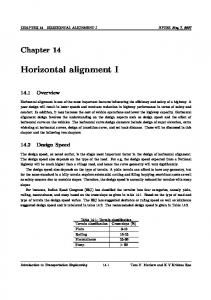
conditional propositions. All parts of the antecedent are evaluated simultaneously and resolved to a single number using the logical operators in Table 1, that is, AND, OR, and NOT. Fuzzy reasoning, known also as approximate reasoning, is the process of deriving conclusions from a set of IF-THEN fuzzy rules using an inference procedure. By fuzzy reasoning, the truth of the consequent is inferred from the degree of truth of the antecedent. The concept of fuzzy set theory, IF-THEN rules, and fuzzy reasoning together constitute a computing framework usually called fuzzy inference system (FIS). The structure of a fuzzy inference system consists of three major parts: a rule base that holds the fuzzy IFTHEN rules used in the inference process, a database that contains the membership functions that characterize the fuzzy sets, and a reasoning mechanism that performs the inference procedure and derives conclusions depending on a set of rules and facts. The fuzzy inference process thus consists of five steps including fuzzification, application of the fuzzy operators, fuzzy implication, fuzzy aggregation, and defuzzification, as schematically summarized in Figure 2. The function of the fuzzification is to determine the degree of membership to a crisp input in a fuzzy set. The fuzzy rule base is used to present the fuzzy relationship between inputoutput fuzzy variables. The output of the fuzzy rule base is determined based on the degree of membership specified by the fuzzifier. The defuzzification is used to convert outputs to the fuzzy rule base into crisp values. In recent years, fuzzy logic has been successfully applied in a variety of disciplines including engineering, computer vision, weather prediction, image processing, nuclear reactor control, control of biomedical processes, automatic tuning, and many other fields of research [39]. Little has however been done on the practical application of fuzzy logic and AHP, especially in intelligent transportation based decision making.
6
Advances in Civil Engineering
Input
Fuzzification
If-then rule base
Output
Defuzzification
Knowledge base (rule and function)
Membership function
Figure 2: A block diagram of generalized fuzzy system.
Decision making team
Create fuzzy pairwise comparison matrix of experts (̃J)
(transport engineers and planners)
Determining and standardizing the evaluation factors Check for consistency (CI) for the most likely value Structuring decision hierarchy Adjust decision weights
Adjust structure
No
CI < 10%?
Approve decision hierarchy
Yes
Yes
Calculate the fuzzy weights (WF kn = Wi × MF i )
Assigning criteria weights via AHP
Aggregate standardized individual criteria
No
Adjust factor weights No
Approve criteria weights
Fuzzy defuzzification
Yes
Constraint factor and GIS-LCP
Least cost path (LCP) finding
Decision making and validation (least cost highway bypass location and horizontal alignment)
Figure 3: Schematic framework of the proposed methodology for least cost bypass horizontal alignment selection based on fuzzy AHP with GIS-LCP analysis.
In fuzzy AHP (F-AHP), instead of single crisp value, a range of values are used. Out of this range, decision maker can pick up values as per his/her confidence and also can specify the associated attitude toward risk as optimistic, pessimistic, or moderate. To take care of the risk attitude, optimistic attitude takes the highest value of the range, pessimistic attitude takes the lowest value in the range, and moderate attitude takes the middle value of the uncertain range.
In related linear engineering structures (LES) studies, Nataraj [41] used AHP in pipeline route location, Moghaddam and Delavar [35] used GIS-based fuzzy logic in oil and gas pipeline location optimization in Iran, and Dell’Acqua [20] used fuzzy inference systems to optimize highway alignments in Italy. Notably, not much LES intelligent based studies have been reported on actual highway bypass location projects especially in developing countries.
Advances in Civil Engineering Level 1 (goal)
7
1 X1,0
2 X1,1
Level 2 3 Level 3 X1,1
Level 4 (evaluation alternative) k Xi,j
2 X3,1
2 X2,1 3 X1,3
3 X2,1
A1
3 X2,3
3 X3,3
A3
A2 The item does not have dependent children
Legend Level k Xi,j Child Parent
Figure 4: Hierarchical tree example for four-level structure [33]. The levels can be reduced to 3 or more than 4 depending on the project.
𝜇m
M1
V(M2 ≥ M1 )
M2
D
of comparison interval and proposed a methodology based on stochastic optimization to achieve global consistency, while Leung and Cao [48] discussed the consistency issue and proposed a concept of fuzzy consistency and tolerance deviation. Further, Yu [49] proposed goal programming to compute the fuzzy priority vectors and Arslan and Khisty [50] proposed a set of IF-THEN rules to select the cognitive comparisons made between each alternative. Wang et al. [51] presented a two-stage logarithmic goal programming method for generating weights from interval comparison matrices. On the application side, [52, 53] presented evaluation of services using F-AHP. These reviews demonstrate that fuzzy AHP approach has been considered to a large extent in theory and to a smaller extent in practical applications. This study builds on the interpretation of F-AHP by incorporating the decision maker’s attitude in the final decision making process as was originally proposed by [46, 54]. On the determination of the most suitable location and horizontal alignment from the F-AHP alternatives the theory of least cost path (LCP) is used in a GIS platform. The schematic framework of the modified F-AHP approach in this study is presented in Figure 3. In this study, decision makers (experts) are the transportation engineers and planners. A step-by-step summary of the F-AHP methodology is presented in the following six stages. Stage 1. Hierarchical organization of the attribute/indicator characteristics to be analyzed for the bypass horizontal alignment determination. Stage 2. Standardizing attribute or indicator characteristics using asymmetric and symmetric models.
l2
m2
l1
d u2
m1
u1 M
Figure 5: The comparison of two fuzzy numbers 𝑀1 and 𝑀2 and intersection between two TFNs [34].
2.3. Fuzzy Analytic Hierarchy Process (F-AHP). This study argues that for the analysis of physical phenomena in decision making, the subjective pairwise comparison is prone to vagueness type uncertainty as already stated and can only be best analyzed using fuzzy-based analyses. The first attempt in the integration of fuzzy-based technique with AHP appeared in [42] who compared fuzzy ratios described by TFNs and weight computed using logarithmic least squares method. Buckley [17] highlighted the shortcomings in their method and proposed a geometric mean to derive fuzzy weights and performance scores. Boender et al. [43] modified van Laarhoven and Pedrycz [42] normalization method by implementing a regression equation. Later Chang [34] introduced the use of the extent analysis method for the synthetic extent values of the pairwise comparisons. While Cheng [44] introduced the entropy concepts to calculate aggregate weights, Zhu et al. [45] improved on the extent analysis. Deng [46] presented a fuzzy-based approach for handling multicriteria analysis problems by incorporating the decision maker’s attitude toward risk. Lee et al. [47] introduced the concept
Stage 3. Weighting factors. Weighting the model criteria provides relative measures of the interaction and importance of each attribute/indicator (factors). The weights are obtained through a pairwise comparison analysis in an AHP approach in discussion with experts. The experts play an important role in the iterative adjustment of weights to improve the consistency ratio (CI). Stage 4. Deriving the weighted map layers of the criterion. The weighted criterion layers are generated using the function: WF𝑘𝑛 = 𝑊𝑖 ×MF𝑖 , where 𝑊𝑖 is the weight of the criteria factor from the pairwise comparison and MF𝑖 is the membership function for the criteria. Stage 5. Deriving the overall location suitability map layers. The suitability is calculated by combining the weighted criterion layers. This function sums the weighted fuzzy maps of the different factors’ proprieties to obtain suitability maps at the final level using the equation: 𝑅𝑖 = WF𝑘1 + WF𝑘2 + ⋅ ⋅ ⋅ + WF𝑘𝑛 , where 𝑅𝑖 is the overall rating score for the suitability of land and WF𝑘𝑛 is the weighted value for the different criterion. Stage 6. Most suitable route location determination. The overall suitability location map is obtained using the least cost path (LCP) comparison and determination through GIS analysis. At this stage, the constraint factor(s) are introduced.
Advances in Civil Engineering
Determined input criteria of factors
8
W0
W1 Fuzzy implication
W2 W3 W4
⊗ ⊗
Fuzzy aggregation
⊗
Deffuzification
Degree of suitability
⊗ ⊗
Fuzzy rule base based on AHP
Figure 6: Highway bypass factors in fuzzy inference system combined with AHP derived fuzzy rule (simplified from Figure 3 for purposes of implementation).
Elevation (EL) Slope (SP) Physical criteria
Soils (SW) Geology (GL) Drainage networks (DN)
Bypass horizontal alignment route determination
Land-use (LU) Socioeconomic criteria Road network (RN)
CBD and zoning map of Eldoret municipality Constraint Size and extent of case study area Goal
Objectives or dimension
Criteria or factors
Figure 7: Three-level hierarchical structure of the characteristics for the highway bypass location project.
2.3.1. Development of Decision Hierarchical Structures. Developing the hierarchical decision model consists of the decomposition of the “complex” decision problem into smaller manageable elements of different hierarchical tree/layers. An example four-level hierarchical tree is illustrated in Figure 4 [33]. The first layer of the hierarchy corresponds to the objective or goal, and the last layer corresponds to the evaluation alternatives (options), whereas the intermediate
levels correspond to criteria and subcriteria being considered in the project. In Figure 4, the nomenclature adopted for each item in 𝑘 , where 𝑖 is the order of the the hierarchical model is 𝑋𝑖,𝑗 child at the level/layer 𝑘 and 𝑗 is the parent of the child 2 [33]. For example, 𝑋1,1 shows the item is at level 𝑘 = 2, is the first child 𝑖 = 1, and its parent is 𝑗 = 1. Each child,
Advances in Civil Engineering —
9
Study area 35
.192285
35
237100
35
281915
Source and destination(s)
35326730
35371545
35
.192285
35
C
237100
35281915
35326730
35371545
C
0545886
0545886
0545886
0545886 CBD
0497279
0497279
0448883
0448883
A
0400047
0400047 B
35
.192285
BAC
35
237100
35
281915
35
326730
0497279
0448883
0448883
A
0400047
0400047
B
0361431 35
371545
35
N
Municipality boundary A104 highway
0497279
S 0 1 2
4 6 (km)
35
237100
35
281915
35
326730
0361431
35
371545
N
Source and destinations A Royalton C Maili-Nne B Cheptiret
E
W
.192285
E
W S 0 12
8
4 6 (km)
8
(b)
(a)
Figure 8: (a) Eldoret municipality boundary overlaid on the topographic map of the area. (b) Source and destination points on the current A104 highway passing through the CBD.
in the intermediate levels, is criterion and subcriterion that affect the corresponding parent and child, respectively. The apostrophe on any intermediate item (element, factor, 𝑘 subcriterion), 𝑋𝑖,𝑗 , indicates that the element does not have dependent children. The shaded items correspond to levels 2 2 3 3 3 and 3, that is, 𝑋3,1 , 𝑋1,3 , 𝑋2,3 , and 𝑋3,3 . 2.3.2. Development of Fuzzy Judgment Matrix Using AHP Pairwise Comparisons. The elements of a particular level are compared pairwise with a specific element of an upper level ̃ is generated using (Figure 4). A fuzzy judgment matrix (𝐽) fuzzy pairwise comparison index (𝑗̃𝑖𝑗 ). A relative importance (strength) of the pairwise comparison is assigned using a scale of 1–9 (Table 2) [6, 7], which are fuzzified to capture vagueness in perception and meaning as depicted in Table 3. For 𝑛 number of comparison items, the fuzzy judgment matrix 𝐽̃ is represented by 𝑗̃11 [𝑗̃ 21 𝐽=[ [⋅ [𝑗̃𝑛1
𝑗̃12 𝑗̃22 ⋅ 𝑗̃𝑛2
⋅⋅ ⋅⋅ ⋅ ⋅⋅
𝑗̃1𝑛 𝑗̃2𝑛 ] ]. ⋅ ] 𝑗̃𝑛𝑛 ]
For diagonal entries, that is, 𝑖 = 𝑗, 𝑗̃𝑖𝑗 = 1. The upper righthand triangle entries 𝑗̃𝑖𝑗 are comparison items that are defined by the decision maker, whereas lower left-hand triangle entries are derived by taking reciprocals; that is, 𝑗̃𝑗𝑖 = 1/𝑗̃𝑖𝑗 . 2.3.3. Calculation of Fuzzy Weights. Various techniques can be used to compute the final fuzzy weights, such as computation of the eigenvector, arithmetic mean, geometric mean, and so forth. Preliminary investigation carried out using these techniques showed no significant difference. Consequently, for ease of implementation, the geometric mean is adopted to estimate the weights. Fuzzy arithmetic operations (Table 4) are utilized over matrix 𝐽̃ to compute ̃ the the fuzzy weights. Following the previous example for 𝐽, ̃ ̃ geometric mean is computed for each row 𝐽𝑖 : given 𝐽 from (6), the corresponding fuzzy weights are computed as 1/𝑛 𝐽̃𝑖 = (𝑗̃𝑖1 ⊗ ⋅ ⋅ ⋅ ⊗ 𝑗̃𝑖𝑛 ) −1
(6)
̃𝑖 = 𝐽̃𝑖 ⊗ (𝐽̃1 ⊕ ⋅ ⋅ ⋅ ⊕ 𝐽̃𝑛 ) , 𝑤 ̃𝑖 is the fuzzy weight and 𝑖 = 1 to 𝑛. where 𝑤
(7)
10
Advances in Civil Engineering
DEM 35
.192285
35
237100
35
281915
Slope 35371545
35326730
35
.192285
35
237100
35
281915
35326730
35371545
0545886
0545886
0545886
0545886
0497279
0497279
0497279
0497279
0448883
0448883
0448883
0448883
0400047
0400047
0400047
0400047
0361431
0361431 35
.192285
35
237100
35
281915
35
326730
Elevations (m) 1,989–2,032 2,032.000001–2,059 2,059.000001–2,082 2,082.000001–2,101 2,101.000001–2,118 2,118.000001–2,135 2,135.000001–2,152 2,152.000001–2,170 2,170.000001–2,189 2,189.000001–2,229
35
371545
35.192285
N E
W S 0 1 2
4 6 (km)
8
35237100
35281915
35326730
Slope (deg) 0–1.671503793 1.671503794–3.494962475 3.494962476–5.166466268 5.166466269–6.83797006 6.837970061–8.813383633 8.813383634–11.39661677 11.39661678–14.89157924 14.89157925–21.27368463 21.27368464–38.74849701
35371545 N E
W S 0 1 2
4 6 (km)
8
(b)
(a)
Figure 9: (a) DEM of the study area from 30 m × 30 m ASTER Global DEM. (b) Slope map of the study area derived from the DEM.
Table 4: Definition of fuzzy numbers and their scale as used for making pairwise comparisons. Relative importance 1̃
a
Fuzzy scale
b
Definition
Explanation
(1, 1, 1)
Equal importance
̃3
(3 − Δ𝑐 , 3, 3 + Δ)
Weak importance
5̃
(5 − Δ, 5, 5 + Δ)
Essential or strong importance
7̃
(7 − Δ, 7, 7 + Δ)
Demonstrated importance
9̃
(8, 9, 9)
Extreme importance
Two activities contribute equally to objective Experience and judgment slightly favour one activity over another Experience and judgment strongly favor one activity over another One activity is strongly favoured and demonstrated in practice The evidence favouring one activity over another is of highest possible order of affirmation
(𝑥 − Δ, 𝑥, 𝑥 + Δ)
Intermediate values between two adjacent judgments
2̃, 4̃, 6̃, 8̃ 1/𝑥̃ 1/9̃ a c
When compromise is needed
(1/(𝑥 + Δ), 1/𝑥, 1/(𝑥 − Δ) (1/9, 1/9, 1/8)
The intensity of importance definition is in accordance with the description proposed by [6, 7]; b minimum, most likely, and maximum values. Δ is a fuzzification factor.
Advances in Civil Engineering
11
Land-use 35
.192285
35
237100
35
281915
35
Zoning map 326730
35
371545
35
0545886
0545886
0497279
0497279
0448883
0448883
0400047
0400047
35.192285
35237100
35281915
35326730
35371545
Built-up areas Nonurban area
S 0 1 2
4 6 (km)
35281915
35326730 0594511
0545886
0545886
0497279
0497279
0448883
0448883
35237100
35281915
35326730
N Zoning map for Eldoret town Educational and cultural E W Commercial S Administration and public utilities Agricultural 0 0.5 1 2 3 Industrial (km) Residential Transport
E
W
35
237100
0594511
35.192285
N
Land-use
.192285
8
(a)
4
(b)
Figure 10: Land-use and land-cover depicting (a) built-up urban and nonurban areas classified from Landsat ETM+ and (b) zoning map of the Eldoret town municipality.
2.3.4. Establishment of Hierarchical Layer Sequencing: Weighing and Fuzzy AHP Scoring. The local priorities at each level are aggregated to obtain final preferences of the alternative. This computation can be carried out from the evaluation alternatives (bottom level) to the top level (goal or objective) or vice versa depending on the knowledge and expertise of the decision makers and on the number of objectives being considered. As depicted in Figure 4, each of the three alternatives, 𝐴 𝑖 , 𝑖 = 1, 2, 3, is aggregated through level 3, level 2, and finally to level 1 (goal). Therefore, following Figure 4 at ̃𝑘 ) are each level of 𝑘, the fuzzy global preference weights (𝐺 computed as ̃𝐾−1 ̃𝑘 = 𝑤 ̃𝑘 ⋅ 𝐺 𝐺 ̃1 = 𝑤 ̃1 ; 𝐺
̃2 = 𝑤 ̃1 ; ̃1 ⋅ 𝐺 𝐺
̃3 = 𝑤 ̃2 ; ̃3 ⋅ 𝐺 𝐺
(8)
̃4 = 𝑤 ̃3 . ̃4 ⋅ 𝐺 𝐺
The final fuzzy AHP score (𝐹̃𝐴 𝑖 ), for each alternative 𝐴 𝑖 , is obtained by carrying out fuzzy arithmetic sum over each global preference weights: 𝑛
̃𝑘 , 𝐹̃𝐴 𝑖 = ∑ 𝐺 𝑘−1
for each study criteria or alternative (𝐴 𝑖 ).
(9)
2.3.5. Ordering Result Alternatives Using Fuzzy Ranking Method through Fuzzy Defuzzification. Fuzzy defuzzification methods can be used for ranking fuzzy numbers. Defuzzification entails converting the final fuzzy AHP score 𝐹̃𝐴 𝑖 into a crisp value. Once the final fuzzy AHP score (𝐹̃𝐴 𝑖 ) of each alternative is defuzzified, the crisp numbers are compared and ranked accordingly. Various techniques are used for defuzzification; however, each technique extracts different levels of information from the fuzzy numbers and consequently may give different ranking orders [55]. This implies that an alternative ranked the best may be ranked differently upon changing the defuzzification technique, and is commonly called rank reversal, which is a common concern in AHP analysis [8]. This problem is further aggravated with the fuzzy outputs and the use of different defuzzification techniques. This induces a dilemma on the decision maker’s part for the selection of an alternative [56]. This uncertainty is taken through decision maker’s risk attitude analysis, discussed in Section 2.3.6 below. 2.3.6. Incorporating Risk Attitude in Decision Making. The final decision making based on fuzzy output of an alternative (𝐴 𝑖 ) induces undue burden on the decision maker since there is an infinite solution space. The final ranking can
12
Advances in Civil Engineering And finally,
Road networks 35.192285 35237100 35281915 35326730 35371545
0545886
B10/1
𝑤 = 𝜆𝑤3𝛼 + (1 − 𝜆) 𝑤1𝛼 .
C626/1
0545886 CBD
0
497279
C646
C581
0497279
C648
B11/1 A104
0448883
2.4. F-AHP Implementation. Let 𝑋 = {𝑥1 , 𝑥2 , . . . , 𝑥𝑛 } and 𝑍 = {𝑧1 , 𝑧2 , . . . , 𝑧𝑚 } be an object and goal sets, respectively. According to the extent analysis technique, for each objective function, extent analysis is carried out with respect to each goal set. Hence, 𝑚 extent analysis values for every object set are given by
0448883
0400047
0400047
0361431
0361431
1 2 𝑚 , 𝑀𝑔𝑖 , . . . , 𝑀𝑔𝑖 ; 𝑀𝑔𝑖
FS𝑖 =
E
W S 0 1 2
4 6 (km)
8
Figure 11: Digitized and classified major road networks within the study area.
be undertaken by incorporating the decision maker’s risk tolerance (attitude) and confidence over the evaluation, which is more subjective. The 𝛼-cut concept described earlier represents the decision maker’s degree of confidence in the fuzzy assessment (i.e., 𝛼 = 0 entails lack of confidence over the fuzzy assessment and hence utilizes the full range of uncertainty, whereas the higher value of 𝛼 represents a more confident decision maker and reaches maximum when the value approaches the “most likely” value). For any given 𝛼-cut on a TFN, the notation used is (𝑎𝛼 , 𝑏, 𝑐𝛼 ). Further, given the desired confidence over the data, the risk attitude has a significant effect on the defuzzified value using the decision maker’s risk attitude index, 𝜆 RI [46]. In order to avoid the contradiction of subjective judgments following defuzzification, the consistency should be checked by already discussed CI and CR above. 2.3.7. Defuzzification of the Fuzzy Weighting. To prioritize the risk factors in decision making, the fuzzy weighting needs to be compared and ranked. To facilitate the pairwise comparison process and to avoid the complex and unreliable ̃ ⊗ 𝐵̃ = process of comparing fuzzy weighing, the 𝛼-cut (𝐴 ̃ 𝐵̃ = (𝑎1 𝑏1 , 𝑎2 𝑏2 , 𝑎3 𝑏3 )) and risk index (𝜆) expressed as 𝐴/ (𝑎1 /𝑏3 , 𝑎2 /𝑏2 , 𝑎3 /𝑏1 ) are used to defuzzificate the fuzzy weighing and get a crisp weighing of each risk factor; that is, 𝑤1𝛼 = 𝑤1 + 𝛼 (𝑤2 − 𝑤1 ) 𝑤3𝛼 = 𝑤3 − 𝛼 (𝑤3 − 𝑤2 ) .
(10)
(12)
𝑗
N C581 C626/1 C646
𝑖 = 1, 2, . . . , 𝑛,
where 𝑀𝑔𝑖 (𝑗 = 1, 2, . . . , 𝑚) are the TFNs. The value of fuzzy synthetic FS𝑖 extent with respect to the 𝑖th object is defined by
35.192285 35237100 35281915 35326730 35371545
Road classification B11/1 C648 A104 B10/1
(11)
𝑚
𝑗 ∑ 𝑀𝑔𝑖 𝑗=1
𝑛
𝑚
−1
𝑗 ⊗ [∑ ∑ 𝑀𝑔𝑖 ] . [𝑖=1 𝑗=1 ]
(13)
For calculation of F-AHP priority vectors, fuzzy pairwise comparison matrix 𝐴 = (𝑎𝑖𝑗 )𝑚∗𝑛 is considered, in which 𝑎𝑖𝑗 = (𝑟𝑖𝑗 , 𝑠𝑖𝑗 , 𝑡𝑖𝑗 ), where 𝑟, 𝑠, and 𝑡 are defined as the lower, modal, and upper values of the triangular fuzzy number (𝑀), 𝑗 respectively. In this the TFNs (∑𝑚 𝑗=1 𝑀𝑔𝑖 ) can be accomplished by fuzzy addition operation for the 𝑚 extent analysis values in such a way that 𝑚
𝑗
𝑚
𝑚
𝑚
𝑗=1
𝑗=1
𝑗=1
∑ 𝑀𝑔𝑖 = ( ∑ 𝑟𝑖𝑗 ∑ 𝑠𝑖𝑗 ∑ 𝑡𝑖𝑗 ) ;
𝑗=1
𝑛
𝑖 = 1, 2, . . . , 𝑛,
−1
𝑚
[∑ ∑ 𝑀𝑗 ] 𝑔𝑖 𝑖=1 𝑗=1
(14)
]
[
=(
∑𝑛𝑖=1
1 1 1 , 𝑛 , 𝑛 ). 𝑚 𝑚 ∑𝑗=1 𝑡𝑖𝑗 ∑𝑖=1 ∑𝑗=1 𝑠𝑖𝑗 ∑𝑖=1 ∑𝑚 𝑗=1 𝑟𝑖𝑗
Subsequently, the degree of possibility of 𝑀2 = (𝑟2 , 𝑠2 , 𝑡2 ) ≥ 𝑀1 = (𝑟1 , 𝑠1 , 𝑡1 ) can be expressed as 𝑉 (𝑀2 ≥ 𝑀1 ) = sup [min (𝜇𝑀1 (𝑥) , 𝜇𝑀2 (𝑦))] 𝑥≥𝑦
𝑉 (𝑀2 ≥ 𝑀1 ) = ℎ𝑔𝑡 (𝑀1 ∩ 𝑀2 ) = 𝜇𝑀2 (𝑑) 1, if 𝑠2 ≥ 𝑠1 { { {0, if 𝑟1 ≥ 𝑡2 ={ 𝑟 ≥ 𝑡 { 1 1 { , otherwise, { (𝑠2 ≥ 𝑡2 ) − (𝑠1 ≥ 𝑟1 ) (15) where 𝑑 is the ordinate of the highest intersection point of the triangular fuzzy network between 𝜇𝑀1 and 𝜇𝑀2 as demonstrated in Figure 5. Furthermore, an extent of possibility for
Advances in Civil Engineering
13
Geological structure 35
.192285
35
237100
35281915
35326730
Soil types 35371545
35
.192285
35
237100
35
281915
35326730
35371545
0545886
0545886
0545886
0545886
0497279
0497279
0497279
0497279
0448883
0448883
0448883
0448883
0400047
0400047
0400047
0400047
0361431
0361431
35.192285
35237100
35281915
35326730
Geology Aphanitic phonolite Porphyritic phonolite
35371545
35.192285
E S
0 1 2
4 6 (km)
35281915
35326730
Soil types Loamy clayey Loamy Clayey
N W
35237100
35371545 N
S
8
0 1 2
(a)
E
W
4 6 (km)
8
(b)
Figure 12: (a) Geological structure of the study area described by aphanitic and porphyritic structures. (b) Types and distribution of soil cover within the study area.
a convex fuzzy number to be larger than 𝑘 convex fuzzy number 𝑀𝑖 for 𝑖 = 1, 2, . . . , 𝑘 can be calculated according to 𝑉 (𝑀 ≥ 𝑀1 , 𝑀2 , . . . , 𝑀𝑘 ) = 𝑉 (𝑀 ≥ 𝑀1 ) , (𝑀 ≥ 𝑀2 ) , . . . , (𝑀 ≥ 𝑀𝑘 ) = min 𝑉 (𝑀 ≥ 𝑀𝑖 )
(16)
The F-AHP implementation with extent analysis can summarily be represented by the following steps. These steps are illustrated in Figure 6, where 𝑊𝑖 is the criteria weight. Step 1. Acquisition of normal (crisp) pairwise comparison matrices (PCM). Step 2. Fuzzifying the crisp PCM to fuzzy PCM.
for (𝑖 = 1, 2, . . . , 𝑘) .
Step 3. Calculation of performance ratings using fuzzy extent analysis.
Assume that
Step 4. Weightage multiplication from hierarchy.
𝑑 (𝐴 𝑖 ) = min 𝑉 (FS𝑖 ≥ FS𝑘 )
(17)
for (𝑘 = 1, 2, . . . , 𝑛) , 𝑘 ≠ 1,
then the value of weight vector (𝑊 ) for 𝐻𝑖 = 1, 2, . . . , 𝑛, for 𝑛 number of elements, can be expressed as 𝑇
𝑊 = (𝑑 (𝐻1 ) , 𝑑 (𝐻2 ) , . . . , 𝑑 (𝐻𝑛 )) .
𝑇
Step 6. Embedding attitude of the decision maker through lambda function. Step 7. Normalizing the effect table.
(18)
After normalization of (18), a nonfuzzy number (𝑊) is represented as given below: 𝑊 = (𝑑 (𝐻1 ) , 𝑑 (𝐻2 ) , . . . , 𝑑 (𝐻𝑛 )) .
Step 5. Embedding uncertainty of decision maker (confidence) through alpha-cut analysis.
(19)
Step 8. Positive and negative ideal similarity vector identification. Step 9. Similarity measurement using vector matching function. Step 10. Final performance index measurement.
14
Advances in Civil Engineering Stream networks 35
.192285
35
237100
35281915
35326730
35371545
0594511
0594511
0545886
0545886 Sosiani river
0497279
0497279
0448883
0448883 Kipkaren river
0400047
0400047 Nureri river
0361431
0361431 35.192285
35237100
35281915
35326730
35371545 N
0 1 2
4 6 (km)
8
E
W S
Figure 13: Drainage networks showing the main rivers: Sosiani, Kipkaren, and Nureri.
The selection of suitable highway bypass comprises of consideration of several physical environmental and engineering factors or criteria. In this study, the following seven data factors were determined: elevation from digital elevation model (DEM)-EL; slope computed from the DEM (SP); land-use and land-cover (LU); existing major road networks (RN); geology (GL); soils types (SW); and stream or drainage networks (DN). These criteria are supposed to take care of topography, environmental, physical, and socioeconomic factors (Figure 7). In Figure 7, a three-level hierarchical tree structure is adopted to take care of the two objectives or dimensions: physical and socioeconomic considerations. A weightless constraint factor was introduced in the criteria hierarchy to ensure that the proposed bypass does not pass through the central business district (CBD) of Eldoret town, from which the traffic congestion is to be eased, and is not far away from the municipal boundaries or extents. Another salient constraint is the maximum length of the bypass that could be financed. This factor was incorporated indirectly by defining the extent of the study area.
3. Case Study and Data Sources 3.1. Case Study Problem. The rapid population and economic growth in Eldoret town municipality (Figure 8(a)) have resulted in continuous traffic congestion in the central
business district (CBD). This situation is aggregated by the fact that the town serves as a modal point for the transit of heavy goods to Uganda and the neighboring countries from the port of Mombasa. To ease the traffic congestion, the Kenya National Highways Authority (KeNHA) has decided to construct a 45 m multilane international trunk (class A) bypass. One of problems with the proposed project is that there is no reserved highway bypass corridor. Thus KeNHA has to come up with an optimal route and compensate land owners whose properties lie in the proposed route. Figure 8(a) shows the extent of the Eldoret municipality overlaid on the topographic map of the area. Figure 8(b) shows the current A104 highway and the proposed modal points of the new bypass, with origin being at Royalton (A) and destination at Maili-Nne (C). Point B (Cheptiret) is used in this study to validate the reliability of the determined optimal bypass by assuming the bypass starts from B and is constrained to pass through A and C. 3.2. Data Sources: Evaluation Criteria. This section presents the datasets (criteria) (Figure 7), as used in the determination of the location of the proposed highway bypass. 3.2.1. Digital Elevation Model (DEM) and Slope. While distance is the most fundamental cost of moving through a space, humans select routes based on more than just distance. A related contributing criterion to distance is the slope of the surface, since flatter terrain allows for more direct, faster, and easier travel. A raw numerical value of the slope clearly cannot be equated with the cost of overcoming that slope since many different quantifying schemes exist. It may seem reasonable to say that the cost of overcoming a zero degree slope is zero; thus the slopes should be as minimum possible. Also, downhill speeds, while relatively faster at shallow slopes than their uphill equivalents, are relatively slower at higher slopes. Moving downhill on steep slopes is more dangerous than uphill travel, requires more caution, and typically results in faster speeds. Terrain elevation data should be represented as continuous phenomena rather than discrete objects in order to fully model the land surface. Digital elevation model (DEM) is a digital representation of the continuous elevation variation of the land surface. Elevation data plays an important role in determining which areas may be suitable according to the technical requirements in optimum route design. For the study area, ASTER Global DEM at 30 m spatial resolution was used (Figure 9(a)). The corresponding slope map is represented in Figure 9(b). From Figure 9, it is observed that the elevation varied from a minimum of 1 989 m to a maximum of 2 229 m, and the corresponding slope ranges from 0∘ to 38∘ . 3.2.2. Land-Use and Land-Cover. Information on land-use and land-cover data is necessary in specifying the impacts of the suggested highway on the surrounding environment, where the highway will pass, and also in determining the degree of compensation for any acquired land. For this study, the land-use and land-cover, respectively, comprised of
Advances in Civil Engineering
15
Linear elevation map 35.192285
35237100
35281915
35326730
Linear slope map 35371545
35
.192285
35
237100
35281915
35326730
35371545
0545886
0545886
0545886
0545886
0497279
0497279
0497279
0497279
0448883
0448883
0448883
0448883
0400047
0400047
0400047
0400047
35.192285
35237100
35281915
35326730
35371545
N 0.5–0.55 E W 0.55-0.6 S 0.6–0.65 0.65–0.7 0.7–0.75 0 1 2 4 6 0.75–0.8 (km) 0.8–0.85 0.85–0.9 0.9–0.95 0.95–1
Membership 0–0.05 0.05–0.1 0.100000001–0.15 0.15–0.2 0.2–0.25 0.25–0.3 0.3–0.35 0.35–0.4 0.4–0.45 0.45–0.5
35.192285
8
(a)
35237100
35281915
Membership 0–0.05 0.05–0.1 0.100000001–0.15 0.15–0.2 0.2–0.25 0.25–0.3 0.3–0.35 0.35–0.4 0.4–0.45 0.45–0.5
35326730
0.5–0.55 0.55-0.6 0.6–0.65 0.65–0.7 0.7–0.75 0.75–0.8 0.8–0.85 0.85–0.9 0.9–0.95 0.95–1
35371545 N E
W S 0 1 2
4 6 (km)
8
(b)
Figure 14: Standardized linear fuzzy maps for (a) elevation and (b) slope for the study area.
the built-up (urban) and nonurban areas, and were derived through unsupervised classification of Landsat 8 ETM+ data with results in Figure 10(a). The built-up area was segmented using the municipality zone map (Figure 10(b)). The zone map comprised of 7 polygons of land-use as educational and recreational, commercial, administration and public utilities, agricultural, industrial, residential, and transport zones. In the implementation, the zoning map (except for the agricultural areas) is treated as highly restricted area for the bypass route and thus is expressed as “no-data” map. By applying Boolean logic, the study area is constrained into two classes of suitable (value 1) and unsuitable (value 0). The mathematical formulation in area selection by using constraint criteria is expressed as SI = ∏𝐾 𝑗=1 𝑏𝑗 , where SI = total suitability index value (0 or 1); 𝑏𝑗 = suitability index value for each constraint criterion (0 or 1); and 𝐾 = total number of constraint criteria [57]. 3.2.3. Existing Major Road Network. Existing road network is an important evaluation factor since the distances to the existing major roads depict the connections to and from
the proposed bypass. The bypass should not cross or pass too near the existing major roads in order to minimize the construction of roundabouts and other related road furniture. Figure 11 shows the digitized and classified major road networks within the study area. The bypass should originate from and reconnect to the current A104 highway. 3.2.4. Geological Structure and Soils Types. The geological structure influences the type and property of soils within a given area and thus influences the flexible pavement foundation. The project area is characterized by two main geological formations: aphanitic and porphyritic geological structures (Figure 12(a)). Figure 12(b) shows the distribution and types of soils as loamy, clayey, and loamy clayey, with the latter two dominating the study scene. 3.2.5. Drainage Networks. Drainage networks depict the distribution of major rivers within the study area. This is an essential cost-factor as it influences the cost of constructing bridges. By determining the hydrologic flow accumulation from the DEM, the three main drainage networks (rivers) within the study area were derived (Figure 13). Minor streams
16
Advances in Civil Engineering Euclidian distances to roads 35.192285
35237100
35281915
35326730
Linear roads map 35371545
35
.192285
35
237100
35281915
35326730
35371545
0545886
0545886
0545886
0545886
0497279
0497279
0497279
0497279
0448883
0448883
0448883
0448883
0400047
0400047
0400047
0400047
35.192285
35237100
35281915
Euclidian distances to roads (m) 0–362 363–950 951–1555 1556–2189 2190–2851 2852–3571 3572–4349 4350–5184 5185–6077 6078–7344
35326730
35371545
35.192285
N E
W S 0 1 2
4 6 (km)
8
(a)
35237100
35281915
Membership 0–0.05 0.05–0.1 0.100000001–0.15 0.15–0.2 0.2–0.25 0.25–0.3 0.3–0.35 0.35–0.4 0.4–0.45 0.45–0.5
35326730
0.5–0.55 0.55-0.6 0.6–0.65 0.65–0.7 0.7–0.75 0.75–0.8 0.8–0.85 0.85–0.9 0.9–0.95 0.95–1
35371545 N E
W S 0 1 2
4 6 (km)
8
(b)
Figure 15: (a) Euclidian distances to roads map and (b) corresponding standardized fuzzy membership.
and drainage channels were ignored since culverts can be erected instead of bridges. 3.3. Conditions for Highway Bypass Horizontal Alignment Location. The route cost can be analyzed under two main cost headlines: expropriation and construction costs. Highway bypass route determination should be located and designed with consideration of optimum time, cost, and productivity, whereby optimum cost is the most significant factor. The factors which affect the route’s construction cost are geology, soil, topography, land-use, and existing road network information. The factors that cause high or low expropriation cost by affecting the real estate value are topography and land-use. To locate the optimal horizontal alignment of the proposed bypass, the following data conditions were considered. (i) The selected route should be the least cost alternative. To achieve this, the following factors were further taken into consideration. (ii) The elevation variations through the route should be kept as minimum as possible. The elevations for the study area ranged from 1 999 m to 2 229 m (Figure 9(a)). For the desired bypass length of less
than 20 km, elevations of between 2 005 m and 2 208 m were recommended as suitable. (iii) The slopes should also be kept as minimum as possible, with suitable slope being between 0∘ and 25∘ . The slope for the study area had a maximum of 38∘ ; thus slopes of up to 25∘ were considered suitable. (iv) The highway bypass route should not pass near existing major roads for the purposes of decongesting the CBD. A buffer distance of up to 1 343 m was chosen from the center of the CBD to cater for this condition. (v) The route should not pass within urban built-up areas in order to reduce the property damage and compensation costs. (vi) The route should not pass over streams and rivers to avoid construction of bridges and possible road destructions caused by overflows in event of flooding. A buffer distance of 183 m from the delineated major rivers was chosen for this study case. (vii) The geology and soil underlying the route should be suitable for flexible pavement foundation stability.
Advances in Civil Engineering
17
Euclidian distances to streams 35
.192285
35
237100
35281915
35326730
Linear streams map 35371545
35.192285
35237100
35281915
35326730
35371545
0545886
0545886
0545886
0545886
0497279
0497279
0497279
0497279
0448883
0448883
0448883
0448883
0400047
0400047
0400047
0400047
35.192285
35237100
35281915
Euclidian distances to streams (m) 0–632 633–1290 1291–2004 2005–2527 2528–3080 3081–3633 3634–4186 4187–4765 4766–5450 5451–6714
35326730
35371545
35.192285
N E
W S 0 1 2
4 6 (km)
(a)
8
35237100
35281915
Membership 0–0.05 0.05–0.1 0.100000001–0.15 0.15–0.2 0.2–0.25 0.25–0.3 0.3–0.35 0.35–0.4 0.4–0.45 0.45–0.5
35326730
35371545
N 0.5–0.55 E W 0.55-0.6 0.6–0.65 S 0.65–0.7 0.7–0.75 0 1 2 4 6 0.75–0.8 (km) 0.8–0.85 0.85–0.9 0.9–0.95 0.95–1
8
(b)
Figure 16: (a) Distance to drainage networks and (b) corresponding linear membership map for the drainage networks.
4. Results, Analysis, and Discussions This section presents the case study results, analyses, and discussions in the following steps in the preparation of the study datasets (factors). (i) Rasterization and reclassification of the criteria layers according to the evaluation options and fuzzy membership in order to create standardized and weighted attributes. (ii) Creation of thematic cost surface maps from the standardized and weighted hierarchical attributes. (iii) Generation of accumulated cost surface distances and backlink datasets as suitability map layers. (iv) Determining the F-AHP least cost bypass using the cost distance and backlink information in a GIS optimal path finding system. Rasterization is carried out to create raster data models, which are more suitable in the analysis of movements from cell-to-cell, rather than through an infinite directional space as in vector data models. As part of standardization, the raster datasets were resampled to 30 m × 30 m spatial resolution.
4.1. Rasterization and Reclassification of Decision Criteria. The rasterized datasets were classified into Euclidean distances to create the distance maps, which were reclassified into uniform data, based on the highway alignment conditions as set out in Section 3.3. The reclassified uniform data are converted to cost surface maps. For the point and linear-based criteria, linear cost-surfaces are generated, and for the polygonal-based features, free function cost-surface maps are created. The results are directed graph models for the movements through space in the evaluation factors, with standardization ranging from a minimum of 0 to a maximum of 1. 4.1.1. Linear Map for Elevation. For the elevation data, a negative elevation function was adopted where elevation of 2208 m was assigned a value one (1), while the least elevation of 2005 m a value zero. The reclassified elevation map is shown in Figure 14(a). The reclassified linear elevation map shows that most parts were suitably elevated for locating the bypass. Similarly for the slope map, slope of 0∘ was assigned a value one (1) which is most desirable and slope of 25∘ a value zero which is least desirable. The slope linear map in
18
Advances in Civil Engineering Fuzzy soil map
Fuzzy geology map 35.192285
35237100
35281915
35326730
35.192285
35371545
35237100
35281915
35326730
35371545
0545886
0545886
0497279
0497279
0497279
0448883
0448883
0448883
0448883
0400047
0400047
0400047
0400047
0361431
0361431
0545886
0545886
0497279
35.192285
35237100
35281915
Membership 0.5 0.5–0.699999988
35326730
35.192285
35371545
E S
0 1 2
4 6 (km)
35281915
35326730
Membership 0.100000002 0.100000002–0.498431361 0.498431361–0.899999976
N W
35237100
8
(a)
35371545 N E
W S 0 1 2
4 6 (km)
8
(b)
Figure 17: Free function maps for (a) geological structure and (b) soil types within the study area.
Figure 14(b) also indicates that most of the area is suitable for route location, as evidenced by the fuzzy membership values ranging between 0.75 and 1. 4.1.2. Road Networks: Euclidean Distance and Linear Maps. The distance to road map was reclassified using the fuzzy linear function, where distances close to the roads were assigned a value zero and those farthest away a value 1. Figure 15(a) shows the road Euclidean distances, and Figure 15(b) represents the fuzzy memberships for the distances. 4.1.3. Drainage Networks: Distance and Linear Maps. Through fuzzy reclassification, a positive drainage function was adopted where a distance of 183 m was assigned a value one (1), while lesser distances were assigned a value of zero (Figure 16). The results depict the fact that distances farthest from the main rivers were considered as the most suitable for locating the proposed bypass. 4.1.4. Free Functions for Geology and Soils. A value of 0.7 was assigned to the upper phonolite rock type and 0.5 to the lower phonolite rock classes, with the free function-based geologic reclassification results shown in Figure 17(a). These results imply that most of the area’s geological structure is
stable enough for the construction of the proposed flexible pavement. For the soils reclassification, a value of 0.9 was assigned to the loamy soil, 0.5 to loamy clay, and 0.1 to clayey soil. The soil reclassification results are presented in Figure 17(b). The results imply that most of the soil was fairly suitable for road bypass location as evidenced by the fuzzy value of above 0.5, with some sections requiring stabilization, that is, those that have fuzzy values of 0.1 (clay soils). 4.1.5. Free Function for Land-Use. In the free function reclassification of land-use, a value of 0.8 was assigned to nonurban areas and 0.1 to built-up areas resulting in Figure 18. As noted earlier, the zoning map is used to delineate the municipality boundary and to act as a no-data constraint criteria. 4.2. Weighting of Decision Factors. Following the decision judgment matrix, the CI is computed. The maximum eigenvalue evaluated was determined as (𝜆 max = 3.086). Thus, for a hierarchical level of 𝑛 = 3, the CI from (3) was deter-mined as (CI = 0.043), and the corresponding random index (RI) is obtained as 0.52. Finally, the consistency ratio (CR) is determined as equal to 8%, which is below the 10% threshold and hence the judgment matrix is acceptable. Using the geometric mean, as proposed for this study, the fuzzy weights are computed.
Advances in Civil Engineering
19
Fuzzy land-use map 35
.192285
35
237100
35
281915
35
326730
35
371545
0545886
0545886
0497279
0497279
0448883
0448883
0400047
0400047
0361431
0361431 35.192285 35237100 35281915 35326730 35371545
Membership Built-up areas Nonurban area
N E
W S 0 1 2
4 6 (km)
8
Figure 18: Free function for land-use in the study area.
First the pairwise comparison matrix is generated for the equally contributing physical subcriteria and socioeconomic subcriteria, as determined by the decision experts. For the case study, the two objectives (Figure 7) were interrelated and equally contributed in weight to the cost of locating the bypass. After subcriteria (factors) accounting in each of the two objective groups, the final weight is computed via multiplying obtained subcriteria weight by the related criteria weight in the upper level as discussed in the methodology. The results of the fuzzy weight determinations are presented in Table 5. From the results in Table 5, the socioeconomic criteria (land-use and road networks) had the highest significance among the decision making factors and are therefore considered to be the most costly in evaluating the viability of the project. 4.3. Generation of the Cost Surface Maps. Once a directed graph model for the movement through space is constructed (Section 4.1), the cost of movement through the surface is then determined according to the weights (Section 4.2). The costs are a representation of the combination of the factors that affect travel across a surface. Through fuzzy overlay, the suitability of the area or cell to travel through, or how much it costs to travel through a cell, is determined. For the point and linear criteria, the fuzzy
algebraic sum (𝜇Combination = 1 − ∏𝑛𝑖=1 (1 − 𝜇𝑖 )) is used to combine the linear themes, with the results in Figure 19(a). As depicted in Table 1, the fuzzy gamma is an algebraic product of fuzzy product (𝜇Combination = ∏𝑛𝑖=1 𝜇𝑖 ) and fuzzy sum operation, such that fuzzy gamma is computed as 𝜇Combination = (Fuzzy Sum)𝛿 ∗ (Fuzzy Product)1−𝛿 , where 𝜇𝑖 denotes the fuzzy weight of the 𝑖th factor, 𝜇Combination is the unit value in the output map, and the value of fuzzy gamma is determined between a min of 0 and max of 1. The correct value of fuzzy gamma generates an output map showing adoption between decreasing and increasing trend in the sum and product fuzzy operations. The criteria fuzzy sum map results show that most of the area is suitable for bypass location, as evidenced by fuzzy membership values ranging from 0.8 to 1. In combination with the free function datasets, fuzzy gamma (fuzzy 𝛾) results with an optimal value of 0.7 were overlaid with the sum map from the algebraic sum and the categorical data of soil, geology, and land-use to create the composite gamma costmap (Figure 19(b)). The result in Figure 19(b) also shows that most of the area within the study area is suitable in locating the bypass, that is, fuzzy membership values ranging from 0.65 to 0.85. To impose the constraint factor (“no-data” map) on the composite fuzzy gamma results, the fuzzy algebraic product is used to obtain the ultimate cost surface map. The fuzzy product ensures that the CBD area has no-data value so that in the LCP modelling, the highway does not pass through the CBD. The result of the final cost surface map is presented in Figure 20, with the CBD areas having the least or zero fuzzy membership for the bypass location. The cost surface map shows the region has different surface friction levels (expressed in fuzzy numbers), from which the most optimal or least cost route can be extracted. 4.4. Accumulated Cost Surface Distance and Least Cost Path Analysis. Finding a minimum path over a surface partitioned into regions of different frictions to movement has two aspects: (i) creation of an accumulated cost surface from a cost surface (where the frictions are stored); and (ii) tracing a minimum cost on the accumulated cost surface from a source point to a destination. A cumulative cost surface creates a new surface by assigning each cell a number that indicates the general least cost direction to the destination (ending) point. This direction surface is used to draw the LCP from the source node to the destination node. There are three main network problem models that are related to the ways that weights or resistances are assigned to each of the network links, namely, isotropic, partially anisotropic, and fully anisotropic [58]. In the full anisotropic network model, costs of passage are really anisotropic, as depicted in Figure 21. The cost of passage depends on location and direction, but there is one prevailing direction for the whole surface (e.g., it is easier to go left and up). In this type of problem, costs are variable over the surface and are direction dependent; however, the direction dependency is not in prevailing direction and is also variable over the surface [59].
20
Advances in Civil Engineering Gamma map
Sum map 35.192285
35237100
35281915
35326730
35.192285
35371545
35237100
35281915
35326730
35371545
0545886
0545886
0545886
0545886
0497279
0497279
0497279
0497279
0448883
0448883
0448883
0448883
0400047
0400047
0400047
0400047
0361431
0361431
0361431
0361431
35.192285
35237100
35281915
35326730
35.192285
35371545 N
Membership 0.433016807–0.45 0.45–0.5 0.5–0.55 0.55-0.6 0.6–0.65 0.65–0.7
0.7–0.75 0.75–0.8 0.8–0.85 0.85–0.9 0.9–0.95 0.95–1
E
W S 0 1 2
4 6 (km)
8
(a)
35237100
Membership 0.366721273–0.4 0.4–0.45 0.45–0.5 0.5–0.55 0.55-0.6
35281915
35326730
35371545 N
0.6–0.65 0.65–0.7 0.7–0.75 0.75–0.8 0.8–0.85
E
W S 0 1 2
4 6 (km)
8
(b)
Figure 19: (a) Sum map of the linear functions for roads, streams, slopes, and elevation. (b) Fuzzy gamma map of the sum map of the linear functions and the free functions for land-use, soil, and geology maps.
Table 5: Final fuzzy weights (eigenvalues) corresponding to physical and socioeconomic subcriteria in the factor evaluation phase. Criterion Physical criteria Socioeconomic criteria Criterion weight 0.500 0.500 Subcriterion Elevation (EL) Slope (SL) Soil (SW) Geology (GL) Drainage network (DN) Land-use (LU) Road networks (RN) Subcriterion weight 0.184 0.275 0.226 0.173 0.197 0.491 0.454 Final weight 0.092 0.1375 0.113 0.865 0.0985 0.2455 0.227
Since the direction of travel for each cell is not defined at the beginning of the best route finding process, the cost-ofpassage surface is also not defined, and the traditional costpath finding procedure cannot be applied to solve problems with direction dependent costs. The necessary costs to find the best path are related to the direction dependent slope through a predefined function. In determining finding least cost path between two points in the raster environment, the source (starting point) and cost surface (created by gamma fuzzy overlay) are analyzed using the full anisotropic model to find direction. Full anisotropic model generates accumulative cost surface and direction surface that assigns number to each cell showing the direction of movement to calculate accumulated cost surface. By introducing the destination point (ending point), accumulative cost surface and direction surface to path finding algorithm
are generated to find the least cost path between source point and destination point. While the output cost distance raster identifies the accumulative cost for each cell to return to the closest source location, it does not show which source cell to return to or how to get there. The cost backlink computation returns a direction raster as output, providing what is essentially a road map that identifies the route to take from any cell, along the least-cost path, back to the nearest source. The fuzzybased backlink raster(s) is shown in Figure 22 for the different derived routes: (a) C-A (Maili-Nne to Royalton) and (b) CB (Maili-Nne to Cheptiret), respectively. The backlinks show that outside the CBD, there exists a single exit point (E) through which the optimal route must pass, defined by the horizontal and vertically oriented friction lines.
Advances in Civil Engineering
21
Cost surface-product map 35
.192285
35
237100
35281915
35326730
35371545
0545886
0545886 CBD
0497279
0497279
0448883
0448883
0400047
0400047
0361431
0361431 35.192285
35237100
35281915
Membership 0–0.05 0.05–0.1 0.100000001–0.15 0.15–0.2 0.2–0.25 0.25–0.3 0.3–0.35 0.35–0.4 0.4–0.45
35371545
35326730
N 0.45–0.5 0.5–0.55 0.55-0.6 0.6–0.65 0.65–0.7 0.7–0.75 0.75–0.8 0.8–0.85
E
W S 0 1 2
8
4 6 (km)
Figure 20: Cost surface map of the combined evaluation datasets with the CBD as a constraint factor.
2
6
4
4 3 2
1
14
7 1
2 4 2
1
3 1
4
6
24
1
4
6
5 7
1
Figure 21: Full anisotropic least cost path determination model (Moghaddam and Delavar [35]).
4.5. GIS-Least Cost Path Results and Analysis 4.5.1. Proposed Highway Bypass Horizontal Alignment. Using the backlink raster, the full anisotropic-based LCP is used to determine the actual alignment of the located route from Figure 22. The results in Figures 23(a) and 23(b), respectively, show the LCP from Maili-Nne to Royalton (C-A) and to
Cheptiret (C-B). The latter route (C-B) is used to validate the alignment of the former route (C-A), that is, how well the proposed algorithm performed. The route result from the fuzzy AHP is compared with that of AHP for the C-A route, with the results presented in Figure 24. While the fuzzy AHP results avoided the CBD, decisions based on AHP tended to encroach into the urban residential zones. In terms of the length, both results gave comparable results, with the AHP approach giving 16.51 km, while the fuzzy AHP length of 16.48 km. 4.5.2. Proposed Route Longitudinal and Slope Profiles. The plan and longitudinal profile characterizes the route of the bypass. The plan of the route is its projection on the horizontal plane that consists of straight lines connected with curvilinear paths. The longitudinal profile represents the analysis of the route on a vertical plane with intersections in different places. A longitudinal profile is helpful for the analysis and the subsequent comparison of several variants of the bypass and for successive improvements of highway design decisions. The elevation-length profile graphs are presented in Figure 25 for the AHP and fuzzy AHP methods. Further, a plot of the possible formation level (dotted line) shows that there will be more earthwork fill in the AHP route (Figure 25(a)) than in the fuzzy AHP result (Figure 25(b)) where volume of cut seems to balance the fill. Figures 26(a) and 26(b), respectively, show the slopelength profiles for AHP and fuzzy AHP results. The results shows that the fuzzy AHP located the bypass on relatively lower slopes as compared to the AHP-based prioritization approach. 4.6. Discussions. The growing need for highway planners and designers to recognize the importance of sustainable development within civil engineering has been identified from a regulatory standpoint [60]. Environmental and engineering indicators are increasingly being used to assess the sustainability of transport and to facilitate decision making. However, potential users are faced with a wealth of indicator sets and varied expert opinions, differing greatly in their technical/scientific basis and applicability in practice. This implies the need to develop approaches to help decision makers choose and analyze suitable indicator sets for optimal solutions [20, 61]. As demonstrated in this study, transportation planning is a wide human-oriented field with diverse and challenging problems waiting to be solved. Most of the transport decisions take place under imprecision, uncertainty, and partial truth. Some objectives and constraints are often difficult to be measured by crisp values. In this study, traditional analytical techniques were found to be noneffective when dealing with problems in which the dependencies between variables are too complex or ill-defined with respect to ambiguities and uncertainties. On the contrary to the observations in this study, Saaty, the developer of the AHP, is however against fuzzification as discussed in Saaty and Tran [19]. Saaty believes the AHP by pairwise comparison matrix is already fuzzy because
22
Advances in Civil Engineering Backlink raster for M4-Royalton bypass 35237100
35281915
Backlink raster for M4-Cheptiret bypass 35.192285
35326730
35237100
35281915
35371545
35326730
C
C 0545886 0
545886
0
0545886
545886
Eldoret CBD
0497279 Eldoret CBD E
0497279
0497279
Barrier or friction lines
E 0448883
0448883
Barrier or friction lines
0400047
0448883
A
B
0361431 35237100
35281915
35326730
0448883
A
35.192285
35237100
35281915
35326730
0361431 35371545
N 0 0.51
2
3
4
(km)
N E
W
0 1 2
4 6 (km)
8
E
W
S
S
(a)
(b)
Figure 22: Backlink rasters from C (Maili-Nne) to (a) A (Royalton) and (b) B (Cheptiret), showing the constraint factor (Eldoret CBD), with the exit point E.
some uncertainty lies in the nature of the method, thus making the AHP fuzzier not only does not guarantee better results but also could make it worse [19]. However, these assertions have been more on the theoretical arguments than on practical comparative studies between AHP and fuzzy AHP involving physical data. The argument in this study is that spatial analysis involving AHP is subject to human subjectivity, which introduces geospatially ontologic and epistemic vague type uncertainty. This necessitates the use of decision making under uncertainty and for that matter, fuzzification is desirable. Results show that applying fuzzy AHP in multicriteria decision analysis is suitable in determining new route locations. For example, from the results in Figure 24, the fuzzy AHP bypass route avoided the built-up urban, as compared to the AHP bypass that went through part of the developed urban area. The reason for this drawback in AHP results could be attributed to the fact that AHP only considers the input criteria in a pairwise discrete manner and does take into account the subjective and noncrisp nature of decision making processes. F-AHP is thus seen as more flexible in considering and integrating decision criteria. Testing and validation of the model are limited to the experiences of the domain experts, and the values for pairwise comparisons in fuzzy AHP depend on the knowledge of the decision makers. The scores stating the relationship among criterions were obtained in an interview with experts. This means that the effectiveness of the result depends on
the opinion of experts. In order to improve the result, a larger number of experts can be interviewed. In making the final decision, field validation of the proposed bypass location is recommended in addition to geopolitical considerations.
5. Conclusions This study presents the combination of GIS, AHP, and fuzzy logic as multicriteria evaluation techniques in identifying optimal bypass location in Eldoret town in Kenya. The results showed that the physical objectives and socioeconomic objectives contributed the same weight of 0.5 at the onset, towards the bypass location prioritization process. At the subcriteria evaluation level, land-use/land-cover and the existing road networks contributed the highest weight accounting for 47.3% amongst the seven decision factors. Only 52.7% of the prioritization weights were finally contributed from the five socioeconomic factors. It has been observed from the literature that decision makers face the uncertainties from subjective perceptions and experiences in the decision making process. By using fuzzy AHP, uncertainty and vagueness can be effectively handled and a more effective decision reached. In this paper, the multicriteria decision making model has been developed and presented in a fuzzy environment for prioritization of highway bypass location. Fuzzy approach capable of capturing vagueness associated with subjective perception
Advances in Civil Engineering
23 Maili-Nne-Cheptiret (fuzzy) bypass
Maili-Nne-Royalton (fuzzy) bypass
35
237100
35
281915
35
35.192285
326730
35237100
35281915
35326730
35371545
C
C 545886
0545886
0497279
0497279
0 0545886
0545886
A 0
497279
0
0448883
0448883
A 35237100
35281915
0448883
0400047
0400047
3
4
35
237100
35
281915
35
326730
0361431
35
371545
N E
W
E 0 1 2
S
(km)
B
C-A-B bypass
N W
2
0448883
0361431 35.192285
35326730
C-A bypass
0 0.51
497279
4 6 (km)
(a)
8
S
(b)
Figure 23: GIS-fuzzy AHP based results for least cost routes from C (Maili-Nne) to (a) A (Royalton) and (b) B (Cheptiret), both overlaid on the topographic map. Bypass comparison overlays 35
.192285
35
237100
35281915
35326730
35371545
C
0545886
0545886
0497279
0497279
A
0448883
0448883
0400047
0400047
0361431 35.192285
B
35
237100
35
281915
35
326730
AHP Maili-Nne-Royalton Fuzzy-AHP Maili-Nne-Royalton Fuzzy-AHP Maili-Nne-Cheptiret
35
0361431 371545
N E
W S 0 1 2
4 6 (km)
8
Figure 24: Horizontal bypass alignments as determined by AHP and fuzzy AHP, overlaid on Eldortet municipal zoning map and topographic map of the study area.
Advances in Civil Engineering
0.12
0.11
0.1
0.09
0.08
0.07
0.06
0.05
0.04
0.03
0.02
0
0.01
2,140 2,120 2,100 2,080 2,060 2,040 2,020 2,000
0.15
0.14
0.13
0.12
0.11
0.1
0.09
0.08
0.07
0.06
0.05
0.04
0.03
0.02
0.01
Elevation (m)
2,160 2,140 2,120 2,100 2,080 2,060 2,040 2,020 2,000
0
Elevation (m)
24
Length (deg)
Length (deg) (a)
(b)
0.14
0.13
0.12
0.11
0.1
0.09
0.08
0.07
0.06
0.05
0.04
0.03
0
Length (deg)
0.02
10 9 8 7 6 5 4 3 2 1 0.01
Slope (deg)
15 13 11 9 7 5 3 1 0 0.005 0.01 0.015 0.02 0.025 0.03 0.035 0.04 0.045 0.05 0.055 0.06 0.065 0.07 0.075 0.08 0.085 0.09 0.095 0.1 0.105 0.11 0.115 0.12
Slope (deg)
Figure 25: Elevation-length profile for (a) route C-A (Maili- Nne to Royalton) based on AHP and (b) route C-A (Maili-Nne to Royalton) based on fuzzy-AHP (for the 𝑥-axis, 1∘ = 111.12 km ∗ (cos 𝜃), where 𝜃 is the latitude and 𝜃 = 0∘ for study area).
Length (deg)
(a)
(b)
Figure 26: Slope-length profile for the Maili-Nne to Royalton bypass based on (a) AHP and (b) fuzzy AHP methods.
of decision makers has been applied. The model is useful in solving the practical problems, because vagueness and imprecision can be effectively handled in this model. If the criteria and alternatives are clearly defined, the present model can be adopted for use in the linear engineering structures industry as a decision tool for optimal location. The study recommends further studies on the determination of impacts of varied and additional physical, socioeconomic, and political parameters on bypass route location using the proposed fuzzy AHP approach.
[3]
[4]
[5]
Conflict of Interests
[6]
The authors declare that there is no conflict of interests regarding the publication of this paper.
[7]
References [1] H. T. Nguyen and V. Kreinovich, “Kolmogorov’s theorem and its impact on soft computing,” in The Ordered Weighted Averaging Operation: theory, Methodology and Applications, R. R. Yager and J. Kacprzyk, Eds., pp. 3–17, Kluwer, Norwell, Mass, USA, 1997. [2] P. Maupin and A. Jousselme, “Vagueness, a multifacet concept: a case study on Ambrosia artemisiifolia predictive cartography,” in Proceedings of the IEEE International Geoscience and Remote
[8]
[9]
[10]
Sensing Symposium (IGARSS ’04), vol. 1, pp. 360–363, September 2004. J. H. Ock, S. H. Han, H. K. Park, and J. E. Diekmann, “Improving decision quality: a risk-based go/no-go decision for buildoperate-transfer (BOT) projects,” Canadian Journal of Civil Engineering, vol. 32, no. 3, pp. 517–532, 2005. C. Carlsson and R. Full´er, “Fuzzy multiple criteria decision making: recent developments,” Fuzzy Sets and Systems, vol. 78, no. 2, pp. 139–153, 1996. C. L. Hwang and K. Yoon, Multiple Attribute Decision-Making Methods and Applications: A State of the Art Survey, vol. 11, Springer, Berlin, Germany, 1981. T. L. Saaty, “A scaling method for priorities in hierarchical structures,” Journal of Mathematical Psychology, vol. 15, no. 3, pp. 234–281, 1977. T. L. Saaty, The Analytic Hierarchy Process, McGraw-Hill International, New York, NY, USA, 1980. T. L. Saaty, “Fundamentals of the analytic hierarchy process,” in The Analytic Hierarchy Process in Natural Resources and Environmental Decision Making, D. L. Schmoldt, J. Kangas, G. A. Mendoza, and M. Pesonen, Eds., Kluwer Academic, Dordrecht, The Netherlands, 2001. O. S. Vaidya and S. Kumar, “Analytic hierarchy process: an overview of applications,” European Journal of Operational Research, vol. 169, no. 1, pp. 1–29, 2006. J. Holguin-Veras, “Comparative assessment of AHP and MAV in highway planning: case study,” Journal of Transportation Engineering, vol. 121, no. 2, pp. 191–200, 1993.
Advances in Civil Engineering [11] S. Khasnabis, E. Alsaidi, L. Liu, and R. D. Ellis, “Comparative study of two techniques of transit performance assessment: AHP and GAT,” Journal of Transportation Engineering, vol. 128, no. 6, pp. 499–508, 2002. [12] R. Sadiq, Drilling waste discharges in the marine environment: a risk-based decision methodology [Ph.D. thesis], Memorial University of Newfoundland, Newfoundland and Labrador, Canada, 2001. [13] V. Uddameri, “Using the analytic hierarchy process for selecting an appropriate fate and transport model for risk-based decision making at hazardous waste sites,” Practice Periodical of Hazardous, Toxic, and Radioactive Waste Management, vol. 7, no. 2, pp. 139–146, 2003. [14] P. K. Dey, “An integrated assessment model for cross-country pipelines,” Environmental Impact Assessment Review, vol. 22, no. 6, pp. 703–721, 2002. [15] C. McIntyre, M. Kirschenman, and S. Seltveit, “Applying decision support software in selection of division director,” Journal of Management in Engineering, vol. 15, no. 2, pp. 86–92, 1999. [16] M. Ziara, K. Nigim, A. Enshassi, and B. M. Ayyub, “Strategic implementation of infrastructure priority projects case study in Palestine,” Journal of Infrastructure Systems, vol. 8, no. 1, pp. 2– 11, 2002. [17] J. J. Buckley, “Fuzzy hierarchical analysis,” Fuzzy Sets and Systems, vol. 17, no. 3, pp. 233–247, 1985. [18] T. L. Saaty, “Decision making with the analytic hierarchy process,” International Journal of Services Sciences, vol. 1, no. 1, pp. 83–98, 2008. [19] T. L. Saaty and L. T. Tran, “On the invalidity of fuzzifying numerical judgments in the Analytic Hierarchy Process,” Mathematical and Computer Modelling, vol. 46, no. 7-8, pp. 962–975, 2007. [20] G. Dell’Acqua, “Using fuzzy inference systems to optimize highway alignments,” International Journal for Traffic and Transport Engineering, vol. 2, no. 1, pp. 44–59, 2012. [21] M. K. Jha and P. Schonfeld, “Integrating genetic algorithms and geographic information system to optimize highway alignments,” Transportation Research Record, no. 1719, pp. 233–240, 2000. [22] L. A. Zadeh, “Fuzzy sets,” Information and Control, vol. 8, no. 3, pp. 338–353, 1965. [23] R. S. Sicat, E. J. M. Carranza, and U. B. Nidumolu, “Fuzzy modeling of farmers'knowledge for land suitability classification,” Agricultural Systems, vol. 83, no. 1, pp. 49–75, 2005. [24] F. M. Ziadat, “Land suitability classification using different sources of information: soil maps and predicted soil attributes in Jordan,” Geoderma, vol. 140, no. 1-2, pp. 73–80, 2007. [25] A. Keshavarzi, “Land suitability evaluation using fuzzy continuous classification: a case study of Ziaran region,” Modern Applied Science, vol. 4, no. 7, pp. 72–81, 2010. [26] A. Ceballos-Silva and J. L´opez-Blanco, “Delineation of suitable areas for crops using a Multi-Criteria Evaluation approach and land use/cover mapping: a case study in Central Mexico,” Agricultural Systems, vol. 77, no. 2, pp. 117–136, 2003. [27] J. Prakash, Land suitability evaluation for agricultural crops: a fuzzy multicriteria decision making approach [M.S. thesis], International Institute for Geo-Information Science and Earth Observation, Enschede, The Netherlands, 2003. [28] T. T. Duc, “Using GIS and AHP technique for land use suitability analysis,” in Proceedings of the International Symposium on Geoinformatics for Spatial Infrastructure, pp. 1–6, Hanoi, Vietnam, 2006.
25 [29] J. Moreno, Applicability of knowledge-based and fuzzy theoryoriented approaches to land suitability for upland rice and rubber, as compared to the farmers’ perception: a case study of Lao PDR [M.S. thesis], International Institute for Geo-Information Science and Earth Observation, Enschede, The Netherlands, 2007. [30] I. Chaddad, C. B. Feng, M. Al-Husni, and R. Jin-Zhen, “An application of land suitability evaluation for FTDP: a fuzzy MCDM approach,” International Journal of Arab Culture, Management and Sustainable Development, vol. 2, pp. 160–176, 2009. [31] H. V. Chuong, “Multicriteria land suitability evaluation for crops using GIS at community level in central Vietnam: with case study in Thuy Bang-Thua Thien Hue Province,” in Proceedings of the International Symposium on Geoinformatics for Spatial Infrastructure, Hanoi, Vietnam, 2008. [32] D. Teodorovi´c, “Fuzzy logic systems for transportation engineering: the state of the art,” Transportation Research A: Policy and Practice, vol. 33, no. 5, pp. 337–364, 1999. [33] R. Sadiq, Y. Kleiner, and B. Rajani, “Aggregative risk analysis for water quality failure in distribution networks,” Journal of Water Supply: Research and Technology, vol. 53, no. 4, pp. 241– 261, 2004. [34] D. Chang, “Applications of the extent analysis method on fuzzy AHP,” European Journal of Operational Research, vol. 95, no. 3, pp. 649–655, 1996. [35] H. K. Moghaddam and M. R. Delavar, “A GIS—based pipelining using fuzzy logic and statistical models,” International Journal of Computer Science and Network Security, vol. 7, no. 2, pp. 117–123, 2007. [36] G. J. Klir and B. Yuan, Fuzzy Sets and Fuzzy Logic: Theory and Applications, Prentice Hall International, Upper Saddle River, NJ, USA, 1995. [37] A. -L. Jousselme, P. Maupin, and E. Boss’e, “Uncertainty in a situation analysis perspective,” in Proceedings of the 6th Annual Conference on Information Fusion, pp. 1207–1214, Cairns, Australia, 2003. [38] A. Aslani and F. Aslani, “Application of fuzzy AHP approach to selection of organizational structure with consideration to contextual dimensions,” Organizacija, vol. 45, no. 5, pp. 246– 254, 2012. [39] O. Al-Jarrah and H. Abu-Qdais, “Municipal solid waste landfill siting using intelligent system,” Waste Management, vol. 26, no. 3, pp. 299–306, 2006. [40] J. Wang and D. Yang, “Using a hybrid multi-criteria decision aid method for information systems outsourcing,” Computers and Operations Research, vol. 34, no. 12, pp. 3691–3700, 2007. [41] S. Nataraj, “Analytic Hierarchy Process as a decision-support system in the petroleum pipeline industry,” Issues in Information Systems, vol. 6, no. 2, pp. 16–21, 2005. [42] P. J. M. van Laarhoven and W. Pedrycz, “A fuzzy extension of Saaty’s priority theory,” Fuzzy Sets and Systems, vol. 11, no. 3, pp. 229–241, 1983. [43] C. G. E. Boender, J. G. de Graan, and F. A. Lootsma, “Multicriteria decision analysis with fuzzy pairwise comparisons,” Fuzzy Sets and Systems, vol. 29, no. 2, pp. 133–143, 1989. [44] C. Cheng, “Evaluating weapon systems using ranking fuzzy numbers,” Fuzzy Sets and Systems, vol. 107, no. 1, pp. 25–35, 1999. [45] K. Zhu, Y. Jing, and D. Chang, “Discussion on extent analysis method and applications of fuzzy AHP,” European Journal of Operational Research, vol. 116, no. 2, pp. 450–456, 1999.
26 [46] H. Deng, “Multicriteria analysis with fuzzy pairwise comparison,” International Journal of Approximate Reasoning, vol. 21, no. 3, pp. 215–231, 1999. [47] M. Lee, H. Pham, and X. Zhang, “Methodology for priority setting with application to software development process,” European Journal of Operational Research, vol. 118, no. 2, pp. 375–389, 1999. [48] L. C. Leung and D. Cao, “On consistency and ranking of alternatives in fuzzy AHP,” European Journal of Operational Research, vol. 124, no. 1, pp. 102–113, 2000. [49] C. Yu, “A GP-AHP method for solving group decision-making fuzzy AHP problems,” Computers and Operations Research, vol. 29, no. 14, pp. 1969–2001, 2002. [50] T. Arslan and C. J. Khisty, “A rational reasoning method from fuzzy perceptions in route choice,” Fuzzy Sets and Systems, vol. 150, no. 3, pp. 419–435, 2005. [51] Y. Wang, J. Yang, and D. Xu, “A two-stage logarithmic goal programming method for generating weights from interval comparison matrices,” Fuzzy Sets and Systems, vol. 152, no. 3, pp. 475–498, 2005. [52] R. J. Kuo, S. C. Chi, and S. S. Kao, “A decision support system for selecting convenience store location through integration of fuzzy AHP and artificial neural network,” Computers in Industry, vol. 47, no. 2, pp. 199–214, 2002. [53] L. Mikhailov and P. Tsvetinov, “Evaluation of services using a fuzzy analytic hierarchy process,” Applied Soft Computing Journal, vol. 5, no. 1, pp. 23–33, 2004. [54] M. P. Amiri, “Project selection for oil-fields development by using the AHP and fuzzy TOPSIS methods,” Expert Systems with Applications, vol. 37, no. 9, pp. 6218–6224, 2010. [55] P. Prodanovic and S. P. Simonovic, “Comparison of fuzzy set ranking methods for implementation in water resources decision-making,” Canadian Journal of Civil Engineering, vol. 29, no. 5, pp. 692–701, 2002. [56] S. Chen, “Ranking fuzzy numbers with maximizing set and minimizing set,” Fuzzy Sets and Systems, vol. 17, no. 2, pp. 113– 129, 1985. [57] A. Gemitzi, V. A. Tsihrintzis, E. Voudrias, C. Petalas, and G. Stravodimos, “Combining geographic information system, multicriteria evaluation techniques and fuzzy logic in siting MSW landfills,” Environmental Geology, vol. 51, no. 5, pp. 797– 811, 2007. [58] M. Delavar and H. Kiavarz, “Route finding with least cost path algorithm for oil and gas pipeline,” in Proceedings of the GIS Planet 2005, pp. 1–13, Estoril, Portugal, May-June 2005. [59] W. Collischonn and J. V. Pilar, “A direction dependent leastcost-path algorithm for roads and canals,” International Journal of Geographic Information Systems, vol. 12, no. 4, pp. 491–508, 2000. [60] R. Willetts, J. Burdon, J. Glass, and M. Frost, “Environmental and sustainability impact assessment of infrastructure in the United Kingdom,” Transportation Research Record, no. 2158, pp. 143–150, 2010. [61] R. Joumard, H. Gudmundsson, and L. Folkeson, “Framework for assessing indicators of environmental impacts in the transport sector,” Transportation Research Record, no. 2242, pp. 55– 63, 2011.
Advances in Civil Engineering
International Journal of
Rotating Machinery
Engineering Journal of
Hindawi Publishing Corporation http://www.hindawi.com
Volume 2014
The Scientific World Journal Hindawi Publishing Corporation http://www.hindawi.com
Volume 2014
International Journal of
Distributed Sensor Networks
Journal of
Sensors Hindawi Publishing Corporation http://www.hindawi.com
Volume 2014
Hindawi Publishing Corporation http://www.hindawi.com
Volume 2014
Hindawi Publishing Corporation http://www.hindawi.com
Volume 2014
Journal of
Control Science and Engineering
Advances in
Civil Engineering Hindawi Publishing Corporation http://www.hindawi.com
Hindawi Publishing Corporation http://www.hindawi.com
Volume 2014
Volume 2014
Submit your manuscripts at http://www.hindawi.com Journal of
Journal of
Electrical and Computer Engineering
Robotics Hindawi Publishing Corporation http://www.hindawi.com
Hindawi Publishing Corporation http://www.hindawi.com
Volume 2014
Volume 2014
VLSI Design Advances in OptoElectronics
International Journal of
Navigation and Observation Hindawi Publishing Corporation http://www.hindawi.com
Volume 2014
Hindawi Publishing Corporation http://www.hindawi.com
Hindawi Publishing Corporation http://www.hindawi.com
Chemical Engineering Hindawi Publishing Corporation http://www.hindawi.com
Volume 2014
Volume 2014
Active and Passive Electronic Components
Antennas and Propagation Hindawi Publishing Corporation http://www.hindawi.com
Aerospace Engineering
Hindawi Publishing Corporation http://www.hindawi.com
Volume 2014
Hindawi Publishing Corporation http://www.hindawi.com
Volume 2014
Volume 2014
International Journal of
International Journal of
International Journal of
Modelling & Simulation in Engineering
Volume 2014
Hindawi Publishing Corporation http://www.hindawi.com
Volume 2014
Shock and Vibration Hindawi Publishing Corporation http://www.hindawi.com
Volume 2014
Advances in
Acoustics and Vibration Hindawi Publishing Corporation http://www.hindawi.com
Volume 2014