random sampling in graph optimization problems - CiteSeerX

RANDOM SAMPLING IN GRAPH OPTIMIZATION PROBLEMS

a dissertation submitted to the department of computer science and the committee on graduate studies of stanford university in partial fulfillment of the requirements for the degree of doctor of philosophy

By David R. Karger February 1995

c Copyright 1995 by David R. Karger All Rights Reserved

ii

I certify that I have read this dissertation and that in my opinion it is fully adequate, in scope and in quality, as a dissertation for the degree of Doctor of Philosophy. Rajeev Motwani (Principal Adviser)

I certify that I have read this dissertation and that in my opinion it is fully adequate, in scope and in quality, as a dissertation for the degree of Doctor of Philosophy. Serge Plotkin

I certify that I have read this dissertation and that in my opinion it is fully adequate, in scope and in quality, as a dissertation for the degree of Doctor of Philosophy. Andrew Goldberg

Approved for the University Committee on Graduate Studies:

iii

Abstract The representative random sample is a central concept of statistics. It is often possible to gather a great deal of information about a large population by examining a small sample randomly drawn from it. This approach has obvious advantages in reducing the investigator's work, both in gathering and in analyzing the data. We apply the concept of a representative sample to combinatorial optimization. Our general technique is to generate small random representative subproblems and solve them in lieu of the original ones, producing approximately correct answers which may then be re ned to correct ones at little additional cost. Our focus is optimization problems on undirected graphs. Highlights of our results include: The rst (randomized) linear time minimum spanning tree algorithm;

A (randomized) minimum cut algorithm with running time roughly O(n2) as compared to previous roughly O(n3 ) time bounds, as well as the rst algorithm for nding all approximately minimal cuts and multiway cuts;

An ecient parallelization of the minimum cut algorithm, providing the rst parallel (RNC) algorithm for minimum cuts; The rst proof that minimum cuts can be found deterministically in parallel (NC ); Reliability theorems tightly bounding the connectivities and bandwidths in networks with random edge failures, and a fully polynomial-time approximation scheme for estimating all-terminal reliability|the probability a particular graph remains connected under edge failures;

A linear time algorithm for approximating minimum cuts to within (1+ ) and a linear

processor parallel algorithm for 2-approximation, and fast algorithms for approximating s-t minimum cuts and maximum ows; iv

For the NP -complete problem of designing minimum cost networks satisfying speci ed

connectivity requirements (a generalization of minimum spanning trees), signi cantly improved polynomial-time approximation bounds (from O(log n) to 1+ o(1) for many such problems);

For coloring 3-colorable graphs, improvements in the approximation bounds from O(n3=8) to O(n1=4), and even better bounds for sparse graphs; An analysis of random sampling in Matroids.

v

Acknowledgements Many people helped me to bring this thesis to fruition. First among them is Rajeev Motwani. As my advisor, he made himself frequently available day and night to help me through research snags, clarify my ideas and explanations, and provide advice on the larger questions of academic life. My other reading committee members, Serge Plotkin and Andrew Goldberg, have had the roles of informal advisors, giving me far more time and assistance than a non-advisee had a right to expect. I'd like especially to thank Serge for the time spent as a sounding board on some of the rst ideas on random sampling for cuts and minimum spanning trees which grew into this thesis. Earlier, Harry Lewis and Umesh Vazirani were the people who, in my sophomore year, showed me what an exciting eld theoretical computer science could be. I must also thank my coauthors, Douglas Cutting, Perry Fizzano, Philip Klein, Daphne Koller, Rajeev Motwani, Noam Nisan, Michal Parnas, Jan Pedersen, Steven Phillips, G. D. S. Ramkumar, Cliord Stein, Robert Tarjan, Eric Torng, John Tukey, and Joel Wein. Each has taught me a great deal about research and about writing about research. I must especially thank Daphne Koller, who by giving generously of her time and comments has done more than anyone else to in uence my writing (so it's her fault) and show me how to strive for a good presentation. She and Steven Phillips also made sure I got o to a fast start by helping me write my rst paper in my rst year at Stanford. Thanks also to those who have commented on drafts of various parts of this work, including David Applegate, Don Coppersmith, Tom Cormen, Hal Gabow, Michel Goemans, Robert Kennedy, Philip Klein, Micael Lomonosov, Laszlo Lovasz, Jerey Oldham, Jan Pedersen, Satish Rao, John Tukey, David Williamson, and David Zuckerman. Others in the community gave helpful advice on questions ranging from tiny details of equation manipulation to big questions of my place in the academic community. Thanks to Zvi Galil, David Johnson, Richard Karp, Don Knuth, Tom Leighton, Charles Leiserson, vi

John Mitchell, David Shmoys, E va Tardos, Robert Tarjan, and Jerey Ullman. Thanks to my group at Xerox PARC, Doug Cutting, Jan Pedersen, and John Tukey, for giving me an eye for the (relatively) practical side of computer science, as well as a window on the exciting questions of information retrieval. Although none of our joint work appears in this thesis, my experience with them reminds me that an important end goal of algorithms is for them to be useful. I wouldn't have enjoyed my stay at Stanford half as much had it not been for the students who made it such a fun place: Edith, who convinced me that the best way to spend conferences is climbing mountains; Donald, for keeping the oce well stocked with food and books; Je, for rebooting my machine often; Daphne, who was willing to spend hours on one of my conjectures for the reward of being able to tell me I was wrong; Michael, without whom the thesis never would have made it to the ling oce, Robert, who always knew the right citation, Kathleen, for her lending library, Michael, Sanjeev, Steven, Eric, Ram, Alan: : :. Most of all, I must thank my family. My parents, for establishing my love of books and learning; my siblings, for their subjection to my experiments in teaching. My wife and son, for putting up with my mental disappearances as I chased down a stray thought and my physical disappearances as I panicked over a paper deadline or traveled to a conference, and for the constant love and support that took me through many times of doubt and worry. They laid the foundation on which this thesis rests.

vii

Contents Abstract

iv

Acknowledgements

vi

1 Introduction

1

1.1 Overview of Results : : : : : : : : : : : : : : : : 1.1.1 Random Selection : : : : : : : : : : : : : 1.1.2 Random Sampling : : : : : : : : : : : : : 1.1.3 Randomized Rounding : : : : : : : : : : : 1.2 Presentation Overview : : : : : : : : : : : : : : : 1.3 Preliminary De nitions : : : : : : : : : : : : : : 1.3.1 Randomized Algorithms and Recurrences 1.3.2 Sequential Algorithms : : : : : : : : : : : 1.3.3 Parallel Algorithms : : : : : : : : : : : : :

: : : : : : : : :

: : : : : : : : :

: : : : : : : : :

: : : : : : : : :

: : : : : : : : :

: : : : : : : : :

: : : : : : : : :

: : : : : : : : :

: : : : : : : : :

: : : : : : : : :

: : : : : : : : :

: : : : : : : : :

: : : : : : : : :

: : : : : : : : :

: : : : : : : : :

2 2 3 5 6 8 8 10 11

I Basics

13

2 Minimum Spanning Trees

15

2.1 Introduction : : : : : : : : 2.1.1 Past Work : : : : : 2.1.2 Our Contribution : 2.1.3 Preliminaries : : : 2.2 A Sampling Lemma : : : 2.3 The Sequential Algorithm 2.4 Analysis of the Algorithm

: : : : : : :

: : : : : : :

: : : : : : :

: : : : : : :

: : : : : : :

: : : : : : :

viii

: : : : : : :

: : : : : : :

: : : : : : :

: : : : : : :

: : : : : : :

: : : : : : :

: : : : : : :

: : : : : : :

: : : : : : :

: : : : : : :

: : : : : : :

: : : : : : :

: : : : : : :

: : : : : : :

: : : : : : :

: : : : : : :

: : : : : : :

: : : : : : :

: : : : : : :

: : : : : : :

: : : : : : :

: : : : : : :

15 15 16 16 18 19 20

2.5 Conclusions : : : : : : : : : : : : : : : : : : : : : : : : : : : : : : : : : : : :

3 Minimum Cuts

3.1 Introduction : : : : : : : : : : : : : : : : : : : : : 3.1.1 Problem De nition : : : : : : : : : : : : : 3.1.2 Applications : : : : : : : : : : : : : : : : 3.1.3 Past and Present Work : : : : : : : : : : 3.2 Augmentation Based Algorithms : : : : : : : : : 3.2.1 Flow based approaches : : : : : : : : : : : 3.2.2 Gabow's Round Robin Algorithm : : : : : 3.2.3 Parallel algorithms : : : : : : : : : : : : : 3.3 Sparse Connectivity Certi cates : : : : : : : : : : 3.3.1 De nition : : : : : : : : : : : : : : : : : : 3.3.2 Construction : : : : : : : : : : : : : : : : 3.4 Nagamochi and Ibaraki's Contraction Algorithm 3.5 Matula's (2 + )-Approximation Algorithm : : : 3.6 New Results : : : : : : : : : : : : : : : : : : : : :

4 Randomized Contraction Algorithms

: : : : : : : : : : : : : :

: : : : : : : : : : : : : :

: : : : : : : : : : : : : :

: : : : : : : : : : : : : :

: : : : : : : : : : : : : :

: : : : : : : : : : : : : :

4.1 Introduction : : : : : : : : : : : : : : : : : : : : : : : : : : : 4.1.1 Overview of Results : : : : : : : : : : : : : : : : : : 4.1.2 Overview of Presentation : : : : : : : : : : : : : : : 4.2 The Contraction Algorithm : : : : : : : : : : : : : : : : : : 4.2.1 Unweighted Graphs : : : : : : : : : : : : : : : : : : 4.2.2 Weighted Graphs : : : : : : : : : : : : : : : : : : : : 4.3 Implementing the Contraction Algorithm : : : : : : : : : : 4.3.1 Choosing an Edge : : : : : : : : : : : : : : : : : : : 4.3.2 Contracting an Edge : : : : : : : : : : : : : : : : : : 4.4 The Recursive Contraction Algorithm : : : : : : : : : : : : 4.5 A Parallel Implementation : : : : : : : : : : : : : : : : : : : 4.5.1 Using A Permutation of the Edges : : : : : : : : : : 4.5.2 Generating Permutations using Exponential Variates 4.5.3 Parallelizing the Contraction Algorithm : : : : : : : 4.5.4 Comparison to Directed Graphs : : : : : : : : : : : ix

: : : : : : : : : : : : : : : : : : : : : : : : : : : : :

: : : : : : : : : : : : : : : : : : : : : : : : : : : : :

: : : : : : : : : : : : : : : : : : : : : : : : : : : : :

: : : : : : : : : : : : : : : : : : : : : : : : : : : : :

: : : : : : : : : : : : : : : : : : : : : : : : : : : : :

: : : : : : : : : : : : : : : : : : : : : : : : : : : : :

: : : : : : : : : : : : : : : : : : : : : : : : : : : : :

: : : : : : : : : : : : : : : : : : : : : : : : : : : : :

: : : : : : : : : : : : : : : : : : : : : : : : : : : : :

23

25

25 25 26 27 28 29 30 31 32 33 34 35 37 39

41

41 41 42 44 44 46 46 47 48 49 54 55 56 58 58

4.6 A Better Implementation : : : : : 4.6.1 Iterated Sampling : : : : : 4.6.2 An O(n2)-Approximation : 4.6.3 Sequential Implementation 4.6.4 Parallel Implementation : : 4.7 Approximately Minimum Cuts : : 4.7.1 Counting Small Cuts : : : : 4.7.2 Finding Small Cuts : : : : : 4.8 Conclusion : : : : : : : : : : : : :

: : : : : : : : :

: : : : : : : : :

: : : : : : : : :

: : : : : : : : :

: : : : : : : : :

: : : : : : : : :

: : : : : : : : :

: : : : : : : : :

: : : : : : : : :

: : : : : : : : :

: : : : : : : : :

: : : : : : : : :

5 Deterministic Contraction Algorithms

5.1 Introduction : : : : : : : : : : : : : : : : : : : : : : : : : 5.1.1 Derandomizing the Contraction Algorithm : : : : 5.1.2 Overview of Results : : : : : : : : : : : : : : : : 5.2 Sparse Certi cates in Parallel : : : : : : : : : : : : : : : 5.2.1 Parallelizing Matula's Algorithm : : : : : : : : : 5.3 Reducing to Approximation : : : : : : : : : : : : : : : : 5.4 The Safe Sets Problem : : : : : : : : : : : : : : : : : : : 5.4.1 Unweighted Minimum Cuts and Approximations 5.4.2 Extension to Weighted Graphs : : : : : : : : : : 5.5 Solving the Safe Sets Problem : : : : : : : : : : : : : : : 5.5.1 Constructing Universal Families : : : : : : : : : 5.6 Conclusion : : : : : : : : : : : : : : : : : : : : : : : : :

6 Random Sampling from Graphs

6.1 Introduction : : : : : : : : : : : : : 6.1.1 Cuts and Flows : : : : : : : 6.1.2 Network Design : : : : : : : 6.2 A Sampling Model and Theorems : 6.2.1 Graph Skeletons : : : : : : 6.2.2 p-Skeletons : : : : : : : : : 6.2.3 Weighted Graphs : : : : : : 6.3 Approximating Minimum Cuts : : 6.3.1 Estimating p : : : : : : : :

: : : : : : : : : x

: : : : : : : : :

: : : : : : : : :

: : : : : : : : :

: : : : : : : : :

: : : : : : : : :

: : : : : : : : :

: : : : : : : : :

: : : : : : : : :

: : : : : : : : :

: : : : : : : : :

: : : : : : : : :

: : : : : : : : : : : : : : : : : : : : : : : : : : : : : :

: : : : : : : : : : : : : : : : : : : : : : : : : : : : : :

: : : : : : : : : : : : : : : : : : : : : : : : : : : : : :

: : : : : : : : : : : : : : : : : : : : : : : : : : : : : :

: : : : : : : : : : : : : : : : : : : : : : : : : : : : : :

: : : : : : : : : : : : : : : : : : : : : : : : : : : : : :

: : : : : : : : : : : : : : : : : : : : : : : : : : : : : :

: : : : : : : : : : : : : : : : : : : : : : : : : : : : : :

: : : : : : : : : : : : : : : : : : : : : : : : : : : : : :

: : : : : : : : : : : : : : : : : : : : : : : : : : : : : :

: : : : : : : : : : : : : : : : : : : : : : : : : : : : : :

59 59 62 63 65 65 65 68 69

71

71 72 72 74 77 78 79 80 81 82 83 88

89

89 90 91 92 92 94 94 96 96

6.4 6.5 6.6

6.7

6.3.2 Sequential Algorithms : : : : : : : : : : : : 6.3.3 Parallel Algorithms : : : : : : : : : : : : : : 6.3.4 Dynamic Algorithms : : : : : : : : : : : : : Las Vegas Algorithms : : : : : : : : : : : : : : : : A Faster Exact Algorithm : : : : : : : : : : : : : : The Network Design Problem : : : : : : : : : : : : 6.6.1 Problem De nition : : : : : : : : : : : : : : 6.6.2 Past and Present Work : : : : : : : : : : : 6.6.3 Randomized Rounding for Network Design Conclusion : : : : : : : : : : : : : : : : : : : : : :

7 Randomized Rounding for Graph Coloring

: : : : : : : : : :

: : : : : : : : : :

: : : : : : : : : :

: : : : : : : : : :

: : : : : : : : : :

: : : : : : : : : :

7.1 Introduction : : : : : : : : : : : : : : : : : : : : : : : : : : : : 7.1.1 The Problem : : : : : : : : : : : : : : : : : : : : : : : 7.1.2 Prior Work : : : : : : : : : : : : : : : : : : : : : : : : 7.1.3 Our Contribution : : : : : : : : : : : : : : : : : : : : : 7.2 A Vector Relaxation of Coloring : : : : : : : : : : : : : : : : 7.3 Solving the Vector Coloring Problem : : : : : : : : : : : : : : 7.4 Relating the Original and Relaxed Solutions : : : : : : : : : : 7.5 Semicolorings : : : : : : : : : : : : : : : : : : : : : : : : : : : 7.6 Rounding via Hyperplane Partitioning : : : : : : : : : : : : : 7.7 Rounding via Vector Projections : : : : : : : : : : : : : : : : 7.7.1 Probability Distributions in wF (x; y ), and F -light otherwise. Note that the edges of F are all F -light. For any forest F , no F -heavy edge can be in the minimum spanning forest of G. This is a consequence of the cycle property. Given a forest F in G, the F -light edges of G can be computed in time linear in the number of edges of G, using an adaptation of the veri cation algorithm of Dixon, Rauch, and Tarjan (page 1188 in [45] describes the changes needed in the algorithm) or of that of King.

Lemma 2.2.1 Let H be a subgraph obtained from G by including each edge independently with probability p, and let F be the minimum spanning forest of H . The expected number of F -light edges is at most n=p where n is the number of vertices of G.

Proof: We describe a way to construct the sample graph H and its minimum spanning

forest F simultaneously. The computation is a variant of Kruskal's minimum spanning tree algorithm which was described in the introduction. Begin with H and F empty. Process the edges in increasing order by weight. To process an edge e, rst test whether both endpoints of e are in the same connected component of the current F . If so, e is F -heavy for the current F , because every edge currently in F is lighter than e. Next, ip a coin that has probability p of coming up heads. Include the edge e in H if and only if the coin comes up heads. Finally, if e is in H and is F -light, add e to the forest F .

2.3. THE SEQUENTIAL ALGORITHM

19

The forest F produced by this computation is the forest that would be produced by Kruskal's algorithm applied to the edges in H , and is therefore exactly the minimum spanning forest of H . An edge e that is F -heavy when it is processed remains F -heavy until the end of the computation, since F never loses edges. Similarly, an edge e that is F -light when processed remains F -light, since only edges heavier than e are added to F after e is processed. Our goal is to show that the number of F -light edges is probably small. When processing an edge e, we know whether e is F -heavy before ipping a coin for e. Suppose for purposes of exposition that we ip a penny for e if e is F -heavy and a nickel if it is not. The penny- ips are irrelevant to our analysis; the corresponding edges are F -heavy regardless of whether or not they are included in H . We therefore consider only the nickel- ips and the corresponding edges. For each such edge, if the nickel comes up heads, the edge is placed in F . The size of F is at most n ? 1. Thus at most n ? 1 nickel-tosses have come up heads by the end of the computation. Now imagine that we continue ipping nickels until n heads have occurred, and let Y be the total number of nickels ipped. Then Y is an upper bound on the number of F -light edges. The distribution of Y is exactly the negative binomial distribution with parameters n and p (see Appendix A.1). The expectation of a random variable that has a negative binomial distribution is n=p. It follows that the expected number of F -light edges is at most n=p.

Remark: The above proof actually shows that the number of F -light edges is stochastically dominated by a variable with a negative binomial distribution. Remark: Lemma 2.2.1 generalizes to matroids. See Chapter 11.

2.3 The Sequential Algorithm The minimum spanning forest algorithm intermeshes the Boruvka Steps de ned in the introduction with random-sampling steps. Each Boruvka step reduces the number of vertices by at least a factor of two; each random-sampling step discards enough edges to reduce the density (ratio of edges to vertices) to a xed constant with high probability. The algorithm is recursive. It generates two subproblems, but with high probability the combined size of these subproblems is at most 3=4 of the size of the original problem. This fact is the basis for the probabilistic linear bound on the running time of the algorithm. Now we describe the minimum spanning forest algorithm. If the graph is empty, return

20

CHAPTER 2. MINIMUM SPANNING TREES

an empty forest. Otherwise, proceed as follows. Step 1. Apply two successive Boruvka steps to the graph, thereby reducing the number of vertices by at least a factor of four.

Step 2. In the contracted graph, choose a subgraph H by selecting each edge indepen-

dently with probability 1/2. Apply the algorithm recursively to H , producing the minimum spanning forest F of H . Find all the F -heavy edges (both those in H and those not in H ) and delete them.

Step 3. Apply the algorithm recursively to the remaining graph to compute a spanning forest F 0 . Return those edges contracted in Step 1 together with the edges of F 0 .

We prove the correctness of the algorithm by induction. By the cut property, every edge contracted during Step 1 is in the minimum spanning forest. Hence the remaining edges of the minimum spanning forest of the original graph form the minimum spanning forest of the contracted graph. By the cycle property, the edges deleted in Step 2 do not belong to the minimum spanning forest of the contracted graph. Thus when Step 3 (by induction) nds the minimum spanning forest of the non-deleted edges, it is in fact nding the remaining edges of the minimum spanning tree of the original graph. Remark. Our algorithm can be viewed as an instance of the generalized greedy algorithm presented in [181], from which its correctness follows immediately.

2.4 Analysis of the Algorithm We begin our analysis by making some observations about the worst-case behavior of the algorithm. Then we show that the expected running time of the algorithm is linear, by applying Lemma 2.2.1 and the linearity of expectations. Finally, we show that the algorithm runs in linear time with all but exponentially small probability, by developing a global version of the analysis in the proof of Lemma 2.2.1 and using a Cherno bound (Section A.2). Suppose the algorithm is initially applied to a graph with n vertices and m edges. Since the graph contains no isolated vertices, m n=2. Each invocation of the algorithm generates at most two recursive subproblems. Consider the entire binary tree of recursive subproblems. The root is the initial problem. For a particular problem, we call the rst recursive subproblem, occurring in Step 2, the left child of the parent problem, and the second recursive subproblem, occurring in Step 3, the right child . At depth d, the tree of

2.4. ANALYSIS OF THE ALGORITHM

21

subproblems has at most 2d nodes, each a problem on a graph of at most n=4d vertices. Thus P 2dn=4d = P1 n=2d = 2n the depth of the tree is at most log4 n, and there are at most 1 d=0 d=0 vertices total in the original problem and all subproblems. Consider a particular subproblem. The total time spent in Steps 1{3, excluding the time spent on recursive subproblems, is linear in the number of edges: Step 1 is just two Boruvka Steps, which take linear time using straightforward graph-algorithmic techniques, and Step 2 takes linear time using the modi ed Dixon-Rauch-Tarjan or King veri cation algorithms, as noted in the introduction. The total running time is thus bounded by a constant factor times the total number of edges in the original problem and in all recursive subproblems. Our objective is to estimate this total number of edges.

Theorem 2.4.1 The worst-case running time of the minimum spanning forest algorithm is O(minfn2 ; m log ng), the same as the bound for Bor uvka's algorithm. Proof: We estimate the worst-case total number of edges in two dierent ways. First, since

there are no multiple edges in any subproblem, a subproblem at depth d contains at most (n=4d )2=2 edges. Summing over all subproblems gives an O(n2) bound on the total number of edges. Second, consider the left and right children of some parent problem. Suppose the parent problem is on a graph of v vertices. Every edge in the parent problem ends up in exactly one of the children (the left if it is selected in Step 2, the right if it is not), with the exception of the edges in the minimum spanning forest F of the sample graph H , which end up in both subproblems, and the edges that are removed (contracted) in Step 1, which end up in no subproblem. If v 0 is the number of vertices in the graph after Step 1, then F contains v 0 ? 1 v=4 edges. Since at least v=2 edges are removed in Step 1, the total number of edges in the left and right subproblems is at most the number of edges in the parent problem. It follows that the total number of edges in all subproblems at any single recursive depth d is at most m. Since the number of dierent depths is O(log n), the total number of edges in all recursive subproblems is O(m log n).

Theorem 2.4.2 The expected running time of the minimum spanning forest algorithm is

O(m).

Proof: Our analysis relies on a partition of the recursion tree into left paths. Each such

path consists of either the root or a right child and all nodes reachable from this node

22


through a path of left children. Consider a parent problem on a graph of X edges, and let Y be the number of edges in its left child (X and Y are random variables). Since each edge in the parent problem is either removed in Step 1 or has a chance of 21 of being selected in P Step 2, E [Y jX = k] k=2. It follows by linearity of expectation that E [Y ] k Pr[X = k]k=2 = E [X ]=2. That is, the expected number of edges in a left subproblem is at most half the expected number of edges in its parent. It follows that, if the expected number of edges in a problem is k, then the sum of the expected numbers of edges in every subproblem P k=2i = 2k. along the left path descending from the problem is at most 1 i=0 Thus the expected total number of edges is bounded by twice the sum of m and the expected total number of edges in all right subproblems. By Lemma 2.2.1, the expected number of edges in a right subproblem is at most twice the number of vertices in the subproblem. P 2d?1 n=4d = n=2, Since the total number of vertices in all right subproblems is at most 1 d=1 the expected number of edges in the original problem and all subproblems is at most 2m + n.

Theorem 2.4.3 The minimum spanning forest algorithm runs in O(m) time with probability 1 ? e? (m) . Proof: We obtain the high-probability result by applying a global version of the analysis in

the proof of Lemma 2.2.1. We rst bound the total number of edges in all right subproblems. These are exactly the edges that are found to be F -light in Step 2 of the parent problems. Referring back to the proof of Lemma 2.2.1, let us consider the nickel-tosses corresponding to these edges. Each nickel that comes up heads corresponds to an edge in the minimum spanning forest in a right subproblem. The total number of edges in all such spanning forests in all right subproblems is at most the number of vertices in all such subproblems, which in turn is at most n=2 as shown in the proof of Theorem 2.4.2. Thus n=2 is an upper bound on the total number of heads in nickel- ips in all the right subproblems. If we continue ipping nickels until we get exactly n=2 heads, then we get an upper bound on the number of edges in right subproblems. This upper bound has the negative binomial distribution with parameters n=2 and 1=2 (see Appendix A.1). There are more than 3m F -light edges only if fewer than n=2 heads occur in a sequence of 3m nickel-tosses. By the Cherno bound (section A.2), this probability is e? (m) since m n=2. We now consider the edges in left subproblems. The edges in a left subproblem are obtained from the parent problem by sampling; i.e., a coin is tossed for each edge in the

2.5. CONCLUSIONS

23

parent problem not deleted in Step 1, and the edge is copied to the subproblem if the coin comes up heads and is not copied if the coin comes up tails. To put it another way, an edge in the root or in a right subproblem gives rise to a sequence of copies in left subproblems, each copy resulting from a coin- ip coming up heads. The sequence ends if a coin- ip comes up tails. The number of occurrences of tails is at most the number of sequences, which in turn is at most the number m0 of edges in the root problem and in all right subproblems. The total number of edges in all these sequences is equal to the total number of heads, which in turn is at most the total number of coin-tosses. Hence the probability that this number of edges exceeds 3m0 is the probability that at most m0 tails occur in a sequence of more than 3m0 coin-tosses. Since m0 m, this probability is e? (m) by a Cherno bound. Combining this with the previous high-probability bound of O(m) on m0, we nd that the total number of edges in the original problem and in all subproblems is O(m) with probability 1 ? e? (m) .

2.5 Conclusions We have shown that random sampling is an eective tool for \sparsifying" minimum spanning tree problems, reducing the number of edges involved. It thus combines well with Boruvka's algorithm, which works well on sparse graphs. We shall see later in Chapter 6 that random sampling is also an eective tool for minimum cut problems, allowing sparse graph algorithms to be applied to dense graphs.

Open Problems Among remaining open problems, we note especially the following: 1. Is there a deterministic linear-time minimum spanning tree algorithm in the restricted random-access model? 2. Can randomization or some other technique be used to simplify the linear-time veri cation algorithm? The algorithm we have described works in a RAM model of computation that allows bit manipulation of pointer addresses (though not of edge weights). These bit manipulations are used in the linear time veri cation algorithm, in particular in its computation of least

24


common ancestors. Previous minimum spanning tree algorithms have typically operated in the more restrictive pointer machine model of computation [181], where pointers may only be stored and dereferenced. The best presently known veri cation algorithm in the pointer machine model is limited by the need for least common ancestor queries to a running time of O(m(m; n)), where is the inverse Ackerman function. Using this veri cation algorithm in our reduction gives us the best known running time for minimum spanning tree algorithms in the pointer machine model, namely m(m; n). The problem of a linear time algorithm in this model remains open.

Notes The linear time algorithm is a modi cation of one proposed by Karger [101, 103]. While that algorithm in retrospect did in fact run in linear time, the weaker version of the sampling lemma used there proved only an O(m + n log n) time bound. Thus, credit for the rst announcement of a linear-time algorithm must go to Klein and Tarjan [124], who gave the necessary tight sampling lemma and used it to simplify the algorithm. Our results were combined and an improved high-probability complexity analysis was developed collaboratively for publication in a joint journal paper [106]. Cole, Klein, and Tarjan [37] have parallelized the minimum spanning tree algorithm to run in O(2log n log n) time and perform linear work on a CRCW PRAM. In contrast, in Chapter 13, we give an EREW algorithm for minimum spanning trees which runs in O(log n) time using m= log n processors on dense graphs and is therefore optimum for dense graphs. The question of whether an optimum EREW algorithm can be found for sparse graphs remains open.

Chapter 3

Minimum Cuts 3.1 Introduction We now turn from the random sampling model, in which a random subgroup was used to analyze the whole population, to Quicksort's random selection model, in which we assume that a randomly selected individual is \typical." We investigate the minimum cut problem. We de ne it, discuss several applications, and then describe past work on the problem. After providing this context, we describe our new contributions. All three types of randomization discussed in the introduction, random selection, random sampling, and randomized rounding, are usefully applied to minimum cut problems.

3.1.1 Problem De nition Given a graph with n vertices and m (possibly weighted) edges, we wish to partition the vertices into two non-empty sets so as to minimize the number (or total weight) of edges crossing between them. More formally, a cut (A; A) of a graph G is a partition of the vertices of G into two nonempty sets A and B . An edge (v; w) crosses cut (A; A) if one of v and w is in A and the other in A. The value of a cut is the number of edges that cross the cut or, in a weighted graph, the sum of the weights of the edges that cross the cut. The minimum cut problem is to nd a cut of minimum value. Throughout this discussion, the graph is assumed to be connected, since otherwise the problem is trivial. We also require that all edge weights be non-negative, because otherwise the problem is NP -complete by a trivial transformation from the maximum-cut problem [74, page 210]. We distinguish the minimum cut problem from the s-t minimum cut problem in 25

26

CHAPTER 3. MINIMUM CUTS

which we require that two speci ed vertices s and t be on opposite sides of the cut; in the minimum cut problem there is no such restriction. Particularly on unweighted graphs, solving the minimum cut problem is sometimes referred to as nding the connectivity of a graph, that is, determining the minimum number of edges (or minimum total edge weight) that must be removed to disconnect the graph.

3.1.2 Applications The minimum cut problem has many applications, some of which are surveyed by Picard and Queyranne [163]. We discuss others here. The problem of determining the connectivity of a network arises frequently in issues of network design and network reliability [36]: in a network with random edge failures, the network is most likely to be partitioned at the minimum cuts. For example, consider an undirected graph in which each edge fails with some probability p, and suppose we wish to determine the probability that the graph becomes disconnected. Let fk denote the number of edge sets of size k whose removal disconnects the graph. Then the graph disconnection P probability is k fk pk (1 ? p)m?k . If p is very small, then the value can be accurately approximated by considering fk only for small values of k. It therefore becomes important to to enumerate all minimum cuts and, if possible, all nearly minimum cuts [170]. We will give applications of our results to network reliability questions in Section 10.1. In information retrieval, minimum cuts have been used to identify clusters of topically related documents in hypertext systems [22]. If the links in a hypertext collection are treated as edges in a graph, then small cuts correspond to groups of documents that have few links between them and are thus likely to be unrelated. Minimum cut problems arise in the design of compilers for parallel languages [26]. Consider a parallel program that we are trying to execute on a distributed memory machine. In the alignment distribution graph for this program, vertices correspond to program operations and edges corresponds to ows of data between program operations. When the program operations are distributed among the processors, the edges connecting nodes on dierent processors are \cut." These cut edge are \bad" because they indicate a need for interprocessor communication. It turns out that nding an optimum layout of the program operations requires repeated solution of minimum cut problems in the alignment distribution graph. Minimum cut problems also play an important role in large-scale combinatorial optimization. Currently the best methods for nding exact solutions to large traveling salesman

3.1. INTRODUCTION

27

problems are based on the technique of cutting planes. The set of feasible traveling salesman tours in a given graph induces a convex polytope in a high-dimensional vector space. Cutting plane algorithms nd the optimum tour by repeatedly generating linear inequalities that cut o undesirable parts of the polytope until only the optimum tour remains. The inequalities that have been most useful are subtour elimination constraints, rst introduced by Dantzig, Fulkerson and Johnson [43]. The problem of identifying a subtour elimination constraint can be rephrased as the problem of nding a minimum cut in a graph with realvalued edge weights. Thus, cutting plane algorithms for the traveling salesman problem must solve a large number of minimum cut problems (see [135] for a survey of the area). Padberg and Rinaldi [161] recently reported that the solution of minimum cut problems was the computational bottleneck in their state-of-the-art cutting-plane based algorithm. They also reported that minimum cut problems are the bottleneck in many other cutting-plane based algorithms for combinatorial problems whose solutions induce connected graphs. Applegate [10] made similar observations and also noted that an algorithm to nd all nearly minimum cuts might be even more useful. In particular, these nearly minimum cuts can be used to nd comb inequalities|another important type of cutting planes.

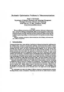
3.1.3 Past and Present Work Several dierent approaches to nding minimum cuts have been investigated; we describe them in the next few sections. Besides putting our work in context, this discussion describes tools that are needed in our minimum cut algorithms. Previously best results, together with our new bounds, are summarized in Figure 3.1, where c denotes the value of the minimum cut. Until recently, the most ecient algorithms were augmenting algorithms that used maximum ow computations. We discuss these algorithms in Section 3.2. As the fastest known algorithms for maximum ow take (mn) time, the best minimum cut algorithms inherited this bound. Gabow showed how augmenting spanning trees rather than ows could nd minimum cuts in O~ (cm) time|an improvement for graphs with small minimum cuts c. Parallel algorithms for the problem have also been investigated, but until now processor bounds have been quite large for unweighted graphs, and no good algorithms for weighted graphs were known. Recently, new and slightly faster approaches to computing minimum cuts without maximum ows appeared. Nagamochi and Ibaraki developed an algorithm for computing sparse


28

minimum cut bounds sequential time processors used in RNC sequential approximation time

unweighted undirected directed 2 previous c2n log nc cm log nm [67] this work c3=2n log n

n4:37

previous this work previous

n2

[115, 73]

this work

weighted undirected directed 2 mn + n2 log n mn log nm [154] [89] 3 n2 log n Unknown

n2

P -complete [79]

(2 + ) in O(m) [148] (1 + ) in O(m)

Figure 3.1: Bounds For the Minimum Cut Problem certi cates (described in Section 3.3) that can be used to speed up the augmenting algorithms. A side eect of their construction is the identi cation of an edge guaranteed not to be in the minimum cut; this leads to a contraction-based algorithm for minimum cuts that is simpler than the augmenting algorithms but has the same O~ (mn) time bound; we discuss this algorithm in Section 3.4. Matula observed that sparse certi cates could also be used to nd a (2 + )-approximation to the minimum cut in linear time; we discuss this algorithm in Section 3.5. After describing these previous results, we contrast our contributions with them in Section 3.6.

3.2 Augmentation Based Algorithms The oldest minimum cut algorithms work by augmenting a dual structure that, when it is maximized, reveals the minimum cut. Note that the undirected minimum cut problem on which we focus is a special case of the directed minimum cut problem. In a directed graph, the value of cut (S; T ) is the number or weight of edges with head in S and tail in T . An algorithm to solve the directed cut problem can solve the undirected one as well: given an

3.2. AUGMENTATION BASED ALGORITHMS

29

undirected graph, replace each edge connecting v and w with two edges, one directed from v to w and the other from w to v. The value of the directed minimum cut in the new graph equals the value of the undirected minimum cut in the original graph.

3.2.1 Flow based approaches The rst algorithm for nding minimum cuts used the duality between s-t minimum cuts and s-t maximum ows [50, 59]. A good discussion of these algorithms can be found in [3]. Since an s-t maximum ow saturates every s-t minimum cut, it is straightforward to nd an s-t minimum cut given an s-t maximum ow|for example, the set of all vertices reachable from the source s in the residual graph of a maximum ow forms one side of such an s-t minimum cut. An s-t maximum ow algorithm can thus be used to nd an s-t minimum ? cut, and minimizing over all n2 possible choices of s and t yields a minimum cut. In 1961, Gomory and Hu [82] introduced the concept of a ow equivalent tree and observed that the minimum cut could be found by solving only n ? 1 maximum ow problems. In their classic book Flows in Networks [60], Ford and Fulkerson comment on the method of Gomory and Hu: Their procedure involved the successive solution of precisely n ? 1 maximal ow problems. Moreover, many of these problems involve smaller networks than the original one. Thus one could hardly ask for anything better. This attitude was prevalent in the following 25 years of work on the minimum cut problem. The focus in minimum cut algorithms was on developing better maximum ow algorithms and better methods of performing series of maximum ow computations. Maximum ow algorithms have become progressively faster over the years. Currently, the fastest algorithms are based on the push-relabel method of Goldberg and Tarjan [78]. Their early implementation of this method runs in O(mn log(n2 =m)) time. Many subsequent algorithms have reduced the running time. Currently, the fastest deterministic algorithms, independently developed by King, Rao and Tarjan [121] and by Phillips and Westbrook [162]) run in O(nm(log n logm n n)) time. Randomization has not helped significantly. The fastest randomized maximum ow algorithm, developed by Cheriyan and Hagerup [28] runs in O(mn + n2 log2 n) time. There appears to be some sort of O(mn) barrier below which maximum ow algorithms cannot go. Finding a minimum cut by directly applying any of these algorithms in the Gomory-Hu approach requires (mn2 ) time.


30

There have also been successful eorts to speed up the series of maximum ow computations that arise in computing a minimum cut. The basic technique is to pass information among the various ow computations so that computing all n maximum ows together takes less time than computing each one separately. Applying this idea, Podderyugin [164], Karzanov and Timofeev [116], and Matula [147] independently discovered several algorithms that determine edge connectivity in unweighted graphs in O(mn) time. Hao and Orlin [89] obtained similar types of results for weighted graphs. They showed that the series of n ? 1 related maximum ow computations needed to nd a minimum cut can all be performed in roughly the same amount of time that it takes to perform one maximum ow computation, provided the maximum ow algorithm used is a non-scaling push-relabel algorithm. They used the fastest such algorithm, that of Goldberg and Tarjan, to nd a minimum cut in O(mn log(n2 =m)) time.

3.2.2 Gabow's Round Robin Algorithm Quite recently, Gabow [67] developed a more direct augmenting-algorithm approach to the minimum cut problem. It is based on a matroid characterization of the minimum cut problem and is analogous to the augmenting paths algorithm for maximum ows. We reconsider the maximum ow problem. The duality theorem of [59] says that the value of the s-t minimum cut is equal to maximum number of edge-disjoint directed s-t paths that can be \packed" in the graph. Gabow's minimum cut algorithm is based on an analogous observation that the minimum cut corresponds to a packing of disjoint directed trees. Gabow's algorithm is designed for directed graphs and is based on earlier work of Edmonds [47]. Given a directed graph and a particular vertex s, a minimum s-cut is a cut (S; S) such that s 2 S and the number of directed edges crossing from S to S is minimized. Since the minimum cut in a graph is a minimum s-cut either in G or in G with all edges reversed, nding a global minimum cut in reduces to nding a minimum s-cut. We de ne a spanning tree in the standard fashion, ignoring edge directions. We de ne a complete k-intersection at s as a set of k edge-disjoint spanning trees that induce an indegree of exactly k on every vertex but s. Gabow's algorithm is based upon the following characterization of minimum cuts: The minimum s-cut of a graph is equal to the maximum number c such that a complete c-intersection at s exists.

3.2. AUGMENTATION BASED ALGORITHMS

31

This characterization corresponds closely to that for maximum ows. Gabow notes that the edges of a complete k-intersection can be redistributed into k spanning trees rooted at and directed away from s. Thus, just as the minimum s-t cut is equal to the maximum number of disjoint paths directed from s to t, the minimum s-cut is equal to the maximum number of disjoint spanning trees directed away from s. Gabow's minimum cut algorithm uses a subroutine called the Round Robin Algorithm (Round-Robin). This subroutine takes as input a graph G with a complete k-intersection. In O(m log(n2=m)) time, it either returns a complete (k + 1)-intersection or proves that the minimum cut is k by returning a cut of value k. Round-Robin can therefore be seen as a cousin of the standard augmenting path algorithm for maximum ows: instead of augmenting by a path, it augments by a spanning tree. We can think of this as attempting to send ow simultaneously from s to every vertex in order to nd the vertex with the smallest possible max- ow from s. Gabow's algorithm for nding a minimum cut is to repeatedly call Round-Robin until it fails. The number of calls needed is just the value c of the minimum cut; thus the total running time of his algorithm is O(cm log(n2 =m)). Gabow's algorithm can be applied to undirected graphs if we replace each undirected edge fu; v g with two directed edges (u; v ) and (v; u). Gabow's algorithm is fastest on graphs with small minimum cuts, and is thus a good candidate for a random sampling approach. We apply this idea in Section 6.3 to develop p linear time approximation algorithms and an O~ (m c)-time exact algorithm for undirected graphs.

3.2.3 Parallel algorithms Parallel algorithms for the minimum cut problem have also been explored, though with much less satisfactory results. For undirected and unweighted graphs, Khuller and Schieber [118] gave an algorithm that uses cn2 processors to nd a minimum cut of value c in O~ (c) time; this algorithm is therefore in NC when c is polylogarithmic in n. For directed unweighted graphs, the RNC matching algorithms of Karp, Upfal, and Wigderson [115] or Mulmuley, Vazirani, and Vazirani [152] can be combined with a reduction of s-t maximum ow problems to matching [115] to yield RNC algorithms for s-t minimum cuts. We can nd a minimum cut by performing 2n of these s-t cut computations in parallel ( x a vertex s, and nd minimum s-v and v -s cuts for each other vertex v ). Unfortunately,

32


the processor bounds are quite large|the best bound, using Galil and Pan's [73] adaptation of [115], is n4:37. These unweighted directed graph algorithms can be extended to work for weighted graphs by treating an edge of weight w as a set of w parallel edges. If W is the sum of all the edge weights then the number of processors needed is proportional to W ; hence the problem is not in RNC unless the edge weights are given in unary. If we combine these algorithms with the scaling techniques of Edmonds and Karp [49], as suggested in [115], the processor count is mn4:37 and the running times are proportional to log W . Hence, the algorithms are not in RNC unless W = n polylog n. The lack of an RNC algorithm is not surprising. Goldschlager, Shaw, and Staples [79] showed that the s-t minimum cut problem on weighted directed graphs is P -complete. In section 4.5.4 we note a simple reduction to their result that proves that the weighted directed minimum cut problem is also P -complete. Therefore, a (randomized) parallel algorithm for the directed minimum cut problem would imply that P NC (RNC), which is believed to be unlikely. An interesting open question is whether Gabow's Round Robin algorithm can be parallelized eciently using maximal matching techniques as for maximum ows; doing so would give a more eective algorithm than the ones based on maximum ows that must consider all source-sink pairs simultaneously.

3.3 Sparse Connectivity Certi cates The augmentation-based algorithms we have just discussed typically examine all the edges in a graph in order to perform one augmentation. It is therefore convenient that we can often preprocess the graph to reduce the number of edges we have to examine. The tool we use is sparse certi cates. Certi cates apply to any monotone increasing property of graphs|one that holds for graph G if it holds for some proper subgraph of G. Given such a property, a sparse certi cate for G is a sparse subgraph that has the property, proving that G has it as well. The advantage is that since the certi cate is sparse, the property can be veri ed more quickly. For example, Eppstein et al [51] give sparsecerti cate techniques that improve the running times of dynamic algorithms for numerous graph problems such as connectivity, bipartitioning, and minimum spanning trees. Minimum cut algorithms can eectively use a particular sparse connectivity certi cate.

3.3. SPARSE CONNECTIVITY CERTIFICATES

33

Using this certi cate, it is often possible to discard many edges from a graph before computing minimum cuts. Discarding edges makes many algorithms (such as Gabow's) run faster. Nagamochi and Ibaraki [155] give a linear-time algorithm called scan- rst search for constructing such a certi cate. A side eect of their algorithm is the identi cation of one edge that is not in the minimum cut; this motivates the development of contraction-based algorithms as an alternative to augmentation-based algorithms. Matula [148] noticed that the certi cate could be used as the centerpiece of a linear time sequential algorithm for nding a (2 + )-approximation to the minimum cut in a graph.

3.3.1 De nition De nition 3.3.1 A sparse k-connectivity certi cate for an n-vertex graph G is a subgraph H of G such that 1. H contains at most kn edges, and

2. H contains all edges crossing cuts of value k or less.

This de nition extends to weighted graphs if we equate an edge of weight w with a set of w unweighted edges with the same endpoints|the bound in size becomes a bound on the total weight of remaining edges. It follows from the de nition that if a cut has value v k in G, then it has the same value v in H . On the other hand, any cut of value greater than k in G has value at least k in H . Therefore, if we are looking for cuts of value less than k in G, we might as well look for them in H , since they are the same. The advantage is that H may have many fewer edges than G. Nagamochi and Ibaraki made this approach feasible by presenting an algorithm that constructs a sparse k-connectivity certi cate in O(m) time on unweighted graphs, independent of k. On weighted graphs, the running time of their algorithm increases to O(m + n log n). Consider, for example, Gabow's minimum cut algorithm from the previous section. It runs in O(cm log(m=n))-time on an n-vertex m-edge graph with minimum cut c. If we knew c, we could use the Nagamochi-Ibaraki algorithm to construct a sparse (c + 1)-connectivity certi cate. This certi cate would have the same minimum cuts of value c as the original graph, but only (c + 1)n edges. Thus Gabow's algorithm would run in O((nc)c log((nc)=n)) time on the certi fcate. The overall time for Gabow's algorithm therefore improves to O(m + c2n log(n=c)). If c is not known, we start by guessing c = 1 and then repeatedly doubling our guess; the running time remains O~ (m +(1+22 +42 + : : : + c2)n) = O~ (m + c2n).

34


The only sparse k-connectivity certi cate known at present is a maximal k-jungle, which we now de ne.

De nition 3.3.2 A k-jungle is a set of k disjoint forests in G. De nition 3.3.3 A maximal k-jungle is a k-jungle such that no other edge in G can be added to any one of the jungle's forests without creating a cycle in that forest.

Lemma 3.3.4 ([154]) A maximal k-jungle contains all the edges in any cut of k or fewer edges.

Proof: Consider a maximal k-jungle J , and suppose it contains fewer than k edges of some cut. Some forest in J must have no edge from this cut. Any cut edge not in J could be added to this forest without creating a cycle, so all cut edges must already be in J .

It follows that a maximal k-jungle is a sparse k-connectivity certi cate, because each forest in the jungle contains at most n ? 1 edges.

3.3.2 Construction The simplest algorithm for constructing a maximal k-jungle is a greedy one: nd and delete a spanning forest from G k times. Nagamochi and Ibaraki give an implementation of this greedy construction called Scan-First-Search. It takes a single pass through the edges and labels them according to which iteration of the greedy algorithm would delete them. This labeling allows them to construct the k-jungle in linear time (or O(m + n log n) time on weighted graphs) by identifying the set of edges with labels at most k. Scan-First-Search constructs certi cates with an important additional property. In a graph with minimum cut c, at least one edge will not be in the rst c forests of the jungle. This edge cannot be in the minimum cut, because by de nition all edges in a cut of value c are contained in the rst c forests. This means that the edge given the largest label by Scan-First-Search will not be in the minimum cut. We will see in the next section that this information can be used eectively to nd minimum cuts. We can also consider parallel sparse certi cate algorithms. These play in important role in several other parts of our work. Cheriyan, Kao, and Thurimella [29] give a parallel sparse certi cate algorithm that runs in O(k log n) time using m + kn processors. It is thus in NC when k = O( polylog n). In Section 5.2, we give a better parallel sparse certi cate

3.4. NAGAMOCHI AND IBARAKI'S CONTRACTION ALGORITHM

35

Figure 3.2: Contraction algorithm that runs in O( polylog n) time using kn processors, and is therefore in NC when k is polynomial.

3.4 Nagamochi and Ibaraki's Contraction Algorithm As we just mentioned, Scan-First-Search has a side eect of identifying an edge that is not in the minimum cut. Nagamochi and Ibaraki [154, 155] use this fact in developing a minimum cut algorithm based on the idea of contraction. If an edge is not in the minimum cut, then its endpoints must be on the same side of the minimum cut. Therefore, if we merge the two endpoints into a single vertex, we will get a graph with one less vertex but with the same minimum cut as the original graph. An example of an edge contraction is given in Figure 3.2. To contract two vertices v1 and v2 we replace them by a vertex v , and let the set of edges incident on v be the union of the sets of edges incident on v1 and v2 . We do not merge edges from v1 and v2 that have the same other endpoint; instead, we create multiple instances of those edges. However, we remove self loops formed by edges originally connecting v1 to v2.


36

Formally, we delete all edges (v1; v2), and replace each edge (v1; w) or (v2 ; w) with an edge (v; w). The rest of the graph remains unchanged. We will use G=(v1; v2) to denote graph G with edge (v1; v2) contracted (by contracting an edge , we will mean contracting the two endpoints of the edge). Extending this de nition, for an edge set F we will let G=F denote the graph produced by contracting all edges in F (the order of contractions is irrelevant up to isomorphism). Remark: Note the dierence between the contraction rule used here and that used in the minimum spanning tree algorithm. There, all edges but the minimum weight edge in a group of parallel edges were deleted; here, all edges in a parallel group remain. Contraction is used as the fundamental operation in Nagamochi and Ibaraki's algorithm NI-Contract shown in Figure 3.3.

Procedure NI-Contract(G) repeat until G has 2 vertices nd an edge (v; w) not in the minimum cut using Scan-first-search let G G=(v; w) return G Figure 3.3: A Generic Contraction-Based Algorithm When NI-Contract terminates, each original vertex has been contracted into one of the two remaining \metavertices." These metavertices de nes a cut of the original graph: each side corresponds to the vertices contained in one of the metavertices. More formally, at any point in the algorithm, we can de ne s(a) to be the set of original vertices contracted to a current metavertex a. Initially s(v ) = v for each v 2 V , and whenever we contract (v; w) to create vertex x we set s(x) = s(v ) [ s(w). We say a cut (A; B ) in the contracted graph corresponds to a cut (A0; B 0 ) in G, where A0 = [a2A s(a) and B 0 = [b2B s(b). Note that a cut and its corresponding cut will have the same value. When the Contraction Algorithm terminates, yielding a graph with two metavertices a and b, we have a corresponding cut (A; B ) in the original graph, where A = s(a) and B = s(b).

Lemma 3.4.1 A cut (A; B) is output by NI-Contract if and only if no edge crossing (A; B) is contracted by the algorithm.

3.5. MATULA'S (2 + )-APPROXIMATION ALGORITHM

37

Proof: The only if direction is obvious. For the other direction, consider two vertices on opposite sides of the cut (A; B ). If they end up in the same metavertex, then there must be a path between them consisting of edges that were contracted. However, any path between them crosses (A; B ), so an edge crossing cut (A; B ) would have had to be contracted. This contradicts our hypothesis.

Corollary 3.4.2 NI-Contract outputs a minimum cut. Proof: By assumption, no edge in the minimum cut is ever contracted. Now note that NI-Contract performs exactly n ? 2 iterations, since the number of vertices is reduced by one each time. Therefore, the running time of NI-Contract is n ? 2

times the time needed to nd a non-minimum-cut edge. Nagamochi and Ibaraki's sparsecerti cate algorithm identi es a non-minimum-cut edge in linear time and therefore yields an implementation of NI-Contract that runs in O(mn) time on unweighted graphs (and O(mn + n2 log n) time on weighted graphs). This implementation improves on maximum

ow based algorithms in terms of both running-time bound and practicality.

3.5 Matula's (2 + )-Approximation Algorithm Matula's (2 + )-approximation algorithm [148] also uses sparse certi cates as its main ingredient. It modi es the approach of Nagamochi and Ibaraki's contraction-based algorithm, using the fact that if many non-minimum-cut edges are found and contracted simultaneously, only a few iterations will be needed. See Procedure Approx-min-cut in Figure 3.4. We describe the algorithm as one that approximates the cut value; it is easily modi ed to nd a cut with the returned value. The basic idea is to nd a sparse certi cate that contains all minimum cut edges and then contract all edges not in the certi cate. The algorithm works quickly because so long as we do not have a good approximation to the minimum cut at hand, we can guarantee that many edges are contracted each time.

Lemma 3.5.1 Given a graph with minimum cut c, the approximation algorithm returns a value between c and (2 + )c.

Proof: Clearly the value is at least c because it corresponds to some cut the algorithm

encounters. For the upper bound, we use induction on the size of G. We consider two cases.


38

Procedure Approx-Min-Cut(G) 1. Let be the minimum degree of G. 2. Let k = =(2 + ). 3. Find a sparse k-connectivity certi cate for G. 4. Construct G0 from G by contracting all non-certi cate edges. 5. Return min(; Approx-Min-Cut(G0)). Figure 3.4: Matula's Approximation Algorithm If < (2 + )c, then since we return a value of at most , the algorithm is correct. On the other hand, if (2 + )c, then k c. It follows that the sparse certi cate we construct contains all the minimum cut edges. Thus no edge in the minimum cut is contracted while forming G0 , so G0 has minimum cut c. By the inductive hypothesis, the recursive call returns a value between c and (2 + )c.

Lemma 3.5.2 In an unweighted graph, the number of levels of recursion in the approxi-

mation algorithm is O(log m).

Proof: If G has minimum degree , it must have at least n=2 edges. On the other hand, the graph G0 that we construct contains at most k(n ? 1) = (n ? 1)=(2+ ) edges. It follows

that each recursive step reduces the number of edges in the graph by a constant factor; thus at a recursion depth of O(log m) the problem can be solved trivially.

Remark: The extra factor above 2 is needed to ensure a signi cant reduction in the number of edges at each stage and thus keep the recursion depth small. The depth of recursion is in fact (?1 log m) and the total work done O(m=).

Corollary 3.5.3 For unweighted graphs, a (2 + )-approximation to the minimum cut can be found in O(m=) time.

Proof: All the steps of Matula's approximation algorithm take O(m) time, except for

nding a sparse certi cate which takes O(m) time using Scan-First-Search.

3.6. NEW RESULTS

39

Remark: Matula's Algorithm can be modi ed to run on weighted graphs if we use the O(m + n log n)-time weighted-graph version of

Scan-First-Search.

We need to use a linear-time preprocessing step (described in Section ??) to ensure that the number of iterations of scanning is O(log n). The resulting algorithm runs in O(m(log n)=) time. We can also consider using the parallel sparse certi cate algorithm of [29]. This algorithm uses m processors and nds a sparse k-connectivity certi cate in O~ (k) time.

Corollary 3.5.4 In a graph with minimum cut c, a (2 + )-approximation to the minimum

cut can be found in O~ (c=) time.

3.6 New Results In the next few chapters, we will present new algorithms for solving the minimum cut problem. Here, we outline the various results we present and compare them to previous best bounds. Consider a graph with m edges, n vertices, and minimum cut c. Many of our results can be seen as circling around the following (quite possibly achievable) goal: develop deterministic linear-time sequential and linear-processor parallel algorithms for nding minimum cuts. In Chapter 4, we develop a powerful new application of the contraction ideas of Section 3.4. Our randomized Recursive Contraction Algorithm is strongly polynomial (see Section 1.3) and runs in O(n2 log3 n) time|a signi cant improvement on the previous O~ (mn) bounds. It is also parallelizable to run in RNC using n2 processors. This gives the rst proof that the minimum cut can be found in RNC . The algorithm can be used to enumerate all approximately minimum cuts in a graph (those with a value any constant factor times the minimum cut's) in polynomial time and in RNC , and to prove that there are few such cuts. These results have important applications in the study of network reliability [170, 36]. For example, we use small-cut enumeration to give the rst fully polynomial time approximation scheme for the all-terminal network reliability problem|the problem of determining the likelihood that a graph becomes disconnected if each of its edges fails with a certain probability. In Chapter 5, we apply derandomization techniques and our cut enumeration theorems to develop a deterministic parallel algorithm for minimum cuts, yielding the rst proof that the minimum cut problem can be solved in NC . To do so, we present a new deterministic parallel algorithm for nding sparse connectivity certi cates. This lets us parallelize

40


Matula's sequential algorithm for nding a (2 + )-approximation to the minimum cut in unweighted graphs. We then show that the minimum cut problem can be reduced in NC to the unweighted minimum cut approximation problem just solved. Sparse certi cates also play an important role in many of the algorithms that follow. In Chapter 6, we use our results on enumeration of small cuts to prove a cut sampling theorem that shows that cuts take predictable values under random sampling. We show how this fact leads to a linear time algorithm for estimating the minimum cut to within (1 + ), thus improving on Matula's approximation algorithm. We also use it to extend our linear processor 2-approximation algorithm to weighted graphs, and to give fast algorithms for maintaining the minimum cut dynamically. In contrast to the Contraction Algorithm which is Monte Carlo, these algorithms can be made Las Vegas. Using a randomized divide-and-conquer scheme for unweighted graphs, we accelerate Gabow's algorithm to run p in O~ (m c) time. In Chapter 10, we extend this approach, developing randomized divide and conquer algorithms for s-t minimum cut and maximum ow problems. We also give applications to other cut-related problems such as minimum s-t cuts and maximum ows. In Chapter 9, we discuss extensions to our Contraction Algorithm. The Recursive Contraction Algorithm can be used to compute (and enumerate) all minimum multiway cuts. The Contraction Algorithm provides a signi cantly faster solution than was previously known, and also gives the rst RNC algorithm for the problem. A variant of the algorithm can be used to construct the cactus representation of minimum cuts in a graph. In two complexity theoretic results, we show that the minimum cut can be found in polynomial time using only O(n) space, and in O(log n) time on an EREW PRAM, matching the lower bound.

Chapter 4

Randomized Contraction Algorithms 4.1 Introduction 4.1.1 Overview of Results In this chapter, we present the Recursive Contraction Algorithm.1 It is a random-selection based algorithm, relying in the fact that a \typical" graph edge is not in the minimum cut. It is therefore analogous to quicksort. While quicksort could use a linear time median nding algorithm to pick a pivot with guaranteed good performance, it instead assumes that a randomly chosen pivot would work well. Similarly, rather than using Nagamochi and Ibaraki's slow algorithm for identifying an edge not in the minimum cut, we pick one at random and assume it is not in the minimum cut. This approach leads to a strongly polynomial algorithm that runs in O(n2 log3 n) time|a signi cant improvement on the previous O~ (mn) bounds. With high probability, our algorithm nds the minimum cut|in fact, it nds all minimum cuts. This suggests that the minimum cut problem may be fundamentally easier to solve than the maximum ow problem. The parallel version of our algorithm runs in polylogarithmic time using n2 processors on a PRAM. It thus provides the rst proof that the minimum cut problem with arbitrary edge weights can be solved in RNC . It is also an ecient RNC algorithm for the minimum cut problem in that the total work it performs is 1

Parts of this chapter appeared in [102] and (joint with Cliord Stein) [110].

41

42

CHAPTER 4. RANDOMIZED CONTRACTION ALGORITHMS

within a polylogarithmic factor of that performed by the best sequential algorithm (namely, the one presented here). In a contrasting result, we show that the directed minimum cut problem is P -complete and thus appears unlikely to have an RNC solution. Our algorithm is extremely simple and, unlike the best ow-based approaches, does not rely on any complicated data structures such as dynamic trees [177]. The most time consuming steps of the sequential version are simple computations on arrays, while the most time consuming steps in the parallel version are sorting and computing connected components. All of these computations can be performed practically and eciently. We have implemented the algorithm and determined that it works well in practice. A drawback of our algorithm is that it is Monte Carlo. Monte Carlo Algorithms give the right answer with high probability but not with certainty. For many problems, such a

aw can be recti ed because it is possible to verify a \certi cate" of the correctness of the output and rerun the algorithm if the output is wrong. This modi cation turns Monte Carlo Algorithms into Las Vegas algorithms that are guaranteed to produce the right answer but have a small probability of taking a long time to do so. Unfortunately, all presently known minimum cut certi cates (such as maximum ows, or the complete intersections of Gabow's algorithm) take just as long to construct when the minimum cut is known as when it is unknown. Thus we can provide no speedup if a guarantee of the minimum cut value is desired. Matching the importance of the Contraction Algorithm is a corollary that follows from its abstract implementation. This corollary bounds the number of approximately minimum cuts in a graph, and is the linchpin of all the sampling theorems and algorithms that follow in Chapters 5, 6, 10, and 10. It also has important implications in analyzing network reliability.

4.1.2 Overview of Presentation We start with an abstract formulation of the Contraction Algorithm in Section 4.2. This extremely simple algorithm has an (1=n2) probability of outputting a minimum cut. It is based on the observation that the edges of a graph's minimum cut form a very small fraction of the graph's edges, so that a randomly selected edge is unlikely to be in the minimum cut. Therefore, if we choose an edge at random and contract its endpoints into a single vertex, the probability is high that the minimum cut will be unaected. We therefore nd the minimum cut by repeatedly choosing and contracting random edges until the minimum

4.1. INTRODUCTION

43

cut is apparent. Moving from the abstract formulation to a more concrete algorithm divides naturally into two stages. In the rst stage, we show how to eciently implement the repeated selection and contraction of edges that forms a single trial of the Contraction Algorithm. Section 4.3 uses a simple adjacency matrix scheme to implement the algorithm in O(n2) time. The second stage deals with the need for multiple trials of the Contraction Algorithm. Given the (1=n2) success probability of the Contraction Algorithm, repeating it O(n2 log n) times gives a high probability of nding the minimum cut in some trial. However, this approach yields undesirably high sequential time and parallel processor bounds of O~ (n4 ). Thus in Section 4.4 we show how the O(n2 log n) necessary trials can share their work so that the total work performed by any one trial is O~ (1). This amortization gives our O~ (n2) sequential time bounds. We next give parallel implementations of the Contraction Algorithm. To achieve parallelism, we \batch together" numerous selections and contractions, so that only a few contraction phases are necessary. We present a simple but slightly inecient (by logarithmic factors) parallel implementation in Section 4.5. This implementation suces to show that minimum cuts of undirected graphs can be found in RNC . In contrast, in Section 4.5.4 we show that the corresponding directed graph problem is P -complete. In section 4.6, we give an asymptotically better (and more practical) implementation of the Contraction Algorithm that runs in linear time sequentially and is more ecient in parallel than our previous implementation. This gives us improved sequential time bounds on certain classes of graphs as well as a more ecient parallel algorithm. In Section 4.7, we return to the abstract description of the Contraction Algorithm and use it to bound the number of approximately minimum cuts in a graph. We then show how the algorithm can be modi ed to nd all the approximately minimum cuts. As an application, in Section 10.1, we give the rst fully polynomial time approximation scheme for the all-terminal network reliability problem of determining the probability that a network remains connected if its edges suer random failures.

44


4.2 The Contraction Algorithm In this section we present an abstract version of the Contraction Algorithm. This version of the algorithm is particularly intuitive and easy to analyze. In later sections, we will describe how to implement it eciently.

4.2.1 Unweighted Graphs For now, we restrict our attention to unweighted multigraphs (i.e., graphs that may have multiple edges between one pair of vertices). The Contraction Algorithm is a variant of Nagamochi and Ibaraki's contraction-based algorithm (presented in Section 3.4). Assume initially that we are given a multigraph G(V; E ) with n vertices and m edges. The Contraction Algorithm is based on the idea that since the minimum cut is small, a randomly chosen edge is unlikely to be in the minimum cut. The Contraction Algorithm, which is described in Figure 4.1, repeatedly chooses an edge at random and contracts it.

Procedure Contract(G) repeat until G has 2 vertices choose an edge (v; w) uniformly at random from G let G G=(v; w) return G Figure 4.1: The Contraction Algorithm

Theorem 4.2.1 A particular minimum cut in G is returned by the Contraction Algorithm ? with probability at least n ?1 = (n?2 ). 2

Proof: Fix attention on some speci c minimum cut (A; B) with c crossing edges. We will

use the term minimum cut edge to refer only to edges crossing (A; B ). From Lemma 3.4.1, we know that if we never select a minimum cut edge during the Contraction Algorithm, then the two vertices we end up with must de ne the minimum cut. Observe that after each contraction, the minimum cut value in the new graph must still be at least c. This is because every cut in the contracted graph corresponds to a cut of the

4.2. THE CONTRACTION ALGORITHM

45

same value in the original graph, and thus has value at least c. Furthermore, if we contract an edge (v; w) that does not cross (A; B ), then the cut (A; B ) corresponds to a cut of value c in G=(v; w); this corresponding cut is a minimum cut (of value c) in the contracted graph. Each time we contract an edge, we reduce the number of vertices in the graph by one. Consider the stage in which the graph has r vertices. Since the contracted graph has a minimum cut of at least c, it must have minimum degree c, and thus at least rc=2 edges. However, only c of these edges are in the minimum cut. Thus, a randomly chosen edge is in the minimum cut with probability at most 2=r. The probability that we never contract a minimum cut edge through all n ? 2 contractions is thus at least

2 n ? 2 n ? 3 2 1 2 2 1? n 1? n ?1 1? 3 = n n? 1 4 3 =

n

!?1

2 = (n?2):

Remark: This bound is tight. In a cycle on n vertices, there are ?n2 minimum cuts, one for

each pair of edges in the graph. Each of these minimum cuts is produced by the Contraction ? Algorithm with equal probability, namely n2 ?1. Remark: An alternative interpretation of the Contraction Algorithm is that we are randomly ranking the edges and then constructing a minimum spanning tree of the graph based on these ranks (using Kruskal's minimum spanning tree algorithm [133]). If we remove the heaviest edge in the minimum spanning tree, the two components that result have an (n?2) chance of de ning a particular minimum cut. This intuition forms the basis of the implementation of Section 4.6, as well as for certain dynamic approximation algorithms in Section 10.5. The Contraction Algorithm can be halted when k vertices remain. We refer to this as contraction to k vertices. The following result is an easy extension of Theorem 4.2.1:

Corollary 4.2.2 A particular minimum cut (A; B) survives contraction to k vertices with ?? probability at least k = n = ((k=n)2). 2

2


46

4.2.2 Weighted Graphs Extending the Contraction Algorithm to weighted graphs is simple. For a given weighted graph G, we consider a corresponding unweighted multigraph G0 on the same set of vertices. An edge of weight w in G is mapped to a collection of w parallel unweighted edges in G0. The minimum cuts in G and G0 are the same, so it suces to run the Contraction Algorithm on G0. We choose a pair of vertices to contract in G0 by selecting an edge of G0 uniformly at random. Therefore, the probability that we contract u and v is proportional to the number of edges connecting u and v in G0, which is just the weight of the edge (u; v ) in G. This interpretation leads to the weighted version of the Contraction Algorithm given in Figure 4.2.

Procedure Contract(G) repeat until G has 2 vertices choose an edge (v; w) with probability proportional to the weight of (v; w) let G G=(v; w) return G Figure 4.2: The Weighted Contraction Algorithm The analysis of this algorithm follows immediately from the unweighted case.

Corollary 4.2.3 The Weighted Contraction Algorithm outputs a particular minimum cut of G with probability (1=n2).

4.3 Implementing the Contraction Algorithm We now turn to implementing the algorithm described abstractly in the previous section. First, we give a version that runs in O(n2) time and space. Later, we shall present a version that runs in O(m) time and space with high probability and is also parallelizable. This rst method, though, is easier to analyze, and its running time does not turn out to be the dominant factor in our analysis of the time to nd minimum cuts. To implement the Contraction Algorithm we use an n n weighted adjacency matrix W . The entry W (u; v) contains the weight of edge (u; v), which can equivalently be viewed

4.3. IMPLEMENTING THE CONTRACTION ALGORITHM

47

as the number of multigraph edges connecting u and v . If there is no edge connecting u and v then W (u; v ) = 0. We also maintain the total (weighted) degree D(u) of each vertex u, thus D(u) = Pv W (u; v). We now show how to implement two steps: randomly selecting an edge and performing a contraction.

4.3.1 Choosing an Edge A fundamental operation that we need to implement is the selection of an edge with probability proportional to its weight. A natural method is the following. First, from edges e1; : : :; em with weights w1 ; : : :; wm; construct cumulative weights Wk = Pki=1 wi. Then choose an integer r uniformly at random from 0; : : :; Wm and use binary search to identify the edge ei such that Wi?1 r < Wi . This can easily be done in O(log W ) time. While this bound is not a strongly polynomial bound since it depends on the edge weights being small, we will temporarily ignore this issue. For the time being, we assume that we have a black-box subroutine called Random-Select. The input to Random-Select is a cumulative weight array of length m. Random-Select runs in O(log m) time and returns an integer between 1 and m, with the probability that i is returned being proportional to wi. In practice the lack of strong polynomiality is irrelevant since implementors typically pretend that their system-provided random number generator can be made to return numbers in an arbitrarily large range by scaling. We provide theoretical justi cation for using Random-Select by giving a strongly polynomial implementation of it in the appendix (Section A.3). We now use Random-Select to nd an edge to contract. Our goal is to choose an edge (u; v ) with probability proportional to W (u; v ). To do so, choose a rst endpoint u with probability proportional to D(u), and then once u is xed choose a second endpoint v with probability proportional to W (u; v). Each of these two choices requires O(n) time to construct a cumulative weight array and one O(log n)-time call to Random-Select, for a total time bound of O(n). The following lemma, similar to one used by Klein, Plotkin, Stein and Tardos [122], proves the correctness of this procedure.

Lemma 4.3.1 If an edge is chosen as described above, then Pr[(u; v) is chosen] is proportional to W (u; v ):


48

Proof: Let = Pv D(v). Then Pr[choose(u; v )] = Pr[choose u] Pr[choose (u; v ) j chose u] + Pr[choose v ] Pr[choose (u; v ) j chose v ] D ( u) W (u; v) + D(v) W (u; v) = D(u) D(v) = 2W (u; v )

/ W (u; v):

4.3.2 Contracting an Edge Having shown how to choose an edge, we now show how to implement a contraction. Given W and D, which represent a graph G, we explain how to update W and D to re ect the contraction of a particular edge (u; v ). Call the new graph G0 and compute its representation via the algorithm of Figure 4.3.2. Intuitively, this algorithm moves all edges incident on v to u. The algorithm replaces row u with the sum of row u and row v , and replaces column u Procedure to contract edge (u; v )

Let D(u) D(u) + D(v) ? 2W (u; v) Let D(v) 0 Let W (u; v) W (v; u) 0 For each vertex w except u and v Let W (u; w) W (u; w) + W (v; w) Let W (w; u) W (w; u) + W (w; v) Let W (v; w) W (w; v) 0 Figure 4.3: Contracting an Edge with the sum of column u and column v . It then clears row v and column v . W and D now represent G0 , since any edge that was incident to u or v is now incident to u and any two

4.4. THE RECURSIVE CONTRACTION ALGORITHM

49

edges of the form (u; w) and (v; w) for some w have had their weights added. Furthermore, the only vertices whose total weighted degrees have changed are u and v , and D(u) and D(v) are updated accordingly. Clearly, this procedure can be implemented in O(n) time. Summarizing this and the previous section, we have shown that in O(n) time we can choose an edge and contract it. This yields the following result:

Corollary 4.3.2 The Contraction Algorithm can be implemented to run in O(n2) time. Observe that if the Contraction Algorithm has run to completion, leaving just two vertices u and v , then we can determine the weight of the implied cut by inspecting W (u; v ). We can in fact implement the Contraction Algorithm using only O(m) space. We do so by maintaining an adjacency list representation. All the edges incident to vertex v are in a linked list. In addition, we have pointers between the two copies of the same edge (v; w) (in the adjacency list of vertex v ) and (w; v ) (in the adjacency list for w). When v and w are merged, we traverse the adjacency list of v, and for each edge (v; u) nd the corresponding edge (u; v ) and rename it to (u; w). Note that as a result of this renaming the adjacency lists will not be sorted. To handle this problem, whenever we choose to merge two vertices, we can merge their adjacency lists by using a bucket sort into n buckets based on the edges' other endpoints; the time for this merge thus remains O(n) and the total time for the algorithm remains O(n2 ). In the worst case m = (n2 ), but for sparse graphs using this approach will save space.

4.4 The Recursive Contraction Algorithm The Contraction Algorithm can be used by itself as an algorithm for nding minimum cuts. Since each trial has an (n?2) probability of success, performing O(n2 log n) trials will give a high probability of nding a minimum cut. However, the resulting sequential running time of (n4 log n) is excessive. We therefore wrap the Contraction Algorithm within the Recursive Contraction Algorithm. The idea of this new algorithm is to share the bulk of the work among the O(n2 log n) Contraction Algorithm trials so as to reduce the total work done. We begin with some intuition as to how to speed up the Contraction Algorithm. Consider the contractions performed in one trial of the Contraction Algorithm. The rst contraction has a reasonably low probability of contracting an edge in the minimum cut, namely

50


2=n. On the other hand, the last contraction has a much higher probability of contracting an edge in the minimum cut, namely 2=3. This observation suggests that the Contraction Algorithm works well initially, but has poorer performance later on. We might improve our chances of success if, after partially contracting the graph, we switched to a (possibly slower) algorithm with a better chance of success on what remains. One possibility is to use one of the deterministic minimum cut algorithms, such as NI-Contract, and this approach indeed yields some improvement. However, a better observation is that an algorithm that is more likely to succeed than the Contraction Algorithm is two trials of the Contraction Algorithm. Therefore, we now use the Contraction Algorithm as a subroutine Contract(G; k), that accepts a weighted graph G and a parameter k and, in O(n2 ) time, returns a contraction of ?? G to k vertices. With probability at least k2 = n2 (Corollary 4.2.2), a particular minimum cut of the original graph will be preserved in the contracted graph. In other words, no vertices on opposite sides of this minimum cut will have been merged, so there will be a minimum cut in the contracted graph corresponding to the particular minimum cut of the original graph. Consider the Recursive Contraction Algorithm described in Figure 4.4. We perform two independent trials. In each, we rst partially contract the graph, but not so much that the likelihood of the cut surviving is too small. By contracting the graph until it p has n= 2 vertices, we ensure a roughly 50% probability of not contracting a minimum cut edge, so we expect that on the average one of the two attempts will avoid contracting a minimum cut edge. We then recursively apply the algorithm to each of the two partially contracted graphs. As described, the algorithms returns only a cut value; it can easily be modi ed to return a cut of the given value. Alternatively, we might want to output every cut encountered, hoping to enumerate all the minimum cuts. We now analyze the running time of this algorithm.

Lemma 4.4.1 Algorithm Recursive-Contract runs in O(n2 log n) time and uses O(n2) or O(m log(n2 =m)) space (depending on the implementation Contract).

Proof: One level of recursion consists of two independent trials of contraction of G to p p

n= 2 vertices followed by a recursive call. Performing a contraction to n= 2 vertices can be implemented by Algorithm Contract from Section 4.3 in O(n2) time. We thus have the


51

Procedure Recursive-Contract(G; n) input A graph G of size n. if G has 2 vertices a and b then return the weight of the corresponding cut in G else repeat twice

p G; n= 2) p Recursive-Contract(G0; n= 2).

G0

Contract(

return the smaller of the two resulting values. Figure 4.4: The Recursive Contraction Algorithm following recurrence for the running time:

T (n) = 2

n2 + T

n p : 2

(4.1)

This recurrence is solved by

T (n) = O(n2 log n); and the depth of the recursion is 2 log2 n.

Note that we have to store one graph at each level of the recursion, where the graph at the p level has nk = n= 2k vertices. If we use the original adjacency matrix implementation P of the Contraction Algorithm, then the space required is O( k n2 =2k ) = O(n2 ). To improve the space bound, we can use the linear-space variant of procedure Contract. Since at each level the graph has no more than min(m; n2k) edges and can be stored using O(min(m; n2k )) P space, the total storage needed is k O(min(m; n2k )) = O(m log(n2=m)).

kth

Remark: This analysis shows why the running time of the Contraction Algorithm is not

the bottleneck in the Recursive Contraction Algorithm. We shall later present a linear time (in the number of edges) implementation of the Contraction Algorithm. However, since the recurrence we formulate must apply to the contracted graphs as well, there is no a priori bound on the number of edges in the graphs we encounter as subproblems. Therefore r2 is the only bound we can put on the number of edges, and thus on the time needed to perform p a contraction to r= 2 vertices, in the the r-vertex graphs we encounter in the recursion.

52


Furthermore, the existence of n2 leaves in the recursion tree gives a lower bound of n2 on the running time of Recursive-Contract, regardless of the speed of Contract. This is why the linear-time implementation of Contract that we shall give in Section 4.5 provides no speedup in general. We now analyze the probability that the algorithm nds the particular minimum cut we are looking for. We will say that the Recursive Contraction Algorithm nds a certain minimum cut if that minimum cut corresponds to one of the leaves in the computation tree of the Recursive Contraction Algorithm. Note that if the algorithm nds any minimum cut then it will certainly output some minimum cut.

Lemma 4.4.2 The Recursive Contraction Algorithm nds a particular minimum cut with probability (1= log n).

Proof: Suppose that a particular minimum cut has survived up to some particular node in

the recursion tree. It will survive to a leaf below that node if two criteria are met: it must survive one of the graph contractions at this node, and it must be found by the recursive call following that contraction. Each of the two branches thus has a success probability equal to the product of the probability that the cut survives the contraction and the probability that the recursive call nds the cut. The probability that the cut survives the contraction is, by Corollary 4.2.2, at least

p

p

(n= 2)(n= 2 ? 1) = 1 ? O(1=n): n(n ? 1) 2 This yields a recurrence P (n) for a lower bound on the probability of success on a graph of size n: 2 ? O(1=n): (4.2) P (n) = 1 ? 1 ? 21 P pn 2 Assume for now that the O(1=n) is factor is negligible. We solve this recurrence through p a change of variables. Letting pk = P ( 2k ), the recurrence above can be rewritten and simpli ed as pk+1 = pk ? 41 p2k :

Let zk = 4=pk ? 1, so pk = 4=(zk + 1). Substituting this in the above recurrence and solving for zk+1 yields zk+1 = zk + 1 + 1=zk :


53

It follows by induction that

k < zk < k + Hk?1 + 3; where Hk is the kth harmonic number [126]. Thus zk = k + O(log k) and pk = 4=(zk + 1) = 4=(k + O(log k) + 1) = (1=k). It follows that P (n) = p2 log2 n = (1= log n): In other words, one trial of the Recursive Contraction Algorithm nds any particular minimum cut with probability (1= log n). To handle the O(1=n) term that we ignored, we can make a small change to procedure p p Recursive-Contract and contract from n vertices to 1 + n= 2 instead of n= 2 before recursing. This makes the probability that a minimum cut survives exceed 1=2, but also keeps a depth of recursion of O(log n), so the analysis of P (n) becomes completely correct without changing the running time analysis.

Remark: Those familiar with branching processes might see that we are evaluating the

probability that the extinction of contracted graphs containing the minimum cut does not occur before depth 2 log n.

Theorem 4.4.3 All minimum cuts in an arbitrarily weighted undirected graph with n ver-

tices and m edges can be found in O(n2 log3 n) time and O(m log(n2 =m)) space (Monte Carlo).

Proof: It is known ([44] and [140], see also Theorem 4.7.6) that there are at most ?n2 min-

imum cuts in a graph. Repeating Recursive-Contract O(log2 n) times gives an O(1=n4) chance of missing any particular minimum cut. Thus our chance of missing any one of the ? at most n2 minimum cuts is negligible.

It is noteworthy that unlike the best algorithms for maximum ow, Recursive-Contract uses no non-trivial data structures. The algorithm has proven to be practical and easy to code. We can view the running of the Recursive Contraction Algorithm as a binary computation tree, where each vertex represents a graph with some of its edges contracted and each p edge represents a contraction by a factor of 2. A leaf in the tree is a contracted graph with 2 metavertices and de nes a cut, potentially a minimum cut. The depth of this tree is 2 log2 n, and it thus has n2 leaves. This shows that the improvement over the direct use

54


of n2 trials of the Contraction Algorithm comes not from generating a narrower tree (those trials also de ne a \tree" of depth 1 with n2 leaves), but from being able to amortize the cost of the contractions used to produce a particular leaf. If it suces to output only one minimum cut, then we can keep track of the smallest cut encountered as the algorithm is run and output it afterwards in O(n) time by unraveling the sequence of contractions that led to it. If we want to output all the minimum cuts, then the output might in fact become the dominant factor in the running time: there could be n2 such cuts, each requiring O(n) time to output as a list of vertices on each side of the cut. This problem is made even worse by the fact that some minimum cuts may be produced many times by the algorithm. Applegate [10] observed that there is a simple hashing technique that can be used to avoid outputting a cut more than once. At the beginning, assign to each vertex a random O(log n)-bit key. Whenever two vertices are merged by contractions, combine their keys with an exclusive-or. At a computation leaf in which there are only two vertices, the two keys of those vertices form an identi er for the particular cut that has been found. With high probability, no two distinct cuts we nd will have the same identi ers. Thus by checking whether an identi er has already been encountered we can avoid outputting any cut that has already been output. An alternative approach to outputting all minimum cuts is to output a concise representation of them; this issue is taken up in Section 9.3.

4.5 A Parallel Implementation We now show how the Recursive Contraction Algorithm can be implemented in parallel (RNC ). To do so, we give an m processor RNC implementation of the Contract by eliminating the apparently sequential nature of the selection and contraction of edges one at a time. Parallelizing Recursive-Contract is then easy. As a rst step, we will show how a series of selections and contractions needed for the Contraction Algorithm can be implemented in O~ (m) time. The previous O(n2) time bound arose from a need to update the graph after each contraction. We circumvent this problem by grouping series of contractions together and performing them all simultaneously. As before, we focus initially on unweighted multigraphs. We start by giving our algorithms as sequential ones, and then show how they can be parallelized.

4.5. A PARALLEL IMPLEMENTATION

55

4.5.1 Using A Permutation of the Edges We reformulate the Contraction Algorithm as follows. Instead of choosing edges one at a time, we begin by generating a uniform random permutation L of the edges. Imagine contracting edges in the order in which they appear in the permutation, until only two vertices remain. This algorithm is clearly equivalent to the abstract formulation of the Contraction Algorithm. We can immediately deduce that with probability (n?2), a random permutation will yield a contraction to two vertices that determine a particular minimum cut. Given a random permutation L of the edges, contracting the edges in the order speci ed by the permutation until two vertices remain corresponds to identifying a pre x L0 of L such that contracting the edges in L0 yields a graph with exactly two vertices. Equivalently, we are looking for a pre x L0 of edges such that the graph H = (V; L0) has exactly two connected components. Binary search over L can identify this pre x, because any pre x that is too short will yield more than two connected components, and any pre x that is too long will yield only one. The correct pre x can therefore be determined using O(log m) connected component computations, each requiring O(m + n) time. The total running time of this algorithm (given the permutation) is therefore O(m log m). We can improve the running time by reusing information between the dierent connected component computations. Given the initial permutation L, we rst use O(m + n) time to identify the connected components induced by the rst m=2 edges. If exactly two connected components are induced, we are done. If only one connected component is induced, then we can discard the last m=2 edges because the desired pre x ends before the middle edge, and recurse on the rst half of L. If more than two connected components are induced, then we can contract the rst m=2 edges all at once in O(m) time by nding the connected components they induce and relabeling the last m=2 edges according to the connected components, producing a new, m=2 edge graph on which we can continue the search. Either way, in O(m + n) time, we have reduced the number of edges to m=2. Since the graph is assumed to be connected, we know that n m as m decreases. Therefore, if we let T (m) be the time to execute this procedure on a graph with m edges, then T (m) T (m=2) + O(m), which has solution T (m) = O(m). In Figure 4.5 we formally de ne this Compact subroutine. We describe Compact with a parameter k describing the goal number of vertices. Our running time analysis assumes that k is two. Running times clearly do not increase when k is larger. Recall the notation G=F that denotes the result of contracting graph G by edge set F . We extend this de nition to as


56

Procedure Compact(G; L; k) input: A graph G and list of edges L and a parameter k if G has k vertices or L = ; then else

return G

Let L1 and L2 be the rst and second halves of L Find the connected components in graph H = (V; L1) if H has fewer than k components

then else

return Compact(G; L1; k) return Compact(G=L1; L2=L1; k). Figure 4.5: Procedure Compact

follows. If E is a set of edges in G, then E=F denotes a corresponding set of edges in G=F : an edge ([; v )][w] 2 E is transformed in E=F to an edge connecting the vertices containing v and w in G=F . Constructing E=F requires merging edges with identical endpoints. Since each endpoint is an integer between 1 and n, we can use a linear-time sorting algorithm, such as bucket sort, to merge edges, and thus Compact runs in O(m) time.

4.5.2 Generating Permutations using Exponential Variates The only remaining issue is how to generate the permutation of edges that is used as the list L in Compact. To show how the permutation generation can be accomplished in RNC, we give in this section an approach to the problem that is easy to explain but gives somewhat worse than optimum bounds in both theory and practice. In Section 4.6, we describe a more ecient (and practical) but harder to analyze approach. For unweighted graphs, a simple method is to assign each edge a score chosen uniformly at random from the unit interval, and then to sort the edges according to score. To extend this approach to weighted graphs, we use the equivalence between an edge of weight w in a weighted graph and a set of w parallel edges in the natural corresponding unweighted

4.5. A PARALLEL IMPLEMENTATION

57

multigraph. We use the term multiedge to mean an edge of the multigraph corresponding to the weighted graph, and simulate the process of generating a random permutation of the multiedges. The entire multiedge permutation is not necessary in the computation, since as soon as a multiedge is contracted, all the other multiedges with the same endpoints vanish. In fact, all that matters is the earliest place in the permutation that a multiedge with particular endpoints appears. This information suces to tell us in which order vertices of the graph are merged: we merge u and v before x and y precisely when the rst (u; v ) multiedge in the permutation precedes the rst (x; y ) multiedge in the permutation. Thus our goal is to generate an edge permutation whose distribution re ects the order of rst appearance of endpoints in a uniform permutation of the corresponding multigraph edges. As in the unweighted case, we can consider giving each multiedge a score chosen uniformly at random from a large ordered set and then sorting according to score. In this case, the rst appearance in the permutation of a multiedge with w copies is determined by the minimum of w randomly chosen scores. We can therefore generate an appropriately distributed permutation of the weighted edges if we give an edge of weight w the minimum of w randomly chosen scores and sort accordingly. Consider multiplying each edge weight by some value , so that an edge of weight w corresponds to w multiedges. This scales the value of the minimum cut without changing its structure. Suppose we give each multiedge a score chosen uniformly at random from the continuous interval [0; ]. The probability distribution for the minimum score X among w edges is then Pr[X > t] = (1 ? t=)w : If we now let become arbitrarily large, the distribution converges to one in which an edge of weight w receives a score chosen from the exponential distribution Pr[X > t] = e?wt: Thus if we can generate an exponential random variable in O(1) time, then we can generate a permutation in O(m) time. As in the unweighted case, we do not actually have to sort based on the scores: once scores are assigned we can use median nding to split the edge list as needed by Compact in O(m) time. If all we have is coin ips, it is possible to use them to sample from an approximately exponential distribution in logarithmic time and introduce a negligible probability of error in the computation. As we shall be describing a better method later, we refer the reader to the appendix (Section A.4) for details.

58


4.5.3 Parallelizing the Contraction Algorithm Parallelizing the previous algorithm is simple. To generate the permutation, given a list of edges, we simply assign one processor to each edge and have it generate the (approximately) exponentially distributed score for that edge in polylogarithmic time. We then use a parallel sorting algorithm on the resulting scores. Given the permutation, it is easy to run Compact in parallel. RNC algorithms for connected components exist that use m= log n processors and run in O(log n) time on a CRCW PRAM [175] or even on the EREW PRAM [88]. Procedure Compact, which terminates after O(log n) iterations, is thus easily seen to be parallelizable to run in O(log2 n) time using m processors. As a result, we have the following:

Theorem 4.5.1 Contract can be implemented to run in RNC using m processors on an m edge graph.

Using the linear-processor RNC implementation of Contract, we can give the rst RNC algorithm for the minimum cut problem.

Theorem 4.5.2 The minimum cut problem can be solved in RNC using n2 processors and O(n2 log3 n) space.

Proof: Consider the computation tree generated by Recursive-Contract. The sequen-

tial algorithm examines this computation tree using a depth- rst traversal of the tree nodes. To solve the problem in parallel, we instead use a breadth- rst traversal. The subroutine Contract has already been parallelized. We can therefore evaluate our computation tree in a breadth- rst fashion, taking only polylogarithmic time to advance one level. The space required is now the space needed to store the entire tree. The sequential running time recurrence T (n) also provides a recursive upper bound on the space needed to store the tree. Thus the space required is O(n2 log3 n) (on the assumption that we perform all O(log2 n) trials of Recursive-Contract in parallel).

4.5.4 Comparison to Directed Graphs The previous results indicate a distinction between minimum cut problems on directed and undirected graphs. In a directed graph, the s-t minimum cut problem is the problem of nding a partition of the vertices into two sets S and T , with s 2 S and t 2 T , such that the weight of edges going from S to T is minimized. Note that the weights of edges going from

4.6. A BETTER IMPLEMENTATION

59

T to S is not counted in the value of the cut. The s-t minimum cut problem on directed graphs was shown to be P -complete [79]. A similar result holds for the global minimum cut problem:

Lemma 4.5.3 The global minimum cut problem is P -complete for directed graphs. Proof: Given an algorithm the nds global minimum cuts, we nd a minimum s-t cut as

follows. We add, for each vertex v , directed edges of in nite weight from t to v and from v to s. The global minimum cut in this modi ed graph must now have s 2 S and t 2 T , for otherwise some of the edges of in nite weight would cross in the cut. Hence the global minimum cut must be a minimum s-t cut of the original graph.

The minimum cut problem is therefore in the family of problems, such as reachability, that presently have dramatically dierent diculties on directed and undirected graphs [100, 159]. Indeed, in Section 9.6 we show that the minimum cut can be found in O(log n) time, even on an EREW PRAM.

4.6 A Better Implementation 4.6.1 Iterated Sampling We now discuss a harder to analyze (but easier to implement) version of the Contraction Algorithm based on permutations. It has several advantages, both theoretical and practical, over the exponential variates approach. First, it does not need to approximate logarithms. Although we have argued that such a computation can be done in O(log n) time in theory, in practice we would like to avoid any use of complicated oating point operations. Second, the sequential implementation runs in linear time rather than O(m polylog m) time. As we have discussed, this new implementation will not produce any improvement in the worstcase running time of the Recursive Contraction Algorithm on arbitrary graphs, since such graphs might have n2 edges. However, it does give a slightly improved time bounds for nding minimum cuts in certain classes of sparse graphs. Yet another advantage is that it uses O(m) space without using the pointers and linked lists needed in the O(m)-space adjacency list version of the sequential implementation in Section 4.3. Finally, the parallel version of this algorithm performs less work (by several polylogarithmic factors) than the exponential variates implementation.


60

As in the exponential variates algorithm of Section 4.5.2, we generate a permutation by treating each weighted edge as a collection of parallel unweighted edges. Rather than generating scores, we repeatedly simulate the uniform selection of a multigraph edge by choosing from the graph edges with probabilities proportional to the edge weights; the order of selection then determines the order of rst appearance of multigraph edges (this approach is directly analogous to our analysis of the Contraction Algorithm for weighted graphs in Section 4.2.2. Suppose we construct an array of m cumulative edge weights as we did in the sequential algorithm. We can use the procedure Random-Select (Appendix A.3) to select one edge at random in O(log m) amortized time and then contract it. Since it takes O(m) time to recompute the cumulative distribution, it is undesirable to do so each time we wish to sample an edge. An alternative approach is to keep sampling from the original cumulative distribution and to ignore edges if we sample them more than once. Unfortunately, to make it likely that all edges have been sampled once, we may need a number of samples equal to the sum of the edge weights. For example, if one edge contains almost all the weight in the graph, we will continually select this edge. We solve this problem by combining the two approaches and recomputing the cumulative distribution only occasionally. For the time being, we shall assume that the total weight of edges in the graph is polynomial in n.

Procedure Iterated-Sampling(G; k) input A graph G Let s = n1+ , for some constant 0 < < 1. repeat Compute cumulative edge weights in G Let M be a list of s edge selections using Random-Select on the cumulative edge weights G Compact(G; M; k)

until G has k vertices Figure 4.6: Iterated-Sampling Implementation


61

An implementation of the Contraction Algorithm called Iterated-Sampling is presented in Figure 4.6. Take to be any constant (say 1/2). We choose s = n1+ edges from the same cumulative distribution, contract all theses edges at once, recompute the cumulative distribution and repeat. We now analyze the running time of Iterated-Sampling. We must be somewhat careful with this analysis because we call Iterated-Sampling on very small problems that arise in the recursive computation of Recursive-Contract. Therefore, events that are \low probability" may actually happen with some frequency in the context of the original call to Recursive-Contract. We will therefore have to amortize these \low probability" events over the entire recursion. To do so, we use the following lemmas:

Lemma 4.6.1 The worst case running time of Iterated-Sampling is O(n3). Proof: Each iteration requires O(m + s log n) = O(n2) time. The rst edge chosen in each

iteration will identify a pair of vertices to be contracted; thus the number of iterations is at most n.

Lemma 4.6.2 Call an iteration of Iterated-Sampling successful if it nishes contracting

the graph or if it reduces the total weight in the graph by a factor of 2n=s = O(n? ) for the next iteration. Then the probability that an iteration is not successful is e? (n).

Proof: We assume that the weight reduction condition does not hold, and show that the

iteration must then be likely to satisfy the other success condition. Consider contracting the edges as they are chosen. At any time, call an edge good if its endpoints have not yet been merged by contractions. Since Iterated-Sampling is not aware of the contractions, it may choose non-good edges. The total weight of edges in the next iteration is simply the total weight of good edges at the end of this iteration. Suppose that at the start of the iteration the total (all good) weight is W . By assumption, at the end the total good weight exceeds 2nW=s. Since the total good weight can only decrease as contractions occur, we know that the total good weight at any time during this iteration exceeds 2nW=s. It follows that each time an edge is selected, the probability that it will be a good edge exceeds 2n=s. Given that we perform s selections, the expected number of good selections exceeds 2n. Then by the Cherno bound (Appendix A.2), the probability that fewer than n good edges are selected is exponentially small in n.

62


The number of contractions performed in an iteration is simply the number of good edges selected. Thus, by performing more than n good selections, the iteration will necessarily nish contracting the graph.

Corollary 4.6.3 On an n-vertex graph, the expected running time of Iterated-Sampling is O(m + n1+ ).

Proof: Recall our assumption that W = nO(1). Thus, in the language of Lemma 4.6.2,

after a constant number k of successful iterations Iterated-Sampling will terminate. The previous lemma proves that for some constant n, the probability of a successful iteration is p 1=2. Therefore, the number of iterations needed to terminate has a negative binomial distribution B ? (k; p), with expectation k=p 2k, a constant (see Appendix A.1 for details). Since each iteration takes O(m + n1+ ) time, the result follows. The above result suces to prove all the expected running time bound in the following sections; for a high probability time bound we need the following two corollaries:

Corollary 4.6.4 On an n-vertex graph, the number of iterations before completion of Iterated-Sampling is at most t with probability 1 ? e? (nt). Proof: As was just argued, we terminate after a constant number of successful iterations. Thus the only way for it to take more than t iterations is for there to be roughly t failures, each with probability e? (n) according to Lemma 4.6.2.

Corollary 4.6.5 On an n vertex graph, the running time of Iterated-Sampling is O(t(m+ n1+ )) with probability 1 ? e? (nt). Note that we set s = n1+ to make the analysis easiest for our purposes. A more natural setting is s = m= log m since this balances the time spent sampling and the time spent recomputing cumulative edge weights. Setting s = m= log m yields the same time bounds, but the analysis is more complicated.

4.6.2 An O(n2 )-Approximation We now show how to remove the assumption that W is polynomial in n, while maintaining the same running times. The obstacle we must overcome is that the analysis of the number


63

of iterations of Iterated-Sampling deals with the time to reduce W to zero. If W is arbitrarily large, this reduction can take arbitrarily many iterations. To solve the problem, we use a very rough approximation to the minimum cut to ensure that Corollary 4.6.3 applies even when the edge weights are large. Let w be the largest edge weight such that the set of edges of weight greater than or equal to w connects all of G. This is just the minimum weight of an edge in a maximum spanning tree of G, and can thus be identi ed in O(m log n) time using any standard minimum spanning tree algorithm [41]. Even better, it can be identi ed in O(m) time by the Compact subroutine if we use the inverses of the actual edge weights as edge scores to determine the order of edge contraction. It follows that any cut of the graph must cut an edge of weight at least w, so the minimum cut has weight at least w. It also follows from the de nition of w that there is a cut that does not cut any edge of weight exceeding w. This means that the graph has a cut of weight at most mw and hence the minimum cut has weight at most mw n2w. This guarantees that no edge of weight exceeding n2 w can possibly be in the minimum cut. We can therefore contract all such edges, without eliminating any minimum cut in the graph. Afterwards the total weight of edges in the graph is at most n4 w. Since we merge some edges, we may create new edges of weight exceeding n2 w; these could be contracted as well but it is easier to leave them. Consider running Iterated-Sampling on this reduced graph. Lemma 4.6.2 holds unchanged. Since the total weight is no longer polynomial, Corollary 4.6.3 no longer holds as a bound on the time to reduce the graph graph weight to 0. However, it does hold as bounds on the number of iterations needed to reduce the total remaining weight by a factor of n4 , so that it is less than w. Since the minimum cut exceeds w, the compacted graph at this point can have no cuts, since any such cut would involve only uncontracted edges and would thus have weight less than w. In other words, the graph edges that have been sampled up to this point must suce to contract the graph to a single vertex. This proves that Corollary 4.6.4 and 4.6.5 also hold in the case of arbitrary weights.

4.6.3 Sequential Implementation Using the new, O(m + n1+ )-time algorithm allows us to speed up Recursive-Contract on graphs with excluded dense minors.2 Assume that we have a graph such that all r-vertex 2 A minor of G is a graph that can be derived from G by deleting edges and vertices and contracting edges.

64


minors have O(r2?) edges for some some positive constant . Then we can be sure that at all times during the execution of the Recursive Contraction Algorithm the contracted graphs of r vertices will never have more than r2? edges. We use the O(m + n1+ ) time bound of Corollary 4.6.3 to get an improved running time for Recursive-Contract.

Theorem 4.6.6 Let G have the property that all r-vertex minors have O(r2?) edges for some some positive constant . Then with high probability the Recursive Contraction algorithm nds a minimum cut of G in O(n2 log2 n) time.

Proof: We need to bound the time spent in all calls to Iterated-Sampling over all the var-

ious calls made to Contract in the computation tree of Recursive-Contract. An expected time analysis is quite easy. By Corollary 4.6.3, the expected time of Iterated-Sampling on a problem with m edges is O(m + n1+ ). By the assumption about graph minors, this means that the expected running time of Contract on an r-vertex subproblem will be O(r2?). This gives us an improved recurrence for the running time:

p T (n) = 2(n2? + T (n= 2)):

This recurrence solve to T (n) = O(n2). To improve the analysis to a high probability result we must perform a global analysis of the recurrence as we did for the minimum spanning tree algorithm. Consider two cases. At depths less than log n in the computation tree, where the smallest graph has at least pn vertices, Corollary 4.6.5 says that the expected time bound for Iterated-Sampling is in fact a high probability time bound, so the recurrence holds with high probability at each node high in the computation tree. Below depth log n, some of the problems are extremely small. However, Corollary 4.6.4 proves that each such problem has a running time that is geometrically distributed around its expectation. Since there are so many problems at each level (more than n), the Cherno bound can be applied to prove that the total time per level is proportional to its expected value with high probability. Thus at lower depths the recurrence holds in an amortized sense with high probability. Planar graphs fall into the class just discussed, as all r-vertex minors have O(r) edges. Observe that regardless of the structure of the graph minors, any attempt to reduce the running time below n2 is frustrated by the need to generate n2 computation leaves in order to ensure a high probability of nding the minimum cut.

4.7. APPROXIMATELY MINIMUM CUTS

65

4.6.4 Parallel Implementation The iterated sampling procedure as also easy to parallelize. To perform one iteration of Iterated-Sampling in parallel, we use m= log n + n1+ processors to rst construct the cumulative edge weights and then perform n1+ random selections. We call the selection by processor 1 the \ rst" selection, that by processor 2 the \second" selection, imposing a selection order even though all the selections take place simultaneously. We use these selections in the parallel implementation of the procedure Compact. Corollary 4.6.5 proves that until the problem sizes in the Recursive-Contract computation tree are smaller than

(log n), each application of Iterated-Sampling runs in O(log2 n) time with high probability. At levels below log n, we can use the worst case time bound for Iterated-Sampling to show that the running time remains polylogarithmic.

4.7 Approximately Minimum Cuts In this section, we consider cuts that are small but not minimum. Independent of its implementation, the Contraction Algorithm can be used to bound the number of such cuts. Given this bound, we can show that a modi cation of the implementation can be used to actually enumerate all of them with high probability. Although this is an interesting algorithmic result, more important is a simple corollary bounding the umber of small cuts. This corollary is the linchpin of all of the cut-sampling algorithms discussed in Chapters 6, 10, and 10, as well as of our derandomization in Chapter 5. We say that a cut survives a series of contractions if no edge from that cut is contracted, so that it corresponds to a cut in the contracted graph.

4.7.1 Counting Small Cuts To begin with, we have the following:

Corollary 4.7.1 The number of minimum cuts in a graph is at most ?n2. Proof: In analyzing the contraction algorithm, we showed that the probability a minimum ? cut survives contraction to 2 vertices is at least n ?1. Since only one cut survives these 2

contractions, the survivals of the dierent minimum cuts are disjoint events. Therefore, the probability that some minimum cut survives is equal to the sum of the probabilities that

66


each survives. But this probability is at most one. Thus, if there are k minimum cuts, we ? have k n2 ?1 1.

Remark: This theorem was proved by other means in [44] and [140]. A cycle on n vertices ? proves the analysis tight, since each of the n pairs of edges in the cycle determines a 2

minimum cut. We now extend this analysis to approximately minimal cuts. No such analysis was previously known.

De nition 4.7.2 An -minimal cut is a cut of value within a multiplicative factor of of the minimum.

Lemma 4.7.3 For a half-integer, the probability that a particular -minimal cut survives ? contraction to 2 vertices exceeds n ?1. 2

Proof: We consider the unweighted case; the extension to the weighted case goes as before.

The goal is to again apply Lemma 3.4.1. Let be a half-integer, and c the minimum cut, and consider some cut of weight at most c. Suppose we run the Contraction Algorithm. If with r vertices remaining we choose a random edge, then since the number of edges is at least cr=2, we take an edge from a cut of weight c with probability at most 2=r. If we repeatedly select and contract edges until r = 2, then the probability that the cut survives is

) = (1 ? 2n )(1 ? (n2? 1) ) (1 ? (22+ 1)

n 2

!?1

Remark: A cycle on n vertices again shows that this result is tight, since each set of 2

edges forms an -minimal cut.

Corollary 4.7.4 For a half-integer, the number of -minimal cuts is at most 22?1?2n n2.

Proof: We generalize Corollary 4.7.1. Suppose we randomly contract a graph to 2 vertices.

The previous lemma lower bounds the survival probability of an -minimal cut, but we cannot yet apply the proof of Corollary 4.7.1 because with more than one cut still remaining the survival events are not disjoint. However, suppose we now take a random partition of

4.7. APPROXIMATELY MINIMUM CUTS

67

the 2 remaining vertices. This partition gives us a corresponding unique cut in the original graph. There are only 22?1 partitions of the 2 vertices (consider assigning a 0 or 1 to each vertex; doing this all possible ways counts each partition twice). Thus, we pick a particular partition with probability 21?2. Combined with the previous lemma, this shows ? that we select a particular unique -minimal cut with probability exceeding 21?2 2n ?1. Now continue as in Corollary 4.7.1. Th n2 bound is more convenient in future discussions; it follows from the facts that 22?1 (2)!. We can also extend our results to the case where 2 is not an integer. To explain our results, we must introduce generalized binomial coecients in which the upper and lower terms need not be integers. These are discussed in [126, Sections 1.2.5{6] (cf. Exercise 1.2.6.45). There, the Gamma function is introduced to extend factorials to real numbers such that ! = ( ? 1)! for all real > 0. Many standard binomial identities extend to ? generalized binomial coecients, including the facts that 2n n2=! and 22?1 !.

Corollary 4.7.5 For arbitrary real values of , the probability that a particular k-minimal cut survives contraction to d2e vertices is (n?2). Proof: let r = d2e. Suppose we contract the graph until there are only r vertices re-

maining, and then pick one of the 2r cuts of the resulting graph uniformly at random. The probability that a particular -minimal cut survives the contraction to r vertices is (1 ? 2 )(1 ? 2 ) (1 ? 2 ) = (n ? 2)! (n ? r)! n (n ? 1) r+1 ?(rr ? 2)! n! = ?2n : 2

? ? From [126, Exercise 1.2.6.45], we know that 2n = (n2=r!). Since 2r is a constant independent of n, the overall probability is (n?2 =r!).

Remark: For the tightness of this claim, consider a cycle with all edges of unit weight

except for two of weight (1 + ). Arguing as for the half integer case, we deduce what we shall refer to as the Cut Counting Theorem:

Theorem 4.7.6 In any graph and all , the number of -minimal cuts is at most n2.

68


Remark: Vazirani and Yannakakis [185] give algorithms for enumerating cuts by rank, nding all cuts of kth -smallest weight by rank in O(n3k ) time, while we derive bounds based on the value of a cut relative to the others. They also give a bound of O(n3k?1) on the number of cuts with the kth smallest weight. Note that this bound is incomparable with ours.

4.7.2 Finding Small Cuts The Contraction Algorithm can be used to nd cuts that are not minimum but are relatively small. The problem of nding all nearly minimum cuts has been shown to have important rami cations in the study of network reliability, since such enumeration allow one to drastically improve estimates of the reliability of a network. This was shown in [170], where an O(nk+2mk ) bound was given for the number of cuts of value c + k in a graph with minimum cut c, and an algorithm with running time O(nk+2mk ) was given for nding them.

Theorem 4.7.7 For constant > 1, all cuts with weight within a multiplicative factor of the minimum cut can be found in O(n2 log2 n) time or in RNC with n2 processors (Monte Carlo).

Proof: Recall our analysis in Section 4.7 lower-bounding the probability that a minimum cut survives contraction to 2 vertices by n?2. This analysis extends in the obvious way p 2p

to contraction to k vertices. Change the reduction factor from 2 to 2 in the Recursive Contraction Algorithm. Stop when the number of vertices remaining is 2de, and check all remaining cuts. The recurrence for the probability of success is unchanged. The running time recurrence becomes T (n) = n2 + 2T (n=21=2)

and solves to T (n) = O(n2). The recurrence for the probability of success is unchanged, so as before we need to repeat that algorithm O(log2 n) times. The probability that any one cut is missed is then polynomially small, and thus, since (by the Cut Counting Theorem 4.7.6) there are only polynomially many approximately minimal cuts, we will nd all of them with high probability. This theorem gives another way to make the Recursive Contraction Algorithm strongly polynomial. Using the factor of n2 approximation to the minimum cut from Section 4.6.2, we can scale and round the edge weights in such a way that all edges become polynomial

4.8. CONCLUSION

69

sized integers. At the same time, we arrange that no cut changes in value by more than a small amount; it follows that the minimum cut in the original graph must be a nearly minimum cut in the new graph. Thus an algorithm that nds all approximate minimum cuts will nd the original minimum cut. It is arranged that the relative change in any cut value is 1=n, so that the running time is changed only by a constant factor. This method is necessary in the derandomization of Chapter 5.

4.8 Conclusion We have given ecient and simple algorithms for the minimum cut problem, yet several interesting open questions remain. One desirable result would be to nd a deterministic version of the algorithm with matching sequential time and parallel processor bounds. In Section 5 we use the Contraction Algorithm to prove that the minimum cut can be found in NC ; however, the resulting processor bounds are prohibitively large for practical purposes. An important rst step towards derandomization would be a so-called Las Vegas algorithm for the problem. The Recursive Contraction Algorithm has a very high probability of nding a minimum cut, but there is no fast way to prove that it has done so, as the only known certi cate for a minimum cut is a maximum ow, which takes too long to compute. The Contraction Algorithm is thus Monte Carlo. A Las Vegas Algorithm for unweighted graphs that is faster than the Recursive Contraction Algorithm when c = O(n2=3) is given in section 10.3, but the problem remains open for weighted graphs. Another obvious goal is to nd a faster algorithm. There are several probably unnecessary logarithmic factors in the running time of the Recursive Contraction Algorithm. Recall that we are simulating an algorithm with an (n?2) success probability. This would suggest as a goal an implementation that required only constant time per trial for a total time of O(n2 log n). However, it seems unlikely that the techniques presented here will yield an o(n2 ) algorithm, as our algorithm nds not just one minimum cut, but all of them. Since there can be (n2) minimum cuts in a graph, any algorithm that nds a minimum cut in o(n2) time will either have to somehow break the symmetry of the problem and avoid nding all the minimum cuts, or will have to produce a concise representation (for instance the cactus representation) of all of them. The ideal, of course, would be an algorithm that did this in linear (O(m)) time. Since we are now able to nd a minimum cut faster than a maximum ow, it is natural

70


to ask whether it is any easier to compute a maximum ow given a minimum cut. Ramachandran [169] has shown that knowing an s-t minimum cut is not helpful in nding an s-t maximum ow. However, the question of whether knowing any or all minimum cuts may help to nd an s-t maximum ow remains open. Another obvious question is whether any of these results can be extended to directed graphs. It seems unlikely that the Contraction Algorithm, with its inherent parallelism, could be applied to the P -complete directed minimum cut problem. However, the question of whether it is easier to nd a minimum cut than a maximum ow in directed graphs remains open. The minimum cut algorithm of Gomory and Hu [82] not only found the minimum cut, ? but found a ow equivalent tree that succinctly represented the values of the n2 minimum cuts. No algorithm is known that computes a ow equivalent tree or the slightly stronger Gomory-Hu tree in time that is less than the time for n maximum ows. An intriguing open question is whether the methods presented here can be extended to produce a Gomory-Hu tree.

Notes The original Contraction Algorithm with an O~ (mn2) running time and processor bound, as well as the connections to multiway and approximately minimum cuts and analyses of network reliability discussed in the following chapter, originally appeared in [102]. The Recursive Contraction Algorithm with faster running times and processor bounds was developed with Cliord Stein and originally appeared in [110]. Lomonosov [139] independently developed some of the basic intuitions leading to the Contraction Algorithm, using them to investigate questions of network reliability.

Chapter 5

Deterministic Contraction Algorithms 5.1 Introduction Some of the central open problems in the area of parallel algorithms are those of devising NC algorithms for s-t minimum cuts and maximum ows, maximum matchings, and depth rst search trees. There are RNC algorithms for all these problems [115, 152, 1]. Now that we have shown that the minimum cut problem is in RNC , the natural question is whether there is an NC algorithm for it. We answer this question in the armative by presenting the rst NC algorithm for the min-cut problem in weighted undirected graphs. Our results extend to the problem of enumerating all approximately minimal cuts.1 The approach we take is typical of derandomization techniques that treat random bits as a resource. We develop a randomized algorithm, and then show that it can be made to work even if there are very few random bits available for it examine. If we can reduce the number of bits the algorithm needs to examine to O(log n) without aecting its probability of correctness, then we know that it runs correctly on at least some of these small random inputs. Therefore, by trying all nO(1) possible O(log n)-bit random inputs, we are guaranteed to run correctly at least once and nd the correct answer. Unlike our RNC algorithm, this NC algorithm is clearly impractical; it serves to demonstrate the existence of an algorithm rather than to indicate what the \right" such algorithm is. 1

This chapter is based on joint work with Rajeev Motwani. An abstract appeared in [107].

71

72

CHAPTER 5. DETERMINISTIC CONTRACTION ALGORITHMS

An important step in our derandomization is the development of a new deterministic parallel sparse certi cate algorithm. Besides its role in the derandomization, this algorithm plays a role in the minimum cut approximation algorithms of Section 9.4 and Chapter 6.

5.1.1 Derandomizing the Contraction Algorithm Recall the contraction algorithm of Chapter 4. It operated by repeatedly selecting a single edge at random and contracting it. Luby, Naor and Naor [145] observed that in the Contraction Algorithm it is not necessary to choose edges randomly one at a time. Instead, given that the minimum cut size is c, they randomly mark each edge with probability 1=c, and contract all the marked edges. With constant probability, no minimum cut edge is marked but the number of graph vertices is reduced by a constant factor. Thus after O(log n) phases of contraction the graph is reduced to two vertices that de ne a cut. Since the number of phases is O(log n) and there is a constant probability of missing the minimum cut in each phase, there is an n?O(1) probability that no minimum cut edge is ever contracted so that the cut determined at the end is the minimum cut (Lemma 3.4.1). Observing that pairwise-independent marking can be used to achieve the desired behavior, they show that O(log n) random bits suce to run a phase. Thus, O(log2 n) bits suce to run this modi ed Contraction Algorithm through its O(log n) phases. Unfortunately, this algorithm cannot be fully derandomized. It is indeed possible to try all (polynomially many) random seeds for a phase and be sure that one of the outcomes is good (i.e., contracts edges incident on a constant fraction of the vertices but not the minimum cut edges); however, there is no way to determine which outcome is good. In the next phase it is thus necessary to try all possible random seeds on each of the polynomially many outcomes of the rst phase, squaring the number of outcomes after two phases. In all,

(nlog n ) combinations of seeds must be tried to ensure that we nd the desired sequence of good outcomes leading to a minimum cut.

5.1.2 Overview of Results Our main result is an NC algorithm for the minimum cut and minimum multi-cut problems. Our algorithm is not a derandomization of the Contraction Algorithm but is instead a new contraction-based algorithm. Throughout, we take G to be a multigraph with n vertices, m edges and minimum cut value c. Most of the chapter discusses unweighted graphs; in Section 5.4.2 we handle weighted graphs with a reduction to the unweighted graph problem.

5.1. INTRODUCTION

73

Our algorithm depends upon three major building blocks. The rst building block is a deterministic parallelization of Matula's algorithm that we give in Section 5.2.1. Recall that Matula's algorithm relied on a sparse certi cate algorithm. We give a sparse k-connectivity certi cate algorithm that runs in logO(1) m time using km processors. It is thus in NC whenever k = O(m). In particular, we get an NC algorithm using m2=n processors to nd a (2 + ) approximation to the minimum cut in an unweighted graph. Our next building block (Section 5.3) uses our cut counting theorem (Theorem 4.7.6) which says that there are only polynomially many cuts whose size is within a constant factor of the minimum cut. If we nd a collection of edges that contains one edge from every such cut except for the minimum cut, then contracting this set of edges yields a graph with no small cut except for the minimum cut. We can then apply the NC approximation algorithm of Section 5.2.1. Since the minimum cut will be the only contracted-graph cut within the approximation bounds, it will be found by the approximation algorithm. One can view this approach as a variant on the Isolating Lemma approach used to solve the perfect matching problem [152]. As was the case there, the problem is relatively easy to solve if the solution is unique, so the goal is to destroy all but one solution to the problem and then to easily nd the unique solution. Randomization yields a simple solution to this problem: contract each edge independently with probability (log n=c). Because the number of small cuts is polynomially bounded, there is a sucient probability that no edge from the minimum cut is contracted but one edge from every other small cut is contracted. Of course, our goal is to do away with randomization. A step towards this approach is a modi cation of the Luby, Naor and Naor technique. If we contract each edge with probability (1=c), then with constant probability we contract no minimum cut edge while contracting edges in a constant fraction of the other small cuts. Pairwise independence in the contracting of edges is sucient to make such an outcome likely. However, this approach seems to contain the same aw as before: (log n) phases of selection are needed to contract edges in all the small cuts, and thus (log2 n) random bits are needed. We work around this problem with out third building block (Section 5.4). The problem of nding a good set of edges to contract can be formulated abstractly as the Safe Sets Problem: given an unknown collection of sets over a known universe, with one of the unknown sets declared \safe," nd a collection of elements that intersects every set except for the safe one. After giving a simple randomized solution, we show that this problem can be solved

74


in NC by combining the techniques of pairwise independence [32, 144] with the technique of random walks on expanders [4]. This is the rst time these two important techniques have been combined in a derandomization, although similar ideas have been used earlier to save random bits in the work of Bellare, Goldreich and Goldwasser [13]. We feel that the combination should have further application in derandomizing other algorithms. Finally, in Section 5.4.1 we apply the above results to nding minimum cuts and to enumerating approximately minimum cuts.

5.2 Sparse Certi cates in Parallel We now consider parallel sparse certi cate algorithms. These play in important role in several other parts of our work. We give a new (deterministic) parallel algorithm for constructing sparse certi cates. This allows us to parallelize Matula's approximation algorithm. This deterministic parallel approximation algorithm plays a fundamental role in our derandomization proof. Sparse certi cates will also be used in randomized sequential and parallel algorithms for nding (1 + )-approximations to the minimum cut in Chapter 6, improving on Matula's approximation bound. Cheriyan, Kao, and Thurimella [29] give a parallel sparse certi cate algorithm that runs in O(k log n) time using m + kn processors. It is thus in NC when k = logO(1) n. We improve this result by presenting an algorithm that runs in O(log m) time using km processors, and is thus in NC for all k = nO(1) . It performs the same amount of work as the algorithm of [29] but achieves a higher degree of parallelism. Our algorithm, unlike those of [155] and [29] discussed in Section 3.3, does not simulate an iterated construction and deletion of spanning forests. Instead, all the forests are constructed simultaneously. Since our algorithm is not using scan- rst search, it is not guaranteed to leave an edge out of the certi cate and therefore cannot be used to implement Nagamochi and Ibaraki's contraction-based algorithm of section 3.4. The notation needed to describe this construction is somewhat complex, so rst we give some intuition. To construct a maximal jungle, we begin with an empty jungle and repeatedly augment it by adding additional edges from the graph until no further augmentation is possible. Consider one of the forests in the jungle. The non-jungle edges that may be added to that forest without creating a cycle are just the edges that cross between two dierent trees of that forest. We let each tree claim some such edge incident upon it. Hopefully,

5.2. SPARSE CERTIFICATES IN PARALLEL

75

each forest will claim and receive a large number of edges, thus signi cantly increasing the number of edges in the jungle. Two problems arise. The rst is that several trees may claim a particular edge. However, the arbitration of these claims can be transformed into a maximal matching problem and solved in NC . Another problem is that since each tree is claiming an edge, a cycle might be formed when the claimed edges are added to the forest (for example, two trees may each claim an edge connecting those two trees). We will remedy this problem as well.

De nition 5.2.1 An augmentation of a k-jungle J = fF1; : : :; Fkg is a collection A = fE1; : : :; Ekg of k disjoint sets of non-jungle edges from G. At least one of the sets Ei must

be non-empty. The edges of Ei are added to forest Fi .

De nition 5.2.2 A valid augmentation of J is one that does not create any cycles in any of the forests of J .

Fact 5.2.3 A jungle is maximal i it has no valid augmentation. Given a jungle, it is convenient to view it in the following fashion. We construct a reduced (multi)graph GF for each forest F . For each tree T in F , the reduced graph contains a reduced vertex vT . For each edge e in G that connects trees T and U , we add an edge eF connecting vT and vU . Since many edges can connect two forests, the reduced graph may have parallel edges. An edge e of G may induce many dierent edges, one in each forest's reduced graph. Given any augmentation, the edges added to forest F can be mapped to their corresponding edges in GF , inducing an augmentation subgraph of the reduced graph GF .

Fact 5.2.4 An augmentation is valid i the augmentation subgraph it induces in each for-

est's reduced graph is a forest.

Care should be taken not to confuse the forest F with the forest that is the augmentation subgraph of GF . Our construction proceeds in a series of O(log m) phases in which we add edges to the jungle J . In each phase we nd a valid augmentation of J whose size is a constant fraction of the largest possible valid augmentation. Since we reduce the maximum possible number of edges that can be added to J by a constant fraction each time, and since the maximum jungle size is m, J will have to be maximal after O(log m) phases.

76


To nd a large valid augmentation, we solve a maximal matching problem on a bipartite graph H . Let one vertex set of H consist of the vertices vT in the various reduced multigraphs, i.e., the trees in the jungle. Let the other vertex set consist of one vertex ve for each non-jungle-edge e in G. Connect each reduced vertex vT of GF to ve if eF is incident on vT in GF . Equivalently, we are connecting each tree in the jungle to the edges incident upon it in G. Note that this means each edge in GF is a valid augmenting edge for F . To bound the size of H , note that each vertex ve will have at most 2k incident edges, because it will be incident on at most 2 trees of each forest. Thus the total number of edges in H is O(km).

Lemma 5.2.5 A valid augmentation of J induces a matching in H of the same size. Proof: Consider a valid augmentation of the jungle. We set up a corresponding matching

in H between the edges of the augmentation and the reduced vertices as follows. For each forest F in J , consider its reduced multigraph GF . Since the augmentation is valid, the augmenting edges in GF form a forest (Fact 5.2.4). Root each tree in this forest arbitrarily. Each non-root reduced vertex vT has a unique augmentation edge eF leading to its parent. Since edge e is added to F no other forest F 0 will use edge eF 0 , so we can match vT to ve. It follows that every augmentation edge is matched to a unique reduced vertex.

Lemma 5.2.6 Given a matching in H , a valid augmentation of J of size at least half the size of the matching can be constructed in NC . Proof: If edge e 2 G is matched to reduced vertex vT 2 GF , tentatively assign e to forest F .

Consider the set A of edges in GF that correspond to the G-edges assigned to F . The edges of A may induce cycles in GF , which would mean (Fact 5.2.4) that A does not correspond to a valid augmentation of F . However, if we nd an acyclic subset of A then the G-edges corresponding to this subset will form a valid augmentation of F . To nd this subset, arbitrarily number the vertices in the reduced graph GF . Direct each edge in A away from the reduced vertex to which it was matched (so each vertex has outdegree one), and split the edges into two groups: A0 A are the edges directed from a smaller numbered to a larger numbered vertex, and A1 A are the edges directed from a larger numbered to a smaller numbered vertex. One of these sets, say A0 , contains at least half the edges of A. However, A0 creates no cycles in the reduced multigraph. Its (directed) edges can form no cycle obeying the edge directions, since such a cycle must

5.2. SPARSE CERTIFICATES IN PARALLEL

77

contain an edge directed from a larger numbered to a smaller numbered vertex. On the other hand, any cycle disobeying the edge directions must contain a vertex with outdegree two, an impossibility. It follows that the edges of A0 form a valid augmentation of F of at least half the size of the matching. If we apply this construction to each forest F in parallel, we get a valid augmentation of the jungle. Furthermore, each forest will gain at least half the edges assigned to it in the matching, so the augmentation has the desired size.

Theorem 5.2.7 Given G and k, a maximal k-jungle of G can be found in NC using O(km) processors.

Proof: We begin with an empty jungle and repeatedly augment it. Given the current

jungle J , construct the bipartite graph H as was previously described and use it to nd an augmentation. Let a be the size of a maximum augmentation of J . Lemma 5.2.5 shows that H must have a matching of size a. It follows that any maximal matching in H must have size at least a=2, since at least one endpoint of each edge in any maximum matching must be matched in any maximal matching. Several NC algorithms for maximal matching exist|for example, that of Israeli and Shiloach [93]. Lemma 5.2.6 shows that after we nd a maximal matching, we can (in NC ) transform this matching into an augmentation of size at least a=4. Since we nd an augmentation of size at least one fourth the maximum each time, and since the maximum jungle size is m, the number of augmentations needed to make a J maximal is O(log m). Since each augmentation is found in NC , the maximal jungle can be found in NC . The processor cost of this algorithm is dominated by that of nding the matching in the graph H . The algorithm of Israeli and Shiloach requires a linear number of processors, and is being run on a graph of size O(km).

5.2.1 Parallelizing Matula's Algorithm Now observe that the central element of Matula`s approximation algorithm (Section 3.5) is the call to a sparse certi cate subroutine. Furthermore, it is easy to implement the other steps of the algorithm in NC using a linear number of processors. Thus to parallelize Matula's Algorithm we need only nd sparse certi cates in parallel. If we use our newly developed sparse certi cate algorithm (Section 5.2), we have:

78


Lemma 5.2.8 A (2 + )-minimal cut in an unweighted graph can be found in NC using O(cm) = O(m2 =n) processors.

Proof: A graph with m edges has a vertex with degree O(m=n); the minimum cut can therefore be no larger. It follows that the approximation algorithm will construct k-jungles with k = O(m=n).

5.3 Reducing to Approximation In this section, we show how the problem of nding a minimum cut in a graph can be reduced to that of nding a (2+ )-approximation. Our technique is to \kill" all cuts of size less than (2 + )c other than the minimum cut itself. The minimum cut is then the only cut of size less than (2 + )c, and thus must be the output of the approximation algorithm of Section 5.2.1. To implement this idea, we focus on a particular minimum cut that partitions the vertices of G into two sets A and B . Consider the graphs induced by A and B .

Lemma 5.3.1 The minimum cuts in A and in B have value at least c=2. Proof: Suppose A has a cut into X and Y of value less than c=2. Only c edges go from

X and Y to B, so one of X or Y (say X ) must have at most c=2 edges leading to B. Since X also has less than c=2 edges leading to Y , the cut (X; X ) has value less than c, a

contradiction.

It follows from the cut counting theorem (Theorem 4.7.6) that there are nO(1) cuts of weight less than (2 + )c. Call these cuts the target cuts.

Lemma 5.3.2 Let Y be a set containing edges from every target cut but not the minimum cut. If every edge in Y is contracted, then the contracted graph has a unique cut of weight less than (2 + )c|the one corresponding to the original minimum cut.

Proof: Clearly contracting the edges of Y does not aect the minimum cut. Now suppose

this contracted graph had some other cut C of value less than (2 + )c. It corresponds to some cut of the same value in the original graph. Since it is not the minimum cut, it must induce a cut in either A or B , and this induced cut must also have value less than (2 + )c. This induced cut is then a target cut, so one of its edges will have been contracted. But this prevents C from being a cut in the contracted graph, a contradiction.

5.4. THE SAFE SETS PROBLEM

79

It follows that by running the NC (2 + )-approximation algorithm of Section 5.2.1 on the contracted graph we will nd the minimum cut, since the actual minimum cut is the only one that is small enough to meet the approximation criterion. Our goal is thus to nd a collection of edges that intersects every target cut but not the minimum cut. This problem can be phrased more abstractly as follows: Over some universe U , an adversary selects a polynomially sized collection of \target" sets of roughly equal size (the small cuts' edge sets), together with a disjoint \safe" set of about the same size (the minimum cut edges). We want to nd a collection of elements that intersect every target set but not the safe set. Note that we do not know what the target or safe sets are, but we do have an upper bound on the number of target sets. We proceed to formalize this problem as the Safe Sets Problem.

5.4 The Safe Sets Problem We describe a general form of the problem. Fix a universe U = f1; : : :; ug of size u.

De nition 5.4.1 A (u; k; ) safe set instance consists of a safe set S U and a collection of k target sets T1, : : :, Tk U such that constant > 0, for 1 i k, jTij jS j, and for 1 i k, Ti \ S = ;. We will use the notation that s = jS j, ti = jTij, and t = s ti . The value of s is not speci ed in a safe set instance but, as will become clear shortly, it is reasonable to assume that it is known explicitly. Finally, while the safe set S is disjoint from all the target sets, the target sets may intersect each other.

De nition 5.4.2 An isolator for the safe set instance is a set that intersects all the target sets but not the safe set.

An isolator is easy to compute (even in parallel) for any given safe sets instance provided the sets S , T1, : : :, Tk are explicitly speci ed. However, our goal is to nd an isolator in the setting where only u, k and are known, but the actual sets S , T1 , : : :, Tk are not speci ed. We can formulate this goal as the problem of nding a universal isolating family.

80


De nition 5.4.3 A (u; k; )-universal isolating family is a collection of subsets of U that contains an isolator for any (u; k; ) safe set instance.

To see that this general formulation captures our cut isolation problem, note that the minimum cut is the safe set in an (m; k; ) safe set instance. The universe is the set of edges, of size m; the target sets are the small cuts of the two sides of the minimum cut; k is the number of such small cuts and (by Theorem 4.7.6 and Lemma 5.3.2) can be bounded by a polynomial in n < m; and = 2 + . The safe set size s is the minimum cut size c and the approximation algorithm of Section 5.2.1 allows us to estimate s = c to within a constant factor. In Section 5.5, we give an NC algorithm for constructing a polynomial-size (u; k; )universal isolating family. Before doing so, we give the details of how it can be used to solve the minimum cut problem in NC .

5.4.1 Unweighted Minimum Cuts and Approximations We begin by addressing unweighted graphs, extending to weighted graphs in Section 5.4.2. We have already observed that we can solve the minimum cut problem by contracting an edge from every cut of value less than (2+ )c except the minimum cut. Let k = nO(1) be the bound on the number of target cuts. Using our NC solution to the Safe Sets Problem, we can construct a polynomial size (m; k; )-isolating family. One of the sets in the isolating family intersects every target cut but not the minimum cut. Thus, if in parallel we try each set in the isolating family, contracting all the edges in it and nding an approximately minimum cut in the resulting graph, then one of these trials will yield the minimum cut. Since each trial can easily be implemented in NC using the NC approximation algorithm of Section 5.2.1, and since there are only polynomially many trials, the entire process can be implemented in NC . We also have the following extension to approximately minimum cuts which we need for the weighted graph analysis:

Lemma 5.4.4 If (A; B) is a cut with value (2 ? )c, then A and B both have minimum cut size at least c.

Proof: A variation on the proof of Lemma 5.3.1.

5.4. THE SAFE SETS PROBLEM

81

Corollary 5.4.5 Given any positive constant , all cuts of size less then (2 ? )c can be found in NC . Proof: Given a (2 ? )-minimum cut (A; B), the problem of contracting all cuts in A and B of size less than, say, 3(2 ? )c is an (m; k; c) Safe Sets Problem with k = mO(1) (by the previous lemma and Theorem 4.7.6). It follows that the safe sets approach can solve it. Afterwards, we nd the cut by applying the approximation algorithm.

Remark: This result says nothing about cuts of value exceeding twice the minimum. In

Chapter 9, we will show that in fact the derandomization holds for nding cuts within an arbitrary constant multiple of the minimum.

5.4.2 Extension to Weighted Graphs If the weights in a graph are polynomially bounded integers, we can transform the graph into a multigraph with a polynomial number of edges by replacing an edge of weight w with w parallel unweighted edges. Then we can use the unweighted multigraph algorithm to nd the minimum cut. If the edge weights are large, we use the minimum spanning tree technique of Section 4.6.2 to estimate the weight of the minimum cut to within a multiplicative factor of O(n2). Let w < c < n2w be this estimated bound in the minimum cut weight c. We can immediately contract all edges of weight exceeding n2 w, since they cannot cross the minimum cut. Afterwards, the total amount of weight remaining in the graph is at most n4 w. Now multiply each edge weight by n3 =w, so that that the minimum cut is scaled to be between n3 and n5 . Next round each edge weight to the nearest integer to get a graph with polynomially bounded edge weights. This will change the value of each cut by at most n2 in absolute terms, implying a relative change by at most a (1+1=n) factor. Thus the cut of minimal weight in the original graph has weight within a (1 + 1=n) factor of the minimum cut in the new graph. By Corollary 5.4.5, all such nearly minimum cuts can be found in NC with the previously described algorithms. All we need to do to nd the actual minimum cut is inspect every one of the small cuts we nd in the scaled graph and compute its value according to the original edge weights.

82


5.5 Solving the Safe Sets Problem In this section, we give the derandomization leading to an NC algorithm for constructing an isolating family. Our goal is: given U , k, and , generate a (u; k; )-universal isolating family of size polynomial in u and k in NC . We rst give an existence proof for universal families of the desired size. For the purposes of this proof we assume that the value of s, the safe set size, is known explicitly. We discuss the validity of this assumption after the proof.

Theorem 5.5.1 There exists a (u; k; )-universal isolating family of size at most ukO(1). Proof: We use a standard probabilistic existence argument. Fix attention on a particular

safe set instance. Suppose we mark each element of the universe with probability log k=s, and let the marked elements form one member of the universal family. With probability k?O(1) the safe set is not marked but all the target sets are. Thus if we perform kO(1) trials, we can reduce the probability of not producing an isolator for this instance to 1=2. If we do this ukO(1) times, then the probability of failure on the instance is 2?ukO(1) . If we now consider all 2ukO(1) safe set instances, the probability that we fail to to generate a safe set for all of them during all the trials is less than 1. It is not very hard to see that this existence proof can be converted into a randomized (RNC ) construction of a polynomial size (u; k; )-universal isolating family. In the application to the minimum cut problem, we only know of an upper bound on the value of k but it is clear that this suces for the existence proof and the randomized construction. It may appear that the assumption that s is known will not allow us to apply this randomized construction to the minimum cut problem where the whole point is to determine the value of s = c. To remove this assumption, rst note that it suces to have only a constant factor approximation to the value of s, which is known in the minimum cut application. In general, however, we do not even need this constant factor approximation since we could construct universal sets for s = 1; 2; 4; 8; : : :; u and take their union, obtaining a family that was universal for all s. It would increase the number of sets in the family to ukO(1) log u but would increase the total size of the family by only a constant factor.

5.5. SOLVING THE SAFE SETS PROBLEM

83

5.5.1 Constructing Universal Families We proceed to derandomize the construction of a universal isolating family. To perform the derandomization, we x our attention on a particular safe set instance, and show that our construction will contain an isolator for that instance. It will follow that our construction contains an isolator for every instance. Suppose we independently mark each element of U with probability 1=s. The probability that a subset of size x does not contain any marked elements is (1 ? 1=s)x . We use the following standard inequalities: 1 x=s 1 x e?1 1 ? 1? e?x=s:

s

s

Let Ei be the event that Ti does contain some and S does not contain any marked elements. Then, using the fact that S and Ti are disjoint, it follows that 1 ti ! 1 s 1? Pr[E ] = 1 ? 1 ? i

s

s

1 ? ? 1?e e?1 1 ? s : Since is a constant, there is a constant probability of Ei , i.e. that no element of S is

marked but some element of Ti is marked. Call this event good for Ti or simply good for i and call the set of marked elements a good set for Ti. For each trial, we have some constant probability that the trial is good for a particular i. The marked elements would isolate S if they were good for every Ti. We now show that in fact pairwise independence in the marking of elements is all that is needed to achieve the desired constant probability of being good for i. The analysis of the use of pairwise instead of complete independence is fairly standard [32, 144], and the particular proof given below is similar to that of Luby, Naor, and Naor [145]. Choose p = 1=s where = 2+ . Suppose each element of U is marked with probability p pairwise independently to obtain a mark set M U . For any element x 2 U , we de ne the following two events under the pairwise independent marking:

Mx: the event that element x is marked, Sx: the event that element x is marked but no element of the safe set S is marked. We have that Pr[Mx] = p and the events fMxg are pairwise independent. Further, the mark set M is good for a target set Ti if and only if the event Sx occurs for some element


84

x 2 Ti. The following lemmas help to establish a constant lower bound on the probability that M is good for Ti.

Lemma 5.5.2 For any element x 2 U n S , Pr[Sx] ?2 s1 :

Proof: The probability that x is marked but no element of S is marked can we written as

the product of the following two probabilities:

the probability that x is marked, and the probability that no element of S is marked conditional upon x being marked. We obtain that Pr[Sx] = Pr[\j 2S Mj j Mx ] Pr[Mx ] = (1 0 ? Pr[[j2S Mj j Mx])1 Pr[Mx]

X @1 ? Pr[Mj j Mx]A Pr[Mx]: j 2S

Since x 62 S , we have that j 6= x. The pairwise independence of the marking now implies that Pr[Mj j Mx] = Pr[Mj ], and so we obtain that

1 0 X Pr[Sx] @1 ? Pr[Mj ]A Pr[Mx ] j 2S

= (1 ? sp1 )p 1 = 1 ? s = ?2s1 :

Lemma 5.5.3 For any pair of elements x, y 2 U n S , Pr[Sx \ Sy ] 21s2 :


85

Proof: Using conditional probabilities as in the proof of Lemma 5.5.2, we have that Pr[Sx \ Sy ] = Pr[(Mx \ My ) \ (\j 2S Mj )] = Pr[\j 2S Mj j Mx \ My ] Pr[Mx \ My ] Pr[Mx \ My ] = p2 ; where the last step follows from the pairwise independence of the marking. Plugging in the value of p gives the desired result.

Theorem 5.5.4 The probability that the pairwise independent marking is good for any speci c target set Ti is bounded from below by a positive constant.

Proof: Recall that jTij t = s and arbitrarily choose a subset T Ti such that jT j = t = s, assuming without loss of generality that t is a positive integer. The probability the mark set M is good for Ti is given by Pr[[x2Ti Sx ]. We can lower bound this probability as follows

Pr[[x2Ti Sx] Pr[[x2T Sx ] X X Pr[Sx] ? Pr[Sx \ Sy ]; x2T

x;y2T

using the principle of inclusion-exclusion. Invoking Lemmas 5.5.2 and 5.5.3, we obtain that Pr[[x2Ti Sx]

= =

!

t( ? 1) ? t 1 2 2 s2 2s t( ? 1) ? t2 2s 2s2 ( ? 1) ? 2 2 2 2 ; 2(2 + )

where the last expression follows from our choice of = 2 + . Clearly, for any positive constant , the last expression is a positive constant. The pairwise independence used above can be achieved using O(log u + log s) random bits as a seed to generate pairwise-independent variables for the marking trial. The O(log u) term comes from the need to generate u random variables; the O(log s) term comes from the

86


fact that the denominator in the marking probability is proportional to s. Since s u, the number of random bits needed to generate the pairwise independent marking is O(log u). We can boost the probability of success to any desired constant by using O(1) independent iterations of the random marking process, each yielding a dierent mark set. This increases the size of the seed needed by only a constant factor. We can think of this pairwise independent marking algorithm as a function f that takes a truly random seed R of O(log u) bits and returns O(1) subsets of U . Randomizing over seeds R, the probability that f (R) contains at least one good set for target Ti is . The next step is to reduce the probability of failure from a constant 1 ? to an inverse polynomially small value. This reduction relies on the behavior of random walks on expanders. We need an explicit construction of a family of bounded degree expanders, and a convenient construction is that of Gabber and Galil [65]. They show that for suciently large n, there exists a graph Gn on n vertices with the following properties: the graph is 7-regular; it has a constant expansion factor; and, for some constant , the second eigenvalue of the graph is at most 1 ? . The following is a minor adaptation of a result due to Ajtai, Komlos and Szemeredi [4] (see also [92, 35]) which presents a crucial property of random walks on the expander Gn .

Theorem 5.5.5 ([4]) Let B be a subset of V (Gn) of size at most (1 ? )n, for some constant . Then there exists a constant such that for a random walk of length log k on Gn, the probability that the vertices visited are all from B is O(k?2).

Notice that performing a random walk of length log k on Gn requires O(log n + log k) random bits|choosing a random starting vertex requires log n random bits and, since the degree is constant, each step of the walk requires O(1) random bits. We use this random walk result as follows. Each vertex of the expander corresponds to a seed for the mark set generator f described above; thus, log n = O(log u), implying that we need a total of O(log u + log k) random bits for the random walk. Choosing B to be the set of bad seeds for Ti , i.e. those that generate set families containing no good sets for Ti, and noting that by construction B has size (1 ? )n, allows us to prove the following theorem.

Theorem 5.5.6 A (u; k; ) universal family for U of size (uk)O(1) can be generated in NC . Proof: Use O(log u +log k) random bits in the expander walk to generate (log k) pseudo-

random seeds. Then use each seed as an input to the mark set generator f . Let H denote


87

the (log k) sets generated throughout these trials (we give (log k) inputs to f , each of which generates O(1) sets). Since the probability that f generates a good-for-i set on a random input is , we can choose constants and apply Theorem 5.5.5 to ensure that with probability 1 ? 1=k2, one of our pseudo-random seeds is such that H contains a good set for Ti. It follows that with probability 1 ? 1=k, H contains good sets for every one of the Ti. Note that the good sets for dierent targets might be dierent. However, consider the collection C of all possible unions of sets in H . Since H has O(log k) sets, C has size 2jH j = kO(1) . One set in C consists of the union of all the good-for-some-i sets in H ; this set intersects every Ti but does not intersect the safe set, and is thus an isolator for our instance. We have shown that with O(log u +log k) random bits, we generate a family of kO(1) sets such that there is a nonzero probability that one of the sets isolates the safe sets instance. It follows that if we try all possible O(log u + log k) bit seeds, one of them must yield a collection that contains an isolator. All these seeds together will generate (uk)O(1) sets, one of which must be the desired one. For a given input seed, the pairwise independent generation of sets by f is easily parallelizable. Given a particular O(log u + log k) bit seed for the expander walk, Theorem 5.5.5 says that performing the walk to generate the seeds for f takes O(log u + log k) time. We can clearly perform walks in parallel for all possible seeds. The various sets that are output as a result must contain a solution for any particular safe set instance; it follows that the output collection is a (u; k; c) universal isolating family.

Remark: It should be noted that by itself, this safe sets construction is not sucient to

derandomize the minimum cut algorithm. Combined directly with the Luby, Naor, and Naor technique, it can nd a set of edges that contains an edge incident to each vertex but not any of the minimum cut edges. Unfortunately, such an edge set need only halve the number of vertices (e.g., if the edge set is a perfect matching), so (log n) phases would still be necessary|the same aw as in [145]. The power of the technique comes through its combination with the approximation algorithm, which allows us to solve the entire problem in a single phase with O(log n) random bits. This, of course, lets us fully derandomize the algorithm.

88


5.6 Conclusion This chapter has shown that the minimum cut problem can be solved in NC . However, the algorithm presented is somewhat impractical. The natural open problem is to nd a practical NC algorithm for minimum cuts. An easier goal might be to improve the eciency of the approximation algorithm. Our algorithm uses m2=n processors. Matula's sequential approximation algorithm uses only linear time, and the RNC minimum cut algorithm of Chapter 4 uses only n2 processors. Both these facts suggest that a more ecient NC algorithm might be possible. We also introduced a new combinatorial problem, the safe sets problem. This problem seems very natural and it would be nice to nd further applications for it. Other applications of the combination of pairwise independence and random walks would also be interesting. A preliminary version of this chapter has appeared earlier as an extended abstract [107].

Chapter 6

Random Sampling from Graphs 6.1 Introduction Cuts play an important role in determining the solutions to many graph problems besides global minimum cuts. The s-t minimum cut and maximum ow are determined by the smallest of all cuts that separate s and t. In the NP -complete network design problem, the goal is to output a graph that satis es certain speci ed connectivity requirements by containing no small cuts. A special case is to nd a minimum size (number of edges) kconnected subgraph of a k-connected graph. Other problems to which cuts are relevant include nding a minimum balanced cut (in which both sides of the cut are \large") and nding an orientation (assignment of directions) of the edges of an undirected graph which makes it k-connected as a directed graph. Cuts also play an important role in multicommodity ow problems, though the connection is not as tight as for the standard max- ow problem [137]. In this chapter we show that random sampling is a powerful tool for cut-dependent undirected graph problems. We de ne and use a graph skeleton. Given a graph, a skeleton is constructed on the same set of vertices by including a small random sample from the graph's edges. Our main result is that skeletons accurately approximate all cut values in the original graph. Thus, random subgraphs can often be used as substitutes for the original graphs in cut and ow problems. Since the subgraphs are small, improved time bounds result. Skeletons are conceptually related to the sparse connectivity certi cates discussed in Section 3.3. The skeleton is a kind of sparse approximate certi cate. In the most obvious application, by computing minimum cuts and maximum ows in the 89

CHAPTER 6. RANDOM SAMPLING FROM GRAPHS

90

skeleton, we get fast algorithms for approximating minimum cuts and maximum ows. In Section 6.3, we give a linear time algorithm for nding a (1 + )-approximation to the minimum cut in any weighted graph, thus improving on Matula's previous (2+ )-approximation algorithm. We also improve the processor bounds of the parallel (2 + )-approximation algorithm of Section 5.2.1 and extend it to weighted graphs. Lastly, we show how to maintain an approximately minimum cut dynamically as edges are added to or deleted from a graph. These algorithms are all Monte Carlo. We give veri cation techniques that can be used to make the algorithms las Vegas. Finally, we give a randomized divide and conquer scheme p p which to nd a minimum cut in O~ (m c) time, improving on Gabow's algorithm by a c factor. In Section 6.6, we show how to apply our theorems in randomized rounding for network design problems. In these NP -complete problems, the goal is to construct a minimum cost network satisfying certain connectivity requirements. We improve the approximation ratios from O(log n) to 1 + o(1) for a large class of these problems. All of our techniques apply only to undirected graphs, as cuts in directed graphs do not appear to have the same predictable behavior under random sampling. As might be expected, the most direct applications of our techniques are to minimum cut problems; we focus on these and leave extensions to other problems to Part II.

6.1.1 Cuts and Flows We present algorithms for approximating and for exactly nding s-t and global minimum cuts and maximum ows. To this end, we make the following extension to the de nition of -minimal cuts.

De nition 6.1.1 An -minimal s-t cut is a cut whose weight is at most times that of

the s-t minimum cut. An -maximal s-t ow is an s-t ow of value at least times the optimum.

Supposing that an s-t minimum cut has value v , we give randomized Monte Carlo (MC) and Las Vegas (LV) algorithms to nd the following objects in unweighted, undirected graphs:

A minimum cut in O~(mpc) time (LV),

A (1 + )-minimal cut in O~(m + n=3) time (MC) or O~(m=) time (LV).

6.1. INTRODUCTION

91

An s-t maximum ow in O~ (mv=pc) time (LV), A (1 ? )-maximal s-t ow in O~(mv=c) time (LV), A (1+ )-minimal s-t cut in O(m + n(v=c)?3) = O(mv=3c2) time (MC) or O~(mv=c) time (LV),

Our cut approximation algorithms extend to weighted graphs with roughly the same time bounds. The ow approximation algorithms and exact algorithms can use a \splitting" technique that, for a given maximum edge weight U , increases the time bounds of the ow p algorithms by a factor of U rather than the naive factor of U . Previously, the best time bound for computing maximum ows in unweighted graphs p was O(m min(v; n2=3; m)), achieved using blocking ows (cf. [181]). In the unit graphs p that arise in bipartite matching problems, a running time of O(m n) is achieved (Feder and Motwani [55] improved this bound by an additional O(log n) factor). Our exact algop rithm's bounds dominate these whenever the ratio v= c is small, and in particular when c is large. Our approximation algorithms are even better: for example, we can approximate s-t minimum cuts to within any constant factor in O~ (m) time so long as c = (pn). We are aware of no previous work on approximating s-t minimum cuts or maximum ows, although blocking ows can be used to achieve a certain large absolute error bound. Matula's algorithm (Section 3.5) was previously the best approximation algorithm; we improve the accuracy from (2 + ) to (1 + ) in a Las Vegas algorithm with the same time bound, as well as giving ecient parallel and dynamic approximation algorithms.

6.1.2 Network Design From random sampling, it is a small step to show that randomized rounding can be eectively applied to graphs with fractional edge weights, yielding integrally weighted graphs with roughly the same cut values. This makes randomized rounding a useful tool in network design problems. Here, we use random sampling as a postprocessing rather than a preprocessing step. A network design problem is speci ed by an input graph G with each edge assigned a cost. The goal is to output a subgraph of G satisfying certain connectivity requirements at minimum cost (measured as the sum of the costs of edges used). These requirements are described by specifying a minimum number of edges that must cross each cut of G. Since the number of cuts is exponential, the requirements are typically described implicitly, for

92


example by specifying the desired connectivity of the output graph. The network design formulation easily captures many classic problems, some NP -complete, including perfect matching, minimum cost ow, Steiner tree, and minimum T-join. It also captures the minimum cost k-connected subgraph problem, where the goal is to build a minimum cost graph with minimum cut k. The minimum cost 1-connected subgraph is just the minimum spanning tree, but for larger values of k the problem is NP -complete even when all edge costs are 1 or in nity [53]. Our cut-sampling theorems allow edges to be sampled with dierent probabilities. This lets us apply the randomized rounding technique of Raghavan and Thompson [168] to the fractional solutions and get good approximation ratios, despite the fact that the rounding must simultaneously satisfy exponentially many constraints. Our techniques apply to a large class of network design problems, the one restriction being that the minimum connectivity requirement be large. For example, for the k-connected subgraph problem, we give an p approximation algorithm with performance ratio 1 + O( (log n)=k). For any k log n, this improves on the previous best known approximation factor of 2 given by Khuller and Vishkin [119]. We give the same approximation ratio for a broader range of problems in which the previous best approximation ratio was O(log n).

6.2 A Sampling Model and Theorems 6.2.1 Graph Skeletons Our algorithms are all based upon the following model of random sampling in graphs. We are given an unweighted multigraph G with a sampling probability pe for each edge e, and we construct a random subgraph, or skeleton, on the same vertices by placing each edge e in the skeleton independently with probability pe. Let G^ denote the weighted graph with the vertices and edges of G and with edge weight pe assigned to edge e, and let c^ be the minimum cut of G^ . There is an obvious 1 to 1 correspondence between cuts in G and G^ . The graph G^ is in some sense the \expected value" of G, since the value of a cut in G^ is the expected value of the corresponding cut in G. The quantity c^ is the minimum expected value of any cut, which must be distinguished from the expected value of the minimum cut. Our main theorem says that so long as c^ is suciently large, every cut in the skeleton takes on roughly its expected value.

6.2. A SAMPLING MODEL AND THEOREMS

93

Theorem 6.2.1 Let = p2(d + 2)(ln n)=c^ 1. Then with probability 1 ? O(1=nd), every cut in the skeleton of G has value between (1 ? ) and (1 + ) times its expected value. Proof: We use two lemmas: The Cherno bound (Appendix A.2) and Theorem 4.7.6 for

counting cuts. Theorem 4.7.6 applied to G^ says that the number of cuts with expected value within an factor of the minimum increases exponentially with . On the other hand, the Cherno bound says that the probability one such cut diverges too far from its expected value decreases exponentially with . Combining these two lemmas and balancing the exponential rates proves the theorem. Let r = 2n ? 2 be the number of cuts in the graph, and let c1; : : :; cr be the expected values of the r cuts in the skeleton. Without loss of generality, assume the ci are in increasing order so that c^ = c1 c2 ; cr . Let pk be the probability that the kth cut diverges by more than from its expected value. Then the probability that some cut diverges by more P than is at most pk , which we proceed to bound from above. According to the Cherno bound pk e?2 ck =2 . We now proceed in two steps. First, consider the n2 smallest cuts. Each of them has ck c^ and thus pk n?(d+2) , so that

X

kn2

pk (n2)(n?(d+2) ) = n?d :

Next, consider the remaining larger cuts. According to Theorem 4.7.6, there are less than n2 cuts of expected value less than c^. Since we have numbered the cuts in increasing order, this means that cn2 c^. In other words, writing k = n2, ck 2lnlnkn c^; and thus

pk k?(d+2)=2 :

It follows that

X k>n2

pk

X k>n2 Zr

k?(d+2)=2

k?(d+2)=2 = O(n?d )

n2

94


6.2.2 p-Skeletons In many of our applications, we will x some value p and set pe = p for all e. We call the resulting sample a p-skeleton of G and denote it G(p). We have the following immediate corollary to Theorem 6.2.1.

Corollary 6.2.2 Let G be any graph with minimum cut c and let p = 2(d + 2)(ln n)=2c where 1. Then the probability that the value of some cut in G(p) has value more than (1 + ) or less than (1 ? ) times its expected value is O(1=nd ). Proof: Note that the minimum expected cut is c^ = pc and apply Theorem 6.2.1. To generate a skeleton, ip an appropriately biased coin for each edge. Flipping a biased coin is a special case of Random-Select in which we choose from the two-element set fH; T g, and there requires amortized O(1) time per trial as is shown in Appendix A.3.

Lemma 6.2.3 A p-skeleton of an unweighted graph can be constructed in O(m) time.

6.2.3 Weighted Graphs We need to use a dierent approach to construct skeletons in weighted graphs. As with the Contraction Algorithm, we can equate a weighted graph with its corresponding multigraph. But under the previous scheme, we would need to ip one coin for each unit of weight in the graph, and this could take too much time. We therefore give an alternative scheme for multigraphs that has a better extension to weighted graphs.

Corollary 6.2.4 Let G be an unweighted graph with minimum cut c and let p = 2(d + 2)(ln n)=2c. Let H be constructed from G by choosing dpme edges from G at random. Then

the probability that the value of some cut of value v in G has value more than (1 + )pv or less than (1 ? )pv in H is O(n?d ppm).

Proof: We could prove this corollary the same way we proved the cut-counting theorem,

using a variant of the Cherno bound for xed size samples. Instead, let ERR denote the event that some cut diverges by more than from its expected value. We know that if we sample each edge with probability p, then Pr[ERR] is O(1=nd ). Let S denote the number of edges actually chosen in such a sample. Note that S has the binomial distribution and

6.2. A SAMPLING MODEL AND THEOREMS

95

that its so-called central term Pr[S = dpme] = (1=ppm) (cf. [57]). We can evaluate ERR conditioning on the value of S : 1=nd Pr[ERR] X Pr[S = k] Pr[ERR j S = k] = k

Pr[S = dpme] Pr[ERR j S = dpme] 1 Pr[ERR j S = dpme]: = ( ppm In other words, Pr[ERR j S = dpme] = O(ppm=nd ). This corollary tells us that so long as the expected number pm of edges in the skeleton is polynomial in n, we can construct the skeleton by taking a xed size sample and get the same desired result of all cuts being within of their expectations with high probability. We can construct such a modi ed p-skeleton by making pm random selections from among the edges of the graph. In the weighted graph, we simulate this behavior if we choose each edge with probability proportional to the weight of the edge. This is accomplished in amortized O(log m)-time per selection using procedure Random-Select from Appendix A.3.

Corollary 6.2.5 In an m-edge graph with total edge weight W , a p-skeleton can be constructed in O(pW log m) time.

We have to deal with one small technicality. We would like to construct cumulative edge weights only once, and then sample from them pW times. But this models a slightly dierent approach from our original one. When we use the original method, sampling each edge of the corresponding multigraph with probability p, we select each edge at most once. If we perform pm samples without deleting multiedges, we might pick the same multiedge more than once. To see that such repeated selection does not aect the outcome, suppose we multiply each edge weight by some large k. This scales all cut values without changing their structure. Now suppose we build a (p=k)-skeleton in the new graph. We do so by performing (kW )(p=k) = pW samples with the same biases as before. Now, however, there are so many multiedges in the corresponding multigraph that the probability of picking the same one twice is negligible. It follows that our analysis applies even if we do use a model of sampling without updating the sampling probabilities.

96


6.3 Approximating Minimum Cuts We now show how sampling can be used for global minimum cuts. We have already discussed sequential (Gabow's algorithm of Section 3.2.2) and parallel (Section 5.2.1) minimum cut algorithms that are ecient on graphs with small minimum cuts. Using skeletons, we can transform graphs with large minimum cuts into graphs with small minimum cuts and then run these sparse graph algorithms. We use the following immediate extension of Corollary 6.2.2:

Theorem 6.3.1 Let G be any graph with minimum cut c and let p = ((ln n)=2c). Then with high probability the minimum cut has value between (1 ? )pc and (1 + )pc.

6.3.1 Estimating p The obvious algorithm for estimating minimum cuts is to construct a p-skeleton, compute its minimum cut, and divide it by p to get a minimum cut in the original graph. In these algorithms, given an approximation bound , we will want to sample with the corresponding p = ((ln n)=(2c)) of Theorem 6.2.1 in order to ensure that in the skeleton no cut diverges in value by more than times its expectation. This would appear to require knowledge of c. We now note that instead p can be determined by examining the skeleton.

Lemma 6.3.2 With high probability, if G(p) is constructed and has minimum cut c^ =

((log n)=2 ) for 1, then the minimum cut in G is (1 )^c=p. Proof: Suppose pc (log n)=2. Consider a particular minimum cut. The Cherno bound

says that with high probability, at most O(log n) edges will be sampled from the minimum cut and so the theorem is vacuously true. Otherwise, apply the sampling theorem.

In other words, so long as the skeleton has minimum cut (log n), the value of the minimum cut tells us the accuracy of the skeleton. Remark: This lemma suggests yet another approach to constructing skeletons. Namely, sample edges from G, adding them to the skeleton, until the skeleton has minimum cut (log n)=2 . At this point, we know the skeleton approximates cuts to within . This will be important as we develop certain dynamic approximation algorithms in Section 10.5. This lemma means we can use the following repeated-doubling scheme in our approximation algorithms. Suppose that the actual minimum cut is c and that the correct sampling

6.3. APPROXIMATING MINIMUM CUTS

97

probability is p = O((log n)=2c). If we use the correct p, then the sampling theorem says that the minimum cut is at least c^ = O((log n)=2 ) with high probability. Suppose we have an overestimate C > c for the minimum cut, and determine the corresponding sampling probability P = O((log n)=2C ) for constructing an -accurate skeleton in a graph with minimum cut C . Compute the minimum cut in this P -skeleton. If P < p=2, then sampling theorem says that the minimum cut is less than c^ with high probability. If we discover this, we can halve our guess for C (doubling P ) and try again. Eventually, we will have P > 2p, at which point the sampling theorem says the minimum cut in the P -skeleton exceeds c^. When we discover this, we also know by Lemma 6.3.2 that w.h.p. the P -skeleton approximates all cuts to within . Assuming we have an overestimate C > c, we will require O(log(C=c)) iterations of this doubling process to nd the correct p. Furthermore, in each iteration, the minimum cut will be at most c^ = O((log n)=2 ) and thus easy to compute. We now apply these ideas to develop sequential, parallel, and dynamic algorithms for approximating the minimum cut. In each case, the goal is to take a minimum cut algorithm which is ecient on sparse graphs and to extend it to dense graphs by constructing skeletons.

6.3.2 Sequential Algorithms For a sequential approximation algorithm, we apply Gabow's minimum cut algorithm (Section 3.2.2). Recall that Gabow's algorithm uses complete intersections, as an analogue to using augmenting paths in maximum ows to nd minimum s-t cuts, and shows that the maximum value (number of trees) in such a complete intersection is equal to the value of the minimum cut in the graph. He uses a subroutine called Round-Robin to augment the complete intersection by one tree in O(m log(m=n)) time, and thus nds the minimum cut in O~ (mc) time.

Lemma 6.3.3 In weighted graphs, a (1+)-minimal cut can be found in O(m+n((log n)=)4) time (Monte Carlo).

Proof: Given an m edge graph, suppose rst that c is known. Build a p-skeleton for p

determined by c and , and use Gabow's min-cut algorithm to nd a minimum cut in it. The skeleton has minimum cut O((log n)=2 ), so the running time is O(m(log4 n)=(4c)). Now note that before we run the approximation algorithm, we can use Nagamochi and Ibaraki's sparse certi cate algorithm (discussed in Section 3.3) to construct (in O(m) time)

98


an O(nc)-edge graph with the same approximately minimal cuts as our starting graph. This reduces the running time of the sampling algorithm to the stated bound. If the graph is weighted, the sparse certi cate algorithm ensures that the total weight is cn; thus the weighted skeleton construction runs in O(pcn) = O(n((log n)=2)) time and does not aect the time bound. Now suppose that c is not known but the graph is unweighted. Using Matula's approximation algorithm, we can get an estimate C for the minimum cut such that c < C < 3c. If we let P = O((log n)=2 C ) such that P > p, and generate a P -skeleton, it will certainly approximate cuts to within . However, since P = O(p), the analysis of the previous paragraph applies unchanged. To extend the previous paragraph to weighted graphs, we need only modify our construction of the skeleton, since once we have constructed the skeleton our algorithms do not care whether or not the original graph was weighted. We use the weighted skeleton construction algorithm of Section 6.2.3. Since the total graph weight W could be arbitrarily large, the number of samples needed for the skeleton (pW ) could also be arbitrarily large. To handle this problem, we construct a sparse 2C -connectivity certi cate of the original graph, which by de nition has the same minimum cut and approximate minimum cuts as the original graph. The resulting graph has total weight O(nC ), so the number of random samples made by the weighted skeleton construction is O(PnC ) = O(n(log n)=2 ) as desired.

6.3.3 Parallel Algorithms The skeleton construction can also be used to improve parallel minimum cut algorithms. Recall that in Section 5.2.1, we gave an NC algorithm for nding a (2 + )-approximation to the minimum cut c using cm processors. Using a skeleton construction, we can reduce the processor cost to m (at the price of introducing randomization). First consider the skeleton construction. In an unweighted graph, it is easy to construct a p-skeleton in parallel using m processors: assign one processor to each edge, and have each processor ip an appropriately biased coin to decide whether or not to include its edge. Similarly, we can use pW processors to make pW selections from a graph of total weight W to construct a weighted graph's p-skeleton.

Lemma 6.3.4 Let 1= log n < < 1. In a weighted, undirected graph, a (2 + )-minimal cut can be found in RNC using m=2 processors (Monte Carlo).

6.3. APPROXIMATING MINIMUM CUTS

99

Proof: We initially assume c is known. Construct a p-skeleton, p = O(log n=2c), which

approximates cuts to within =4 w.h.p. and has minimum cut O((log n)=2 ). Use the sparse cut approximation algorithm of Section 5.2.1 to nd a (2+ =4)-minimal cut in the skeleton; this can be done in RNC with m=2 processors since the minimum cut is O((log n)=2 ). The resulting cut has value at most (2 + =4)(1 + =4)pc in the skeleton. Therefore, by the sampling theorem, it corresponds to a cut of value at most (2 + =4)(1 + =4)c=(1 ? =4) < (2 + )c. Now suppose that c is not known but the graph is unweighted. We estimate the correct sampling probability using the repeated doubling scheme of Section 6.3.1. In an unweighted graph, we can initially upper-bound the minimum cut by n. Therefore O(log n) iterations suce to converge to the correct minimum cut value. But until that happens, the skeletal minimum cut will be at most O((log n)=2 ) and this will guarantee that we need no more processors than claimed. To extend this approach to weighted graphs, we use the approach of Section 5.4.2 round the edge weights down to polynomially bounded integers while introducing a negligible error in the cut values. This gives graph with a polynomially bounded minimum cut and allows us to use the same repeated doubling scheme as for unweighted graphs. Remark: In Section 9.4, we give a parallel (1 + )-approximation algorithm with roughly the same processor bounds.

6.3.4 Dynamic Algorithms We can also apply our skeleton techniques in a dynamic algorithm for approximating the minimum cut. Eppstein et al [51] give a dynamic algorithm that maintains the minimum cut c of a graph in O~ (c2n) time per edge-insertion or edge-deletion. This algorithm is in turn based on an algorithm that maintains a sparse c-connectivity certi cate of a graph p in O(c n log(m=n)) time per update. After each update, once the certi cate is updated, they execute Gabow's minimum cut algorithm (which runs in O(mc log(m=n)) time on an m edge graph) on the cn-edge certi cate in O(nc2 log(m=n)) time. We extend this approach to approximation of large cut values. First consider unweighted graphs. We again use the repeated doubling approach to estimate the minimum cut. We dynamically maintain log n skeletons Gi, with Gi a (1=2i)-skeleton. By the repeated-doubling argument, we only care about skeletons with minimum cuts c^ = O((log)=2 ). Therefore, within each skeleton, we use the algorithm of Eppstein et al to maintain a sparse

100


c^-connectivity certi cate; each time it changes, we use our Gabow's Algorithm to recom-

pute the minimum cut in the certi cate. Since each skeleton's certi cate has minimum cut O((log n)=2), recomputing the minimum cut takes O~ (n=4 ) time. Whatever the minimum cut, there will be some i such that 1=2i is a proper sampling probability for approximating cuts to within . By Lemma 6.3.2, Gi will have a minimum cut large enough to con rm that it is in fact approximating cuts to within , and we can read the resulting approximately minimum cut from it.

Lemma 6.3.5 In an unweighted graph, a (1+)-minimal cut can be maintained dynamically in O~ (n=4) time per edge insertion or deletion (Monte Carlo).

Corollary 6.3.6 In an unweighted graph with minimum cut known to exceed c, a (1 +

)-minimal cut can be maintain dynamically in O~ (n=4c) amortized time per insertion or

deletion.

Proof: Since we know the minimum cut exceeds c, we only need to construct p-skeletons

with p = O~ (1=c). Thus the probability is O~ (1=c) that an incoming edge will actually be inserted in the skeleton, and this is the only time we have to update the skeleton. Similarly, when an edge is deleted, the probability is O~ (1=c) that it was ever in the skeleton (this assumes the adversary cannot see the random choices we are making). If the graph is weighted, we can use the same approach, but must now maintain log W dierent skeletons, where W is the maximum edge weight.

Lemma 6.3.7 In a weighted graph, a (1 + )-minimal cut can be maintained dynamically in O~ (n(log W )=4) time per edge insertion or deletion.

Remark: An additional 1= factor can be eliminated from the running time by replacing

Gabow's algorithm with the faster one we develop in Chapter 6.5.

6.4 Las Vegas Algorithms The algorithms we have just presented are Monte Carlo. That is, the algorithms have a small chance of giving the wrong answer because the minimum cut in G(p) has a small probability of not corresponding to a small cut in G. In this section, we show how this problem can be surmounted in unweighted graphs. Our solution is to give a veri cation algorithm for

6.4. LAS VEGAS ALGORITHMS

101

certifying that a graph's minimum cut is c. After running the Monte Carlo algorithm, we can check its answer by using the veri er. If the veri er disagrees, we can repeat the Monte Carlo algorithm until it gets an answer the veri er likes. Since this happens eventually with probability 1, we are guaranteed to get a correct answer after some number of attempts. This means we have a Las Vegas algorithm. Consider rst the sequential algorithm. Our approach to veri cation is the following. Recall Gabow's argument that a graph has a minimum cut value exceeding c if and only if it contains a complete intersection of value c. Therefore, if we nd a cut of value K and a complete intersection of value k in G, we know that necessarily k c K . If K=k 1 + , then we know that K=c (1 + ), i.e. that the cut of value K is (1 + )-minimal.

Corollary 6.4.1 In an unweighted graph, (1+ )-minimal cut and (1 ? )-maximal complete intersection can be found in O(m(log2 n)=2) time (Las Vegas).

Proof: Suppose we rst run the Monte Carlo algorithm to estimate c. Given p as deter-

mined by and the claimed c, randomly partition the edges into 1=p groups, creating 1=p graphs (this partitioning takes O(m) time using Random-Select). Consider a particular one of these subgraphs H . Each edge is placed in H independently with probability p; i.e. H is a p-skeleton. The presence of an edge e in H means it does not appear in any other subgraph; but this simply means that the skeletons are not independent, without changing the analysis of each skeleton individually. Since H is a p skeleton, with high probability it has a minimum cut exceeding (1 ? )pc; thus by Gabow's analysis it contains a complete intersection of value at least (1 ? )pc which can be found using Gabow's algorithm in O((pc)(pm)) = O(p2mc) time. Suppose we do this for each of the 1=p skeletons, taking a total of O(pmc) time. We now have 1=p mutually disjoint complete intersections, each of value (1 ? )pc. Their union is therefore a complete intersection of value (1 ? )c. If the intersection is smaller that we expected, run the whole algorithm again (including a new run of the previous Monte Carlo algorithm to estimate c) until we get it right. A similar approach works for the parallel algorithm, making it Las Vegas with no increase in the processor cost. We do, however, lose another factor of two in the approximation.

Lemma 6.4.2 In an unweighted graph, for any constant , a (4 + )-minimal cut can be found in RNC using m processors (Las Vegas).

102


Proof: We provide a veri er for the Monte Carlo algorithm, just as we did in the sequential

case. Given a conjectured approximate minimum cut of value k and its corresponding sampling probability p, divide the graph edges randomly into 1=p groups to get 1=p skeletons with (pm) edges. Run the deterministic approximation algorithm on each skeleton, using (1=p)(pk)(pm) = kpm processors, and let K be the sum of the values of the minimum cuts found therein. Suppose that the actual minimum cut value is c. Since the minimum cut edges get divided among the skeletons, the values of the minimum cuts in the skeletons sum to at most c. Therefore, K < (2+ )c. It follows that if k < (2+2)K , then we have a cut of value at most (4 + 6)c. We therefore run the cut- nding algorithm and the veri er until this occurs. To see that it is likely to happen quickly, note that by the sampling theorem, each of the 1=p skeletons has minimum cut at least (1 ? )pc with high probability. Assuming this happens, the sum of returned values K > (1 ? )c. Therefore, if the cut which was found had value less than (2 + )c, which happens with high probability, then it will be the case that k < (2 + 2)K , as desired.

A similar argument can be made for the dynamic algorithm, where we replace each (1=2i)-skeleton with a partition of the graph edges into 2i groups, in each of which we maintain an O((log n)=2 )-connectivity certi cate.

Lemma 6.4.3 In an unweighted graph, a (1 + )-minimal cut can be maintain dynamically

in O~ (n=4) amortized time per insertion or deletion (Las Vegas).

6.5 A Faster Exact Algorithm The sampling approach can also be put to good use in an exact algorithm for nding minimum cuts; we sketch the approach here and elaborate on it in Chapter 10. Our approach is a randomized divide-and-conquer algorithm which is used to speed up Gabow's algorithm; we analyze it by treating each subproblem as a (non-independent) random sample. We use the following algorithm which we call DAUG (Divide-and-conquer AUGmentation). 1. Randomly split the edges of G into two groups (each edge goes to one or the other group with probability 1=2), yielding graphs G1 and G2 . 2. Recursively compute maximum complete intersections in G1 and G2.

6.6. THE NETWORK DESIGN PROBLEM

103

3. The union of the two complete intersections is a complete intersection f in G. 4. Use Round-Robin to increase f to a maximum complete intersection. Note that we cannot apply sampling in the cleanup phase (Step 4), because the graph we are manipulating in the cleanup phase is directed, while our sampling theorems apply only to undirected graphs. Note also that unlike our approximation algorithms, this exact algorithm requires no prior guess as to the value of c. We have left out a condition for terminating the recursion; when the graph is suciently \small" (say with one edge) we use a trivial algorithm. The outcome of Steps 1{3 is a complete intersection. Regardless of its value, Step 4 will transform it into a maximum complete intersection. Thus, our algorithm is clearly correct; the only question is how fast it runs. Consider G1 . Since each edge of G is in G1 with probability 1=2, we can apply Theorem 10.2.1 to deduce that with high probability p the minimum cut in G1 is (c=2)(1 ? O~ ( 1=c)) = (c=2). The same holds for G2 (the two graphs are not independent, but this is irrelevant). It follows that the complete intersection f has value c(1 ? O~ (1=pc)) = c ? O~ (pc). Therefore the number of augmentations that must p be performed in G by Round-Robin to make f maximum is O~ ( c). Each augmentation takes O(m0) time on an m0 -edge graph, and we have the following sort of recurrence for the running time of the algorithm in terms of m and c:

p T (m; c) = 2T (m=2; c=2) + O~(m c): (where we use the fact that each of the two subproblems expects to contain m=2 edges). If we p solve this recurrence, it evaluates to T (m; c) = O~ (m c). Of course, we must actual analyze a randomized recurrence, encountering some of the same problems as we did analyzing the minimum spanning tree algorithm and the contraction algorithm; these details are addressed in Chapter 10.

6.6 The Network Design Problem We now turn to the network design problem. Here, rather than sampling as a preprocessing step to reduce the problem size, we use sampling to as a postprocessing step to round a fractional solution to an integral one.


104

6.6.1 Problem De nition The most general form of the network design problem is as an integer program with exponentially many constraints. We are given a set of vertices, and for each pair of vertices i and j , a cost cij of establishing a unit capacity link between i and j . For each cut C in the graph, we are given a demand fC denoting the minimum number of edges that must cross that cut in the output graph. Since there are exponentially many cuts, the demands must be speci ed implicitly if the problem description is to be of polynomial size. Our goal is to build a graph of minimum cost that obeys all of the cut demands, i.e. to solve the following integer program:

P c x ij ij X xij dC (8 cuts C ) (i;j ) crossing C xij 0 minimize

There are two variants of this problem: in the single edge use version, each xij must be 0 or 1. In the repeated edge use version, the xij an be arbitrary integers. There are several specializations of the network design problem: The generalized Steiner problem speci es a connectivity demand dij for each pair of vertices i and j , and the demand across a cut C is just the maximum of dij over all pairs (i; j ) separated by C . It was rst formulated by Krarup (see [190]).

A unit cost network design problem has all edge costs equal to one (may be used in the solution) or in nity (may not be used).

The minimum cost k-connected graph problem has all demands dij = k. The minimum k-connected subgraph problem combines the previous two restrictions. Here the goal is to take an input graph (the edges of cost 1) and nd a k-connected subgraph of the input graph that contains the minimum number of edges. Even the minimum k-connected subgraph problem is NP -complete for k = 2 [53].

6.6.2 Past and Present Work Khuller and Vishkin [119] gave a 2-approximation algorithm for the minimum cost kconnected graph problem; 2 is also the best known approximation factor for the minimum (unit cost) k-connected subgraph problem when k > 2.

6.6. THE NETWORK DESIGN PROBLEM

105

Aggarwal, Klein, and Ravi [2] studied the repeated-edge-use generalized Steiner problem (with costs) and gave an O(log fmax ) approximation algorithm, where fmax is the maximum demand across a cut, namely max dij . Williamson et al ([75], extending [189]) have recently given powerful algorithms for a large class of network design problems, namely those de ned by so-called weakly supermodular demand functions (this category includes all generalized Steiner problems). Their approximation algorithm, which we shall refer to as the Forest Algorithm, nds a graph satisfying the demands of cost at most O(log fmax ) times the optimum. It applies to both single and repeated edge use problems. They also note that a fractional solution, in which each edge is to be assigned a real-valued weight such that the resulting weighted graph satis es the demands with a minimum total cost, can be found in polynomial time by using the ellipsoid algorithm even though the number of constraints is exponential (see [71] for details). We give approximation algorithms whose bounds depend on fmin , the minimum connectivity requirement between any pair of vertices. Here, we focus for brevity on the version in which edges can be reused. In Chapter 12, we consider the case where edges may not be reused. If fmin log n, our approximation bound is O((log n)=(fmin )). If fmin log n, p our approximation bound is 1 + O( (log n)=fmin ). This bound contrasts with a previous best bound of O(log fmax ) due to Aggarwal, Klein, and Ravi [2], providing signi cant improvements when the minimum demand is large.

6.6.3 Randomized Rounding for Network Design The network design problem is a variant of the set cover problem. In this problem, we are given a collection of sets drawn from a universe, with each element of the universe possibly assigned a cost. We are required to nd a collection of elements of minimum total number or cost which intersects every set. An extension of this problem corresponding more closely to network design is the set multicover problem, in which a demand dS is speci ed for each set S and the covering set is required to contain dS elements of S . The network design problem is an instance of set multicover in which each the universe is the set of edges, and each cut induces a set consisting of the edges crossing it. The set cover problem is easily formulated as an integer linear program, and its linear programming dual is what is known as a packing problem: nd a maximum collection of sets that do not intersect. Raghavan and Thompson [168] developed a technique called

106


randomized rounding that can be used to solve such packing problems. The method is to solve the linear programming relaxation of the packing problem and then use the fractional values as probabilities that can be used to determine an integer solution by randomly setting variables to 0 or 1.

In the Raghavan-Thompson rounding analysis, the error introduced by rounding increases as the logarithm of the number of constraints. Thus, their approach typically applies only to covering problems with polynomially many constraints. However, using the graph sampling theorem (Theorem 6.2.1), we prove that the special structure of graphs allows us to surmount this problem. This gives a simple approach to solving the multipleedge-use versions of network design problems. A more complicated approach described in Chapter 12 gives us some weaker results for the single-edge-use version of the problem. We now describe the randomized rounding technique. Consider a fractional solution to a network design problem (which has been found, for example, with the ellipsoid algorithm). Without loss of generality, we can assume every edge has weight at most 1, since we can replace an edge of weight w by bwc parallel edges of weight 1 and a single edge of weight w ?bwc without changing the solution value. Therefore, the weights on the edges can be thought of as sampling probabilities. Suppose that we build a random graph by sampling each edge with the given probability. As a weighted graph, our fractional solution has minimum cut fmin and each cut C has weight at least dC . Therefore, by the Theorem 6.2.1, each cut in the random graph has p value at least dC (1 ? O( (log n)=fmin )) with probability 1 ? 1=n2. Now consider the cost of the random graph. Its expected value is just the cost c of the fractional solution, which is clearly a lower bound on the cost of the optimum integral solution. Therefore, by the Markov inequality, the probability that the random graph cost exceeds (1+1=n)c is at most 1 ? 1=n. Therefore, if we perform the rounding experiment O(n log n) times, we have a high p probability of getting one graph that satis es the demands to within (1 ? O( (log n)=fmin )) at cost (1 + 1=n)c. To get our results, we need only explain how to deal with the slight under-satisfaction of the demands. We consider the repeated edge-use version of the problem. Assume rst that fmin > log n. Before rounding the fractional solution, we multiply each edge weight by (1 + p O( (log)=fmin )). This increases the cost by the same factor. Now when we round, we p get a graph with cut values 1 ? O( (log n)=fmin ) times the new values (w.h.p.). Thus by

6.7. CONCLUSION

107

suitable choice of constants we can ensure that the rounded value exceed the original fractional values. This is where permitted use of repeated edges is needed. We can constrain the fractional solution to assign weight at most 1 to each edge in an attempt to solve the single-edge-use version of the problem, but scaling up the fractional values in the solution could yield some fractional values greater than 1 that could round to an illegal value of 2. Now consider the case fmin < log n. The previous argument does not apply because p (1 ? (log n)=fmin ) < 0 and we thus get no approximation guarantee. However, if we multiply each edge weight by O((log n)=fmin ), we get a graph with minimum cut (log n). If we round this graph, each cut gets value at least half its expected value, which is in turn

(log n) times its original value. This gives us the following:

Theorem 6.6.1 The network design problem for weakly supermodular demand functions p can be solved in polynomial time to within 1 + O( (log n)=f + (log n)=f ) of optimum (Las Vegas).

min

min

6.7 Conclusion We have demonstrated that random edge failures tend to \preserve" the minimum cut information of a graph. This yields a linear time sequential approximation algorithm for minimum cuts, as well as a parallel algorithm that uses few processors. We can relate our sampling theorems to the study of random graphs [18]. Just as [19] studied the probability that a classical random graph is k-connected, here we study here the probability that a more general random graph is k-connected. An interesting open question is whether our probability thresholds can be tightened to the degree that those for random graphs have been. Skeletons can also be seen as a generalization of expanders [4]. Skeletons of the complete graph are expanders. Just as expanders approximate the expected cut values in the complete graph, skeletons approximate the expected cut values in arbitrary graphs. This motivates us to ask whether it is possible to deterministically construct skeletons, as is the case for expanders [65]. Furthermore, just as the expander of [65] has constant degree, it may be possible to deterministically construct a skeleton with a constant minimum cut, rather than the (log n) minimum cut produced by the randomized construction. One might rst attempt the easier task of constructing the skeletons de ned here deterministically.

108


Our techniques extend to many other problems for which cuts are important. For example, in the minimum quotient cut or balanced cut problems, the goal is to output a cut of small value but with many vertices on each side. In Chapter 10, we give further applications of this technique to approximating s-t minimum cuts and maximum ows. We also give an evolutionary model of sampling in which we pick edges one at a time until certain connectivity conditions are met. This is useful in developing improved dynamic minimum cut approximation algorithms. Among other results, this leads to a dynamic algorithm for p approximating the minimum cut to within 1 + 2= in O~ (n ) time per edge insertion and in O~ (n1=2+) time per edge deletion. We also extend the dynamic algorithm in Section 6.3.4 to weighted graphs yielding an O~ (n=4 ) time-per-update dynamic (1 + )-approximation algorithm. Our approach has given improved approximation algorithms for network design problems in which edges can be reused and the minimum demand across any cut is large. Note that in fact, all that is necessary is that the minimum cut of the solution be large, even though it may not be required in the design problem. In Chapter 12, we consider extensions of this approach to the case where edges may be used only once, as well as to the case where edges can have variable capacities. An open question is whether we can get the same approximation ratio deterministically. Raghavan and Thomposon use the method of conditional expectations to derandomized their randomized-rounding algorithm. However, this approach requires a computation for each constraint. This is not feasible for our problem with its exponentially many constraints. Portions of this chapter appeared previously in [104] and [105].

Chapter 7

Randomized Rounding for Graph Coloring 7.1 Introduction In this chapter, we push beyond the classic application of randomized rounding to linear programming problems and develop a new approach, pioneered by Goemans and Williamson [77], to randomized rounding in more general semide nite programming problems. The problem we attack is that of graph coloring.1

7.1.1 The Problem A legal vertex coloring of a graph G(V; E ) is an assignment of colors to its vertices such that no two adjacent vertices receive the same color. Equivalently, a legal coloring of G by k colors is a partition of its vertices into k independent sets. The minimum number of colors needed for such a coloring is called the chromatic number of G, and is usually denoted by (G). Determining the chromatic number of a graph is known to be NP -hard (cf. [74]). Besides its theoretical signi cance as a canonical NP -hard problem, graph coloring arises naturally in a variety of applications such as register allocation [23, 24, 25, 33] and timetable/examination scheduling [16, 191]. In many applications that can be formulated as graph coloring problems, it suces to nd an approximately optimum graph coloring|a coloring of the graph with a small though non-optimum number of colors. This along with 1

This chapter is based on joint work with Rajeev Motwani and Madhu Sudan.

109

110

CHAPTER 7. RANDOMIZED ROUNDING FOR GRAPH COLORING

the apparent impossibility of an exact solution has led to some interest in the problem of approximate graph coloring.

7.1.2 Prior Work The analysis of approximation algorithms for graph coloring started with the work of Johnson [97] who shows that a version of the greedy algorithm gives an O(n= log n)-approximation algorithm for k-coloring. Wigderson [188] improved this bound by giving an elegant algorithm which uses O(n1?1=(k?1)) colors to legally color a k-colorable graph. Subsequently, other polynomial time algorithms were provided by Blum [17] that use O(n3=8 log8=5 n) colors to legally color an n-vertex 3-colorable graph. This result generalizes to coloring a k-colorable graph with O(n1?1=(k?4=3) log8=5 n) colors. The best known performance guarantee for general graphs is due to Halldorsson [87] who provided a polynomial time algorithm using a number of colors that is within a factor of O(n(log log n)2= log3 n) of the optimum. Recent results in the hardness of approximations indicate that it may be not possible to substantially improve the results described above. Lund and Yannakakis [146] used the results of Arora, Lund, Motwani, Sudan, and Szegedy [11] and Feige, Goldwasser, Lovasz, Safra, and Szegedy [56] to show that there exists a (small) constant > 0 such that no polynomial time algorithm can approximate the chromatic number of a graph to within a ratio of n unless P = NP . Recently, Bellare and Sudan [14] showed that the exponent in the hardness result can be improved to 1=10 unless NQP 6= co-RQP , and to 1=13 unless NP = co-RP . Furer has recently given a further improvement to = 1=5 [64]. However, none of these hardness results apply to the special case of the problem where the input graph is guaranteed to be k-colorable for some small k. The best hardness result in this direction is due to Khanna, Linial, and Safra [117] who show that it is not possible to color a 3-colorable graph with 4 colors in polynomial time unless P = NP .

7.1.3 Our Contribution In this work we present improvements on the result of Blum. In particular, we provide a randomized polynomial time algorithm that colors a 3-colorable graph of maximum degree with minfO~ (1=3); O(n1=4 log n)g colors; moreover, this can be generalized to k-colorable graphs to obtain a coloring using O~ (1?2=k) or O~ (n1?3=(k+1)) colors. Besides giving the best known approximations in terms of n, our results are the rst non-trivial approximations given in terms of . Our results are based on the recent work of Goemans and

7.1. INTRODUCTION

111

Williamson [77] who used an algorithm for semide nite optimization problems (cf. [85, 5]) to obtain improved approximations for the MAX CUT and MAX 2-SAT problems. We follow their basic paradigm of using algorithms for semide nite programming to obtain an optimum solution to a relaxed version of the problem, and a randomized strategy for \rounding" this solution to a feasible but approximate solution to the original problem. Motwani and Naor [150] have shown that the approximate graph coloring problem is closely related to the problem of nding a CUT COVER of the edges of a graph. Our results can be viewed as generalizing the MAX CUT approximation algorithm of Goemans and Williamson to the problem of nding an approximate CUT COVER. In fact, our techniques also lead to improved approximations for the MAX k-CUT problem [63]. We also establish a duality relationship between the value of the optimum solution to our semide nite program and the Lovasz #-function [85, 86, 142]. We show lower bounds on the gap between the optimum solution of our semide nite program and the actual chromatic number; by duality this also demonstrates interesting new facts about the #-function. Alon and Kahale [7] use related techniques to devise a polynomial time algorithm for 3-coloring random graphs drawn from a \hard" distribution on the space of all 3-colorable graphs. Recently, Frieze and Jerrum [63] have used a semide nite programming formulation and randomized rounding strategy essentially the same as ours to obtain improved approximations for the MAX k-CUT problem with large values of k. Their results required a more sophisticated version of our analysis, but for the coloring problem our results are tight up to poly-logarithmic factors and their analysis does not help to improve our bounds. Semide nite programming relaxations are an extension of the linear programming relaxation approach to approximately solving NP -complete problems. We thus present our work in the style of the classical LP-relaxation approach. We begin in Section 7.2 by de ning a relaxed version of the coloring problem. Since we use a more complex relaxation than standard linear programming, we must show that the relaxed problem can be solved; this is done in Section 7.3. We then show relationships between the relaxation and the original problem. In Section 7.4, we show that (in a sense to be de ned later) the value of the relaxation bounds the value of the original problem. Then, in Sections 7.5, 7.6, 7.7, and 7.8 we show how a solution to the relaxation can be \rounded" to make it a solution to the original problem. Combining the last two arguments shows that we can nd a good approximation. Section 7.3, Section 7.4, and Sections 7.5{7.8 are in fact independent and can be read in any order after the de nitions in Section 7.2. In Section 7.9, we investigate the relationship

112


between vector colorings and the Lovasz #-function, showing that they are in fact dual to one another. We investigate the approximation error inherent in our formulation of the chromatic number via semi-de nite programming in Section 7.10.

7.2 A Vector Relaxation of Coloring In this section, we describe the relaxed coloring problem whose solution is in turn used to approximate the solution to the coloring problem. Instead of assigning colors to the vertices of a graph, we consider assigning (n-dimensional) unit vectors to the vertices. To capture the property of a coloring, we aim for the vectors of adjacent vertices to be \dierent" in a natural way. The vector k-coloring that we de ne plays the role that a hypothetical \fractional k-coloring" would play in a classical linear-programming relaxation approach to the problem. Our relaxation is related to the concept of an orthonormal representation of a graph [142, 85].

De nition 7.2.1 Given a graph G = (V; E ) on n vertices, a vector k-coloring of G is an assignment of unit vectors ui from the space 0 such that for all i, ki = (i), then A can be used to color G with O(kn) colors.

Proof: We show how to construct a coloring algorithm A0 to color any subgraph H of G.

A0 starts by using A to semicolor H . Let S be the subset of vertices that have at least one improperly colored edge incident to them. Observe that jS j jV (H )j=2. A0 xes the colors of vertices not in S , and then recursively colors the induced subgraph on S using a new set of colors. Let ci be the maximum number of colors used by A0 to color any i-vertex subgraph. Then ci satis es the recurrence ci ci=2 + ki :

It is easy to see that this any ci satisfying this recurrence, must satisfy ci ki log i. In particular this implies that cn O(kn log n). Furthermore for the case where ki = (i) the above recurrence is satis ed only when ci = (ki). Using the above lemma, we devote the next few sections to algorithms for transforming vector colorings into semicolorings.

7.6 Rounding via Hyperplane Partitioning We now focus our attention on vector 3-colorable graphs, leaving the extension to general k for later. Let be the maximum degree in a graph G. In this section, we outline a randomized rounding scheme for transforming a vector 3-coloring of G into an O(log3 2)semicoloring, and thus into an O(log3 2 log n)-coloring of G. Combining this method with Wigderson's technique yields an O(n0:386)-coloring of G. The method is based on [77] and is weaker than the method we describe in the following section; however, it introduces several of the ideas we will use in the more powerful algorithm. Assume we are given a vector 3-coloring fuigni=1 . Recall that the unit vectors ui and uj associated with an adjacent pair of vertices i and j have a dot product of at most ?1=2, implying that the angle between the two vectors is at least 2=3 radians or 120 degrees.

7.6. ROUNDING VIA HYPERPLANE PARTITIONING

117

De nition 7.6.1 Consider a hyperplane H . We say that H separates two vectors if they do not lie on the same side of the hyperplane. For any edge fi; j g 2 E , we say that the hyperplane H cuts the edge if it separates the vectors ui and uj .

In the sequel, we use the term random hyperplane to denote the unique hyperplane containing the origin and having as its normal a random unit vector v uniformly distributed on the unit sphere Sn . The following lemma is a restatement of Lemma 1.2 of GoemansWilliamson [77].

Lemma 7.6.2 (Goemans-Williamson [77]) Given two vectors at an angle of , the probability that they are separated by a random hyperplane is exactly = .

We conclude that for any edge fi; j g 2 E , the probability that a random hyperplane cuts the edge is exactly 2=3. It follows that the expected fraction of the edges in G that are cut by a random hyperplane is exactly 2=3. Suppose that we pick r random hyperplanes independently. Then, the probability that an edge is not cut by one of these hyperplanes is (1=3)r , and the expected fraction of the edges not cut is also (1=3)r . We claim that this gives us a good semicoloring algorithm for the graph G. Notice that r hyperplanes can partition 0 such that, for any graph G on n vertices #(G) !(G) #(G) (G) #(G) n1?0 : n1?

(7.2)

134


Our work provides reinforcement for this hope by giving an upper bound on the the chromatic number of G in terms of #(G). However, this is far from achieving the bound conjectured above and it remains to be seen if this conjecture is true. In related work, Szegedy [179] studies various aspects of the parameter # and, with respect to this conjecture, shows that there is such an bounded away from zero if and only if there is an 0 bounded away from zero. Alon, Kahale and Szegedy [160] have also been able to use the semide nite programming technique in conjunction with our techniques to obtain algorithms for computing bounds on the clique number of a graph with linear-sized cliques, improving upon some results due to Boppana and Halldorsson [20]. In terms of disproving such a conjecture (or, proving upper bounds on and 0 ), relevant results include the following: Lovasz [143] points out that for a random graph G, (G) = n= log n while #(G) = pn; Koniagin has demonstrated the existence of a graph that has (G) n=2 and #(G) = O(n2=3 log n); Alon [6] has explicit constructions matching or slightly improving both these bounds. Our constructions from Section 7.10 are of a similar

avor and provide graphs with vector chromatic number at most 3 but with (G) n . In fact, by using a similar construction and applying a result of Frankl and Rodl [61], we can also construct graphs with #(G) 3 and (G) n . Independent of our results, Szegedy [178] has also shown that a similar construction yields graphs with vector chromatic number at most 3 but which are not colorable using n0:05 colors. Notice that the exponent obtained from his result is better than the one in Section 7.10. Alon [6] has obtained a slight improvement over Szegedy's bound by using an interesting variant of the Kneser graph construction. The connection between the vector chromatic number and the clique/chromatic numbers is far from being completely understood and it is our hope that this work will motivate further study of this relationship. A preliminary version of this chapter appeared in [108].

Chapter 8

Conclusion This work has discussed several dierent approaches to random sampling for graph optimization problems. In all of them, the unifying idea has been that a random sample is \typical." Information about the entire problem can be gleaned from a small random sample at little cost. A very general approach is to generate a small random representative subproblem, solve it quickly, and use the information gained to home in on the solution to the entire problem. In particular, an optimal solution to the subproblem may be a good solution to the original problem which can quickly be improved to an optimal solution. While this paradigm has been applied frequently in the realm of computational geometry [34], it seems to have been less prevalent in general combinatorial optimization. There are therefore many problems which could potentially bene t from the approach. One broad category that we have not addressed is that of problems on directed graphs. None of the techniques we developed here appear to apply, but we also have no proofs that random sampling cannot work in such a case. Another general question is to what extent randomization is truly necessary. This can be asked in a variety of ways. The purely theoretical is to ask whether it is possible to derandomize the algorithm. We have shown that this is the case for the minimum cut problem, giving a deterministic parallel algorithm. On the other hand, for the problem of constructing graph skeletons deterministically, we do not yet have even a deterministic polynomial time algorithm, much less a deterministic parallel one. From a more practical perspective, derandomization is questionable when it causes tremendous increases in the running times or processor bounds (as was the case for our minimum cut algorithm). The goal instead is to nd practical derandomizations which do not increase time bounds. One 135

136

CHAPTER 8. CONCLUSION

question which arises here is whether there is a deterministic linear time minimum spanning tree algorithm. Another is whether our graph coloring algorithm can be derandomized.

Part II

Extensions

137

Chapter 9

Extensions of the Contraction Algorithm We now discuss extensions to Contraction Algorithm algorithm. Our algorithm can be used to compute (and enumerate) minimum multi-way cuts. The minimum r-way cut problem is to nd a minimum weight set of edges whose removal partitions a given graph into r separate components. Previously, the best known sequential bound, due to Goldschmidt and Hochbaum [80], was O(nr2 =2?r+11=2), and no parallel algorithm was known. Our algorithm runs in O~ (n2(r?1) ) time, and in RNC using n2(r?1) processors. This shows that the minimum r-way cut problem is in RNC for any constant r. In contrast, it is shown in [42] that the multiway cut problem in which r speci ed vertices are required to be separated (i.e., a generalization of the s-t minimum cut problem) is NP -complete for any r > 2. The algorithm can be derandomized in the same way as for minimum cuts, which as a side eect lets us enumerate all minimum cuts within an arbitrary constant factor multiple of the optimum. A minor modi cation of Recursive-Contract lets us use it to construct the cactus representation of minimum cuts introduced in [44]. We improve the sequential time bound of this construction to O~ (n2) from O~ (mn). We give the rst RNC algorithm for weighted graphs, improving the previous (unweighted graph) processor bound from mn4:5 to n4 . A more complex modi cation lets us us make the contraction algorithm more ecient if we are willing to accept an approximately minimum cut as the answer. We give an algorithm that uses m + c2n2= processors to nd a cut of value at most times the minimum cut c. The dependence on c can be eliminated using p-skeleton techniques from Chapter 6. 139

140

CHAPTER 9. EXTENSIONS OF THE CONTRACTION ALGORITHM

We nish this chapter with two complexity-theoretic results. In Section 9.5 we discuss trading time for space, showing that we can still match the O~ (mn) time bounds of previous minimum cut algorithms, even if our computational space is restricted to O(n). In Section 9.6, we show that the minimum cut lies near the bottom of the parallel complexity hierarchy, since it can be solved in O(log n) time in the EREW model of computation.

9.1 Multiway Cuts With a small change, the Contraction Algorithm can be used to nd a minimum weight r-way cut that partitions the graph into r pieces rather than 2. As before, the key to the analysis is to apply Lemma 3.4.1 by bounding the probability p that a randomly selected graph edge is from a particular minimum r-cut. Throughout, to simplify our asymptotic notation, we assume r is as constant.

Lemma 9.1.1 The number of edges in the minimum r-way cut of a graph with m edges

and n vertices is at most

1 )]m [1 ? (1 ? r ?n 1 )(1 ? nr ? ?1

Proof: We use the probabilistic method. Suppose we choose r ? 1 vertices uniformly at

random, and consider the r-way cut de ned by taking each of the chosen vertices alone as of the r ? 1 vertex sets of the cut and all the other vertices as the last set. An edge is in an r-way cut if its endpoints are in dierent partitions. The probability that a particular edge is in the cut is thus the probability that either of its endpoints is one of the r ? 1 single-vertex components of the cut, which is just 1 ): 1 ? (1 ? r ?n 1 )(1 ? nr ? ?1 Let f be the number of edges cut by this random partition, and m the number of graph edges. The number of edges we expect to cut is m times the probability that any one edge is cut, i.e. E [f ] = [1 ? (1 ? r ?n 1 )(1 ? nr ?? 11 )]m;

Since f can be no less than the value of the minimum r-way cut, E [f ] must also be no less than the minimum r-way cut.

The quantity in brackets is thus an upper bound on the probability that a randomly selected edge is an r-way minimum cut edge.

9.1. MULTIWAY CUTS

141

Theorem 9.1.2 Stopping the Contraction Algorithm when r vertices remain yields a particular minimum r-way cut with probability at least

r r ?n 1

!?1

n?1 r?1

!?1

= (n?2(r?1)):

Proof: By the previous lemma, arguing as in Lemma 4.2.1, the probability that a particular

minimum r-cut survives the reduction process until there are r vertices remaining is at least n Y 1) (1 ? r ?u 1 )(1 ? ur ? ?1 u=r+1 n n Y Y 1) (1 ? ur ? (1 ? r ?u 1 ) = ?1 u=r+1 !?1 u=!r+1?1 n?1 : = r r ?n 1 r?1

Corollary 9.1.3 The probability that a particular minimum r-way cut survives contraction to k r vertices is ((k=n)2(r?1)). Corollary 9.1.4 There are O(n2(r?1)) minimum multiway cuts in a graph. Proof: Use the same argument as for counting approximately minimum cuts. Theorem 9.1.5 All minimum r-way cuts in a graph can be found with high probability in O(n2(r?1) log2 n) time, or in RNC using n2(r?1) processors. Proof:pApply the Recursive Contraction Algorithm, but contract at each level by a factor 2(r?1)

2 and stop when r vertices remain. The recurrence for the probability of success is of unchanged. The running time recurrence becomes

T (n) = n2 + 2T (n=21=2(r?1)) and solves to T (n) = O(n2(r?1) ). The fact that all cuts are found follows as in the approximately minimal cuts case.

Remark: The disappearance of an O(log n) factor that was present in the 2-way cut case was brought to our attention by Jan Hvid Sorensen.

142


This is a signi cant improvement over the previously best known sequential time bound of O(nr2 ?r+11=2) reported in [80]. This also provides the rst proof that the multiway cut problem is in RNC for constant r. The extension of these techniques to approximately minimum multiway cuts is an easy exercise that we omit due to rather complicated notation needed.

9.2 Derandomization Extensions In this section, we show how our derandomization techniques can be extended to nding minimum multiway cuts and approximately minimum cuts in NC .

9.2.1 Multiway Cuts We can derandomize the multiway cut problem as we did the minimum cut problem. For constant r, we can use the safe sets technique to solve the r-way cut problem in NC . The following lemma is the natural extension of the cut counting lemma to multiway cuts, and is proved in the same way as Theorem 4.7.6 and Corollary 9.1.4.

Lemma 9.2.1 The number of r-way cuts with value within a multiplicative factor of of

the r-way min-cut is O(n2(r?1)).

The next lemma reduces to Lemma 5.3.1 when r = 2.

Lemma 9.2.2 In an r-way min-cut (X1; : : :; Xr) of value c, each Xi has minimum cut at least 2c=(r ? 1)(r + 2). Proof: Assume that set X1 has a cut (A; B) of w edges. We prove the lemma by lower

bounding w. Suppose that two sets Xi and Xj are connected by more than w edges. Then merging Xi and Xj and splitting X1 into A and B would yield an r-way cut of smaller value, a contradiction. It follows that the total number of cut edges not incident on X1 can be at ? most r?2 1 w. Now suppose that more than 2w edges connect X1 and some Xj . Then more than w edges lead from Xj to either A or B , say A. Thus splitting X1 into A and B and merging A with Xj would produce a smaller r-way cut, a contradiction. It follows that the number of edges incident on X1 can be at most 2(r ? 1).

9.2. DERANDOMIZATION EXTENSIONS

143

Combining the previous two arguments, we see that the r-way cut value c must satisfy

!

c r ?2 1 w + 2w(r ? 1); implying the desired result. Combining the two previous lemmas shows that there is a polynomial-sized set of approximately minimum cuts that we can eliminate with the safe sets technique to isolate the minimum r-way cut.

Theorem 9.2.3 On unweighted graphs, the r-way min-cut problem can be solved in NC

for any constant r.

Proof: We proceed exactly as in the two-way min-cut case. Consider the minimum r-way

cut (X1; : : :; Xr ) of value c. By the previous lemma, the minimum cut in each component is large; thus by Lemma 5.3.2 the number of cuts whose size is less than 2c is polynomial in n. It follows that we can nd a universal isolating family contains an isolator for the minimum r-way cut. Contracting the edges in this isolator yields a graph in which each component of the r-way minimum cut has no small cut. Then the (2-way) minimum cut in this contracted graph must be a \part of" the r-way minimum cut. More precisely, it cannot cut any one of the Xi, so each Xi is entirely on one or the other side of the cut. We can now nd minimum cuts in each of the sides of the minimum cut; again they must be part of the r-way minimum cut. If we repeat this process r times, we will nd the r-way minimum cut.

9.2.2 Approximate Cuts We can similarly extend our algorithm to enumerate all cuts with value within any constant factor multiple of the minimum cut. This plays an important role in our extension to weighted graphs.

Lemma 9.2.4 Let c be the minimum cut in a graph. If (A; B) is a cut with value c, then the minimum r-way cut in A has value at least (r ? )c=2. Proof: Let fXigri=1 be the optimum r-way cut of A, with value . This means there are

edges with both endpoints in A. There are also c edges with exactly one endpoint in A.

144


Thus the sum of the degrees of the Xi is 2 + c. We also know that each Xi has degree at least c. Thus 2 + c rc, and the result follows.

Theorem 9.2.5 For constant , all cuts with value at most times the minimum cut's can be found in NC .

Proof: For simplicity, assume without loss of generality that is an integer. Fix a particular

cut (A; B ) of value c. Let r = + 2. By Lemma 9.2.4, the minimum r-way cut in A (and in B ) has value at least c. Lemma 9.2.1 says that as a consequence there are nO(1) r-way cuts in A (or B ) with value less than 3rc. De ne a safe sets instance whose target sets are all such multiway cuts and whose safe set is the cut (A; B ). By nding an isolator for the instance and contracting the edges in it, we ensure that the minimum r-way cut in each of A and B exceeds 3rc. Suppose that after isolating the cut we want, we run our parallelization of Matula's Algorithm, constructing k-jungles with k = c. Since the r-way cut is at least 3rc in each of A and B , at most (r ? 1) vertices in each set have degree less than 6c. It follows that so long as the number of vertices exceeds 4r, the number of edges will reduce by a constant factor in each iteration of the algorithm. In other words, in O(log m) steps, the number of vertices will be reduced to 4r in such a way that the cut of value c is preserved. We can nd it by examining all possible partitions of the 4r remaining vertices, since there are only a constant number.

There is an obvious extension to approximate multiway cuts; however we omit the notationally complicated exposition.

9.3 Cut Data Structures Researchers have investigated several representations of the minimum cuts of a graph. Desirable properties of such representations include small space requirements and, perhaps more importantly, the ability to quickly answer queries about the minimum cuts in the graph. Several representations are known [44, 66]. We concentrate on the cactus representation [44] and show how that Contraction Algorithm can be used to construct it.

9.3. CUT DATA STRUCTURES

145

9.3.1 The Cactus Representation ?

This data structure represents all n2 minimum cuts via an n-node, O(n)-edge graph. It can be used to quickly identify, for example, all minimum cuts separating a particular pair of vertices. A cactus is a graph such that every edge is contained in at most one cycle. It therefore looks like a tree, except that each of the \nodes" in the cactus can be a vertex or a simple cycle. In a c-weighted cactus, each non-cycle edge of the cactus gets weight c and each cycle edge gets weight c=2. The minimum cuts in this cactus are therefore produced by cutting either a single non-cycle edge or two cycle edges on the same cycle. A cactus representation for a graph G with minimum cut c is a c-weighted cactus C and a (not necessarily injective) mapping from the vertices of G to those of C , such that there is a one to one correspondence between the minimum cuts of G and those in the cactus. More precisely, for vertex set X , let (X ) = f(v ) j v 2 X g. Then X should be one side of a minimum cut in G if and only if (X ) is one side of a minimum cut in C . Karzanov and Timofeev [116] give an algorithm for constructing the cactus sequentially; their algorithm is parallelized by Naor and Vazirani [156]. We describe the general framework of both algorithms below. The reader is referred to [156] for a much more detailed description. 1. Number the vertices so that for each vertex (except vertex 1) is connected to at least one lower numbered vertex. 2. For each i 2, compute the set Si of minimum cuts that separate vertices f1; : : :; i ? 1g from vertex i. 3. Form a cactus out of [i Si. Step 2 turns out to be the crux of the algorithm. The sets Si form what we call the chain representation of minimum cuts, for reasons we now explain. For our explanation, it is convenient to slightly change our de nition of cuts. Given a cut (A; B ), we can identify the cut with either set A or set B since one is a complement of the other. To make the identi cation unique we take the set containing vertex 1. Thus a cut is simply a set A of vertices containing vertex 1, and its value is weight of edges with exactly one endpoint in A. We will say that the vertices in A are inside the cut, and those not in A are outside the cut. We let the size of a cut be the number of vertices in its representative set.

146


Given the numbering of Step 1 and our rede nition of cuts, each Si has a particularly nice structure. Namely, given any two cuts A and A0 in Si , either A A0 or A0 A. This property is typically referred to the non-crossing cut property. It follows that the cuts in Si form a chain, i.e. the cuts can be numbered as Ai such that A1 A2 Ak . Therefore, it is easy to represent each set Si in O(n) space, meaning that the sets Si form an O(n2 )-size chain representation of the minimum cuts of G. We now consider the implementations of the cactus construction. Step 1 of the algorithm can be implemented easily: nd a spanning tree of G and then number the vertices according to a preorder traversal. This can be done in O(m) time sequentially and also in O(log n) time using m= log n processors in parallel [114]. Step 3 can also be implemented relatively eciently. Karzanov and Timofeev [116] describe a sequential implementation that, given the set of chains for each Si , takes O(n2) time. Naor and Vazirani [156] do not explicitly bound their implementation of Step 3, but it can be shown to run in O(log2 n) time using n4 processors. For both the sequential and parallel algorithms, the bottleneck in performance turned out to be Step 2, constructing the chain representation fSig. Each Si can be found via a maximum ow computation and a strongly connected components computation and thus Step 2 can be done by n such computations. This led to a sequential algorithm that took O~ (n2 m) time [116] and an O(log2 n) time randomized algorithm that used n4:5m processors on unweighted graphs [156]. We will explain how to implement Step 2 to run with the same bounds as the Recursive Contraction Algorithm (up to constant factors), thus leading to improved sequential time and parallel processor bounds.

9.3.2 The Chain Representation Suppose that for each vertex number j , we know the size of the smallest cut in Si containing j (that is, with j on the same side as vertex 1). Then it is straightforward to construct Si in O(n) time. Bucket-sort the vertices according to the smallest Si -cut containing them. Those inside the smallest cut form A1; those inside the next smallest form A2 ? A1 , and so on. Therefore, we have reduced the problem of constructing the Si to the following: for each i and j , identify the smallest Si -cut containing j . We now show how to modify the Recursive Contraction Algorithm to recursively compute this information. For simplicity, assume that we have already run the Recursive Contraction Algorithm once so that the value of the minimum cut is known.

9.3. CUT DATA STRUCTURES

147

We begin by adding two information elds to each metavertex v that arises during the Recursive Contraction Algorithm's execution. Let size (v ) be the number of vertices contained in v , and let min (v ) be the smallest label of a vertex in v . Note that these two quantities are easy to update as the algorithm executes; when we merge two metavertices, the updated values are determined by a sum and a minimum operation. Now consider a leaf in the computation tree of the Recursive Contraction Algorithm. One metavertex v in this leaf will have min (v ) = 1 while the other metavertex w will have min (w) = i for some i. If this leaf corresponds to a minimum cut of G, then we call it an i-leaf. Each i-leaf must correspond to a cut in Si, since by the labeling vertices 1; : : :; i ? 1 must be in v while vertex i must be in w. Furthermore, size (v ), which we also call the size of the i-leaf, is just the number of vertices inside the corresponding minimum cut. We have therefore reduced our chain construction problem to the following: for each pair of labels i and j , nd the minimum size i-leaf containing j (where we identify an i-leaf with the cut (set of vertices) it represents). We solve this problem by generalizing it while running the Recursive Contraction Algorithm. Consider some graph G that arises at some point in the computation tree. We solve the following problem: for each pair of labels i and j of vertices in G, consider all i-leaves that are descendants of G, and nd iG (j ), the smallest i-leaf descendant of G containing j . Recalling that in the computation tree G has two contracted graphs G0 and G00 as children, we show that it is easy to compute iG from iG0 and iG00 . Note that each i-leaf descended from G is descended from either G0 or G00. Consider graph G0. The metavertices with labels i and j in G are merged into metavertices with labels i0 and j 0 in G0. Suppose i 6= i0. Then there is no vertex labeled i in G0, and it follows by induction that there is no i-leaf descended from G0. If i = i0 , then the smallest i-leaf descendent of G0 containing j is just the smallest i0-leaf descendant of G0 containing j 0, namely iG0 0 (j 0). Applying the same argument to G00, it follows that iG (j ) = min(iG0 (j 0); iG00 (j 0)); where iG () is de ned to be in nite if there is no vertex labeled i in G. We have therefore shown that, after the recursive calls to G0 and G00 which return G0 and G00 , the new iG (j ) can be computed in constant time for each pair of labels i and j in G. Therefore, if G has n vertices and thus n labels, the time to compute all iG (j ) is O(n2). Since the original contraction algorithm already performs O(n2) work at each size n graph in the computation, the additional O(n2 ) work does not aect the running time

148


bound. This procedure is easy to parallelize, as computing iG (j ) for all pairs i and j can be done simultaneously, and the sorting can also be done eciently in NC . Finally, recall that we run the Recursive Contraction Algorithm (log2 n) times in order to get a high probability of nding every minimum cut. It is trivial to combine the resulting values from these (log2 n) computations in O(n2 log2 n) time or with n2 processors in RNC time. We have therefore shown:

Theorem 9.3.1 The chain representation of minimum cuts in a weighted labeled graph can be computed with high probability in O(n2 log3 n) time, or in RNC using n2 processors. Corollary 9.3.2 The cactus representation of minimum cuts in a graph can be computed in O(n2 log3 n) time or in RNC using n4 processors.

9.4 Parallel (1 + )-Approximation There are two reasons Recursive-Contract requires n2 processors. One derives from the Contraction Algorithm: since its success probability is (n?2 ), it is necessary to perform

(n2) trials to get a high success probability. This forces us to do (n2 ) work even after Recursive-Contract reduces the amount of work per trial to nearly a constant. The second reason derives from dense subproblems. As the algorithm performs recursive calls, it is impossible to bound the number of edges in the graphs that are its arguments|thus the best bound that can be put on the number of edges in an r vertex graph is r2, and this forces us to allocate r2 processors even to examine the input. In this section, we show how both these problems can be circumvented, though at a cost. We develop a (1 + )-approximation algorithm for the case where the minimum cut is small. The small minimum cut lets us keep the recursive subproblems small by using sparse certi cates. The willingness to approximate reduces the number of trials we need to perform. Our develop a sequential algorithm that nds a cut of value at most c in O~ (m + cn2) time and a parallel algorithms that uses m + c2n2= processors. We then strengthen it by applying the skeleton construction to eliminate the dependence it, leaving an algorithm which requires only m + n2= processors. We proceed to modify the Recursive Contraction Algorithm (Recursive-Contract) to take advantage of the combination of small minimum cuts and a willingness to approximate. Recall that Recursive-Contract uses the more primitive Contraction Algorithm. The

9.4. PARALLEL (1 + )-APPROXIMATION

149

Contraction Algorithm, denoted Contract(G; k), takes a graph G of n vertices and m edges, and using m processors in RNC returns a contraction of G to k vertices such that with probability ((k=n)2), the contracted graph has the same minimum cut as the original.

9.4.1 Modifying the Contraction Algorithm The original analysis of the Contraction Algorithm Contract (Section 4.2) showed that with probability (n?2 ), it produced a minimum cut. However, a willingness to approximate increases the success probability of the Contraction Algorithm. Since we are willing to settle for an approximation, we can halt the Contraction Algorithm as soon as we nd a nearly optimum cut. In particular, we can stop as soon as a vertex of degree less than c is created by contractions, because such a vertex corresponds to a cut of value less than c in the original graph. This observation allows us to improve the analysis by making the assumption that no such small cut has yet been found.

Lemma 9.4.1 If an n vertex graph is contracted to k vertices, then with probability ((k=n)2=),

the contractions will either preserve the minimum cut or create a metavertex of degree less than c (corresponding to an -minimal cut).

Proof: If the average degree falls bellow c, it means that some vertex has degree less

than c. This vertex in turn de nes a cut of value less than c. If this does not occur, then we can assume at all times that the average degree exceeds c. We now modify the analysis of Theorem 4.2.1, using the fact that the average degree always exceeds c. More precisely, when r vertices remain, the assumption that the average degree exceeds c means that there are at least nc=2 edges in the graph. Thus with probability (1 ? 2=(n)), we will pick a non-min-cut edge to contract. Therefore, as r decreases to k, the probability that we never pick a minimum cut edge is 2= ) (1 ? 2= ) = ((k=n)2=) )(1 ? (1 ? 2= n n?1 k+1 To use Lemma 9.4.1, we modify Contract in order to keep track of the average degree during contractions. Afterwards, we compare the output of the algorithm to this minimum degree, and use the minimum degree if it is smaller. However, we defer the discussion of this change to Section 9.4.3 and rst discuss the use of the modi ed algorithm in the nal approximation algorithm.


150

9.4.2 Modifying the Recursive Algorithm Having modi ed the Contraction Algorithm Contract to increase its success probability, we proceed to modify Recursive-Contract to reduce the amount of work it does. Recall that the algorithm Contract(G; k), given a graph on n vertices, will either encounter a cut of value at most c or ensure that the minimum cut survives the contraction to k vertices with probability ((k=n)2=). Figure 9.1 gives the modi ed algorithm Recursive-Contract for nding an -minimal cut in a graph with minimum cut k. We assume that the algorithm is given an upper bound C on the value of the minimum cut; later we will show this assumption is unnecessary. The algorithm uses sparse certi cates (Section 3.3) to keep the number of edges in the graph small as we contract it. Recall that a sparse C -connectivity certi cate preserves all cuts of value exceeding C . Since the minimum cut c C , any cut of value exceeding c in G corresponds to a cut of value exceeding c in the certi cate. Algorithm Recursive-Contract(G)

input A graph G with n vertices. if n = 2 then examine the implied cut of the original graph else nd an (C )-connectivity certi cate G' of G repeat twice G00

G0; n=2=2) Recursive-Contract(G00) Contract(

Figure 9.1: The Modi ed Algorithm As a consequence of Lemma 9.4.1, if we are looking for an -minimal cut and contract an n-vertex graph to n=2=2 vertices, we have a 50% chance of either nding an -minimal cut or preserving the minimum cut of the original graph. Since in the algorithm we perform this experiment twice, we expect that one of the experiments will succeed. The remainder of the proof of correctness follows Section 4.4. In particular, a recurrence P (n) for the

9.4. PARALLEL (1 + )-APPROXIMATION probability of success is

151

P (n) = 1 ? (1 ? ( 21 P (n=2=2)))2:

Thus P (n) = (log n). The only necessary addition here is to observe that the sparse certi cate algorithm used here does not aect the minimum cut. Now consider a sequential implementation of this algorithm. We can use Nagamochi and Ibaraki's Scan-First-Search to construct a sparse certi cate in linear time. Since we run the sparse certi cate algorithm before calling Recursive-Contract recursively, we can be sure by induction that at all levels of the recursion, whenever Recursive-Contract is called with a graph of n vertices, that graph has O(Cn) edges (the one exception is the top level, where the number of edges is m). This gives a recurrence for the running time: T (n) = O~(Cn) + 2T (n=2=2); which solves to T (n) = O~ (m + Cn2=). We can also consider a parallel algorithm for the problem. If we use the m-processor, O~ (C )-time sparse certi cate algorithm of [29], we deduce a processor recurrence identical to the sequential running time recurrence, for a processor cost of m + Cn2=. Since the depth of the recursion tree is logarithmic, and since the running time at each level is O~ (c) (dominated by the sparse certi cate algorithm), the overall running time is O~ (c). In Section 5.2, we will give a new parallel sparse certi cate algorithm that runs in polylog m time using Cm processors (it therefore does the same amount of work as the algorithm of [29], but with a higher degree of parallelism). This gives the following recurrence for the processor cost: T (n) = 2(C 2n + T (n=2=2)): This recurrence solves to T (n) = O(C 2n2= ). The recursion depth is O(log n), and the time spent at each level of the recursion is polylogarithmic (dominated by the sparse certi cate construction). Now observe that the estimate C is not actually necessary. We begin with a guess C = 1, and repeatedly double it. We call Recursive-Contract until the guess is con rmed by the return of a cut of value less than our current guess C . It requires O(log c) doubling phases to increase our guess above c, and so long as C = O(c), the number of processors used is O(m + c2n2=). We therefore have the following result: Lemma 9.4.2 An -minimal cut can be found with high probability in O~(m + cn2=) time or in RNC using m + c2n2= processors.

152


Remark: Neither a sparse graph nor the willingness to approximate can in itself give

a faster algorithm. Even if the graph is sparse, using Recursive-Contract to nd the minimum cut exactly requires (n2) processors. On the other hand, if we are willing to approximate but fail to sparsify, the fact that we are recursively calling CA on dense graphs means that it may require (n2) processors for details).

Corollary 9.4.3 Let 1= log n < < 1. In a weighted, undirected graph, a (1 + )-minimal cut can be found in RNC using O~ (m=2 + n2=(1+) ) processors. In particular, a linear number of processor can nd a twice-minimal cut in RNC . Proof: Apply the skeleton construction of Section 6.3 to ensure the graph whose minimum

cut we estimate has a small minimum cut.

9.4.3 Tracking the Degree An m-processor parallel implementation of the Contraction Algorithm is given in Section 4.5. We modify this implementation to keep track of the average degree; this modi cation in turn lets us implement the approximation algorithm of the previous section. We describe only the parallel implementation, the sequential implementation is then a special case. Recall that we simulate the sequence of contractions by generating a random permutation of the edges and then contracting edges in order of the permutation. As we consider the sequence of contractions induced by the permutation, let epoch i denote the period when n ? i vertices remain in the graph. Our goal is to determine the average degree at each epoch, which is equivalent to determining the number of edges that exist at each epoch. This is easy if we determine, for each edge, the epoch until which it survives. As a rst step towards making this determination, we identify the contracted edges. These are the at most n ? 2 edges that are actually chosen for contraction, distinguished from the edges that disappear when their endpoints are merged by some other contraction. Given the edge permutation, a particular edge is contracted if and only if all the edges preceding it fail to connect its endpoints. If we rank the edges by their order in the permutation, and construct a minimum spanning tree (MST) based on the ranks, then the MST edges are precisely the edges satisfying this property. The MST can be found in NC using m processors [12, 95, 31]. Furthermore, the order of the MST edges in the permutation determines the order of contractions: the rst (smallest rank) MST edge causes the rst

9.5. OPTIMIZING SPACE

153

contraction, and therefore initiates the rst epoch. The second MST edge initiates the second epoch, and so on. Label each MST edge based on this order. This labeling gives us the information we need to determine until which epoch each edge survives. An edge e survives until epoch i if and only if the edges contracted before epoch i, namely the MST edges with labels less than i, fail to connect e's endpoints. Thus, the epoch in which e disappears is simply the label of the largest labeled edge on the MST path between the endpoints of e. We have thus reduced our problem to the following: given the minimum spanning tree, compute for each edge the largest edge label on the path between its endpoints. This problem (essentially that of minimum spanning tree veri cation) can be solved in NC using m processors [8]. If we determine that in some epoch the average degree fell below c, it is simple to perform the contraction up to that epoch using Compact (Section 4.5) and then nd the minimum degree vertex in the partially contracted graph; this vertex corresponds to a cut of the desired value. We have therefore shown how to implement Algorithm Recursive-Contract of Figure 9.1.

9.5 Optimizing Space In this section, we show how the Contraction Algorithm can be implemented to run in O(n) space, though with an increase in running time. We rst consider unweighted graphs. The Union-Find data structure of [181, page 23] provides for an implementation of the Contraction Algorithm. We use the Union-Find data structure to identify sets of vertices that have been merged by the contractions. This data structure has sets of vertices as its objects and supports operation union (combining two sets) and nd (identifying the set containing a given vertex) in O(log n) amortized time per operation. Initially, each vertex is in its own set. We repeatedly choose an edge at random, and apply a union operation to its endpoints' sets if they do not already belong to the same set. We continue until only two sets remain. Each choice of an edge requires one nd operation, and we will also perform a total of n ? 2 union operations. Furthermore, after O(m log m) random selections, the probability is high that we will have selected each edge at least once. Thus, if the graph is connected, we will have contracted to two vertices by this time. Therefore the total running time of the Contraction Algorithm will be O(m log m) with high probability. The use of path compression in the union- nd data structure provides no improvement in this running

154


time, which is dominated by the requirement that every edge be sampled at least once. This result can be summarized as follows: Theorem 9.5.1 On unweighted graphs, the Contraction Algorithm can be implemented to run in O(m log m) time and O(n) space with high probability. We can nd a minimum cut by running this algorithm O(n2 log n) times and taking the best result. An improved approach is the following. First, use the contraction algorithm to p p reduce the graph to n vertices. Afterwards, since the resulting graph has O( n) vertices and thus O(n) edges, we can build the contracted graph in memory and run the Recursive p Contraction Algorithm in O~ (n) time. The minimum cut survives the contraction to n vertices with probability (1=n), so we need to run the space-saving algorithm O~ (n) times in order to have a high probability of nding the minimum cut. This means the overall running time is O~ (mn). More generally, we have the following:

Lemma 9.5.2 Using s n space, it is possible to nd the minimum cut in an unweighted

graph in O~ (ms=n2 ) time with high probability.

We can extend this unweighted-graph approach to weighted graphs, although the time bound becomes worse. As before, we use the union- nd data structure of [181] to contract edges as we select them. As with the parallel implementation of the algorithm, we use a minimum spanning tree computation to estimate the minimum cut to within a factor of n2 , and start by contracting all edges of greater weight. Afterwards, we sample and contract from among the remaining edges (since the array of cumulative weights is too large to store, we simply compute the total weight of uncontracted edges and then use linear search rather than binary search to select an edge. Since the maximum edge weight is at most n2 c, the probability is high that after only a polynomial number of samples we will have selected every edge with weight exceeding c=n2, by which time we must have nished contracting the graph.

Lemma 9.5.3 In weighted graphs, a minimum cut can be found with high probability in

O(n) space in polynomial time.

9.6 Optimizing Parallel Complexity If speed is of the utmost importance, we can decrease the parallel running time of the Contraction Algorithm to O(log n) on unweighted graphs, even on an EREW PRAM. We modify

9.7. CONCLUSION

155

the original implementation of a single trial of the Contraction Algorithm. Recall that in the case of an unweighted graph, a permutation of the edges can be generated in O(log n) time by assigning a random score to each edge and sorting. After generating the permutation, instead of using Compact to identify the correct permutation pre x, we examine all pre xes in parallel. Each pre x requires a single connected components computation, which can be performed in O(log n) time, even on an EREW PRAM, using m= log n processors [88]. We can therefore perform a single trial of the Contraction Algorithm in O(log n) time using m2 processors. As was mentioned in the overview, running this algorithm n2 log n times in parallel yields the minimum cut with high probability. All of this takes O(log n) time using m2 n2 log n processors. This matches the (log n) EREW lower bound of [39], and closely approaches the (log n= log log n) CRCW lower bound of [90].

9.7 Conclusion Our analysis of multi-way minimum cuts has given new information about the structure of these cuts. Indeed, the \trace"" of the execution of our algorithm as it nds these cuts provides a size O~ (n2(r?1)) data structure representing these cuts. We might hope to nd a more compact data structure reminiscent of the cactus representation for minimum cuts. Benczur [15] developed an alternative technique for using the Contraction Algorithm to construct the cactus representation. He gives matching sequential bounds and a better parallel bound. He has also tightened our counting bounds to show there are only O(n2) 6=5-minimal cuts.

Chapter 10

More Cut-Sampling Algorithms In this chapter, we discuss several additional sampling-based algorithms for cut problems. In Section 10.1, we give a fully polynomial time approximation scheme for estimating the reliability of a network under random edge failures. We extend our cut approximation algorithms to s-t minimum cut and maximum ow problems, devising fast approximation algorithms. We also give more careful proofs than those that were sketched in Chapter 6, p including in particular a formal analysis of the randomized O~ (m c)-time algorithm for minimum cuts. We also improve the time to compute a maximum ow of value v from O(mv) to O~ (mv=pc). Our methods also improve the total work done by some parallel cut and ow algorithms. In Section 10.4, we show how our sampling algorithms for ows can be extended to weighted graphs. In Section 10.5, we give an evolutionary model of sampling that can be used to give better dynamic minimum cut algorithms. One somewhat odd result is a p dynamic algorithm that maintains a 1 + 2=-approximation to the minimum cut value in O(n )-time per update without giving any indication as to where the approximately minimum cut might be found. In Section 10.7, we discuss several other applications to cut problems, including parallel ow algorithms, balanced graph cut, multicommodity ows, and graph orientation.

10.1 Applications to Network Reliability Bounding the number of approximately minimum cuts has useful applications in network reliability theory. This eld considers a network whose edges (links) fail independently with 156

10.1. APPLICATIONS TO NETWORK RELIABILITY

157

some probability, and aims to determine the probabilities of certain connectivity-related events in this network. The most basic question is to determine the the probability that the network remains connected. Others include determining the probability that two particular nodes become disconnected, and so on. The practical applications of these questions to communication networks are obvious, and the problem has therefore been the subject of a great deal of study. Most of these problems are ]P -complete, so the emphasis has been on heauristics and special cases. A comprehensive survey can be found in [36]. In this section, we give an algorithm for approximating the probability the network becomes disconnected, a long standing open problem. More formally, a network is modeled as a a graph G, each of whose edges e is presumed to fail (disappear) with some probability pe , and thus to survive with probability qe = 1 ? pe (a simpli ed version that we will focus on assumes each pe = p). Network reliability is concerned with determining the probabilities of certain connectivity-related events in this network. The most basic question of all-terminal network reliability is determining the probability that the network becomes disconnected. Others include determining the probability that two particular nodes become disconnected (two terminal reliability), and so on. Most such problems, including the two just mentioned, are ]P -complete [182, 166]. That is to say, they are in a complexity class at least as intractable as NP and therefore seem unlikely to have polynomial time solutions. Attention therefore turned to approximation algorithms. Provan and Ball [166] proved that it is ]P -complete even to approximate the reliability of a network to within a relative error of . However, they made the currently unfashionable assumption that the approximation parameter is part of the input, and used an exponentially small to prove their claim. They note at the end of their article that \a seemingly more dicult unsolved problem involves the case where is constant, i.e. is not allowed to vary as part of the input list." Since that time, their idea was formalized by the idea of a polynomial time approximation scheme (PTAS). In this model, the interesting question is the running time of the approximation algorithm as a function of n and 1= separately, and the goal is for a running time that is polynomial in n, but might not be in (e.g., O(21=n)). If the running time is also polynomial in 1=, the algorithm is said to be a fully polynomial time approximation scheme (FPTAS). An alternative interpretation of these algorithms is that they have running time polynomial in the input size when is constrainted to be input in unary rather

158

CHAPTER 10. MORE CUT-SAMPLING ALGORITHMS

than binary notation. FPTASs have been given for several ]P -complete problems such as counting maximum matchings in dense graph [94], measuring the volume of a convex polytope [46], and disjunctive normal form (DNF) counting|estimating the probability that a given DNF formula evaluates to true of the variables are made true or false at random [113]. In his plenary talk at FOCS [99], Kannan raised the problem of network reliability as one of the main remaining open problems needing an approximation scheme. Here, we provide a fully polynomial approximation scheme for the all-terminal network reliability problem. Given a failure probability p for the edges, our algorithm, in time polynomial in n and 1=, returns a number P that estimates the probability FAIL(p) that the graph becomes disconnected. With high probability, P is in the range (1 )FAIL(p). The algorithm is Monte Carlo, meaning that it is not possible to verify the correctness of the approximation. It generalizes to the case where the edge failure probabilities are dierent. Our algorithm is in fact a (derandomizable) reduction to the problem of DNF counting. At present, the only FPTASs for DNF counting are randomized [113, 112]. Should a deterministic algorithm for that problem be developed, it will immediately give a deterministic FPTAS for the network reliability problem discussed here. Some care must be taken with the notion of approximation. We can ask either to approximate the failure probability FAIL(p) or the reliability (probability of remaining connected) REL(p) = 1 ? FAIL(p). Consider a graph with a very low failure probability, say 1 ? . Then approximation REL(p) by 1 gives a (1 + )-approximation to the reliability, but approximating the failure probability by 0 gives a very (in nite) poor approximation ratio. Thus, the failure probability is the harder (and more important) quantity to approximate well. On the other hand, in a very unreliable graph, the FAIL(p) becomes easy to approximate (by 1) while REL(p) becomes the challenging quantity. Our algorithm is an FPTAS for FAIL(p). This means that in extremely unreliable graphs, it does not achieve the more desirable goal of approximating REL(p). However, it does solve the harder approximation problem on reliable graphs, which are clearly the ones likely to be encountered in practice. Our algorithm is easy to implement and appears likely to have satisfactory time bounds in practice. Karp and Luby [113] developed an FPTAS for a restricted class of planar graphs; our algorithm applies to all graphs.


159

10.1.1 A Reliability Theorem Using our cut counting lemmas, we rst prove a variant of the k-cycle bound proven by Lomonosov and Polesskii [140].

Theorem 10.1.1 ([140]) Of all graphs with minimum cut c, the least reliable graph (i.e.,

the one most likely to become disconnected if each edge fails with probability p) is the cycle on n nodes with c=2 edges between adjacent nodes.

Corollary 10.1.2 If each edge of a graph with minimum cut c is removed with probability p, then the probability that the graph becomes disconnected is at least pc and at most n2 pc .

Proof: Consider any graph with minimum cut c and consider the c edges in some minimum

cut. They all fail with probability pc ; and the graph certainly becomes disconnected in this case. For the upper bound, by the previous theorem, it suces to prove the result for the n node cycle with c=2 edge between adjacent vertices. But for this cycle to become disconnected, two pairs of adjacent vertices must both have their connecting set of c=2 edges all fail. The probability any two particular groups of c=2 edges fail is pc , and there ? are only n2 < n2 pairs of groups. We prove a variant of the above corollary. It gives a slightly weaker bound, but also gives information about s-t connectivity.

Lemma 10.1.3 Suppose a graph has minimum cut c and s-t minimum cut v, and suppose

each edge of the graph fails independently with probability p, where pc < n?(2+) for some . Then the probability that the network becomes disconnected is O(n? (1 + 1=)), while the probability that s and t become disconnected is O(n?v=c(1 + 1=)).

Proof: For the graph to become disconnected, all the edges in some cut must fail. We

therefore bound the failure probability by summing the probabilities that each cut fails. Let r = 2n ? 2 be the number of cuts in the graph, and let c1; : : :; cr be the values of the r cuts. Without loss of generality, assume the ci are in increasing order so that c = c1 c2; cr . Let pk = pck be the probability that all edges in the kth cut fail. Then the probability that P the graph disconnects is at most pk , which we proceed to bound from above. We now proceed in two steps. First, consider the n2 smallest cuts. Each of them has ck c and thus pk n? , so that

X

kn2

pk (n2 )(n?) = n? :

160


Next, consider the remaining larger cuts. According to Theorem 4.7.6, there are at most n2 cuts of value less than c. Since we have numbered the cuts in increasing order, this means that cn2 c. In other words, writing k = n2 , k c; ck 2 ln ln 2n and thus pk (pc) 2 lnln k2n = k?(1+=2): It follows that

X k>n2

pk

X k>n2

Zr

k?(1+=2)

k?(1+=2) dk = O(n? =)

n2

The proof of s-t connectivity is the same, except that we sum only over those cuts of value at least v .

Remark: In Chapter 6 we consider a variant of this approach that estimates the value of the random graph's connectivity, rather than deciding whether or not the value is 0.

10.1.2 An Approximation Algorithm We now consider the problem of estimating the probability that a graph remains connected if each edge fails independently with probability p.

Theorem 10.1.4 Assuming the probability of remaining connected exceeds 1=n, there is a (Monte Carlo) fully polynomial time approximation scheme for estimating all-terminal reliability.

Proof: Note rst that if the failure probability is between, say, n?3 and 1 ? 1=n, a trivial

Monte Carlo algorithm can be used to estimate the failure probability accurately. Just perform a polynomial number of trials (killing edges with probability p and checking if the resulting graph is connected) and determine the fraction of them that yield a connected graph. A Cherno bound argument shows that (w.h.p.) this fraction gives an estimate accurate to within (1 + ) after (n= )O(1) trials.


161

So we can restrict to the case where the probability of disconnection is less than n?3 . In this case, our previous reliability theorem can be used to show that the probability that a cut of value much larger than c fails is negligible, so that we need only determine the probability that a cut of value near c fails. Since the cuts of value near c can be enumerated, we can generate a polynomial size boolean expression (with a variable for each edge) which is true if one such cut has failed. We then need to determine the probability that this boolean expression is true, which can be done using techniques of Karp, Luby, and Madras [112]. More formally, suppose we wish to estimate the failure probability P to within 1 times its correct value. The probability that a particular minimum cut fails is pc n?3. We show there is a constant such that the probability that any cut of value greater than c fails is at most pc, i.e. at most a fraction of the failure probability. Therefore, we need only determine the probability that some cut of value less than c fails. It remains to determine . We want the probability that a cut of value exceeding c fails to be at most pc . Write pc = n?(2+) ; by hypothesis 1. Thus by the previous lemma, this probability is at most n? . Solving, we nd that = 1 + 2= + (ln )= ln n 3 + (ln )= ln n suces and that we must therefore examine the smallest O(n2) = O(n6= 4 ) cuts. Since there are only n2 of these small cuts, we can enumerate them in polynomial time using the Contraction Algorithm. Let Ei be the set of edges in the ith small cut. Suppose we assign a boolean variable xe to each edge e; xe is true if edge e fails and false otherwise. Therefore, xe is true independently of the other xe and false otherwise. Since the ith cut fails if and only if all edges in it fail, the event of the ith small cut failing can be written as Fi = ^eEi xe. Therefore, the event of some small cut failing can be written as F = [iFi. We wish to know the probability that F is true. Note that F is a formula in disjunctive normal form. Karp, Luby, and Madras [112] gave a (randomized) fully polynomial approximation scheme for this problem; with high probability it estimates the correct probability of F being true to within (1 ) in (n= )O(1) time. We are therefore able to estimate to within (1 ) the value of a probability (the probability of a small cut failing) that is within (1 ) of the probability of the event we really care about (the probability of some cut failing). This gives us an overall estimate accurate to within (1 )2 (1 2 ).


162

10.2

- Minimum Cuts and Maximum Flows

s t

We show how the skeleton approach can be applied to minimum cuts and maximum ows. In unweighted graphs, the s-t maximum ow problem is to nd a maximum set, or packing, of edge disjoint s-t paths. It is known [60] that the value of this ow is equal to that value of the minimum s-t cut. We have the following immediate extension of Corollary 6.2.2:

Theorem 10.2.1 Let G be any graph with minimum cut c and let p = ((ln n)=2c).

Suppose the s-t minimum cut for G has value v . Then with high probability, the s-t minimum cut in G(p) has value between (1?)pv and (1+)pv , and the minimum cut has value between (1 ? )pc and (1 + )pc.

Recall the classic augmenting path algorithm for maximum ows (cf. [181]). Given an uncapacitated graph and an s-t ow of value f , a linear time depth rst search of the so called residual graph will either show how to augment the ow to one of value f + 1 or will prove that f is the value of the maximum ow. This algorithm can be used to nd a maximum ow of value v in O(mv ) time by nding v augmenting paths. In this section we will assume that the minimum cut is known approximately because the algorithms of Chapter 6 can approximate it accurately in time bounds that are dominated by those of the algorithms given here. All the unweighted graph algorithms presented here can use Nagamochi and Ibaraki's sparse certi cate algorithm Scan-First-Search (Section 3.3) as a preprocessing step. If we care only about cuts of value at most v , this preprocessing lets us replace a time bound of the form mt by one of the form m + nvt. However, for clarity we leave m in the time bounds and leave the reduction to the reader, except in a few critical places.

10.2.1 Approximate Minimum Cuts The most obvious application of Theorem 10.2.1 is to approximate s-t minimum cuts. We can nd an approximate s-t minimum cut by nding an s-t minimum cut in a skeleton.

Lemma 10.2.2 In a graph with minimum cut c, a (1+)-approximation to the s-t minimum cut of value v can be computed in O~ (mv=4c2 ) time (MC).

Proof: Given , determine the corresponding p = O((log n)=2c) from Theorem 10.2.1. If p 1 because c = O((log n)=2), run the standard max- ow algorithm (we shall ignore

10.2. S -T MINIMUM CUTS AND MAXIMUM FLOWS

163

this case from now on). Otherwise, construct a p-skeleton G(p) in O(m) time. Suppose we compute an s-t maximum ow in G(p). By Theorem 10.2.1, 1=p times the value of the computed maximum ow gives a (1 + )-approximation to the s-t min-cut value (with high probability). Furthermore, any ow-saturated cut in G(p) will be a (1 + )-minimal s-t cut in G. By the Cherno bound, the skeleton has O(pm) edges with high probability. Also, by Theorem 10.2.1, the s-t minimum cut in the skeleton has value O(pv ). Therefore, the standard augmenting path algorithm can nd a skeletal s-t maximum ow in O((pm)(pv )) = O(mv log2 n=4c2) time. This bound will soon be improved by the introduction of a faster exact maximum ow algorithm.

10.2.2 Approximate Maximum Flows A slight variation on the previous algorithm will compute approximate maximum ows. This result, too, is improved later.

Lemma 10.2.3 In a graph with minimum cut c and s-t maximum ow v, a (1 ? )-maximal

s-t ow can be found in O~(mv=2c) time (MC).

Proof: Given p as determined by , randomly partition the edges into 1=p groups, creating

1=p graphs (this partitioning takes O(m) time (w.h.p.) using Random-Select). Each graph looks like a p-skeleton, and thus has a maximum ow of value at least pv (1 ? ) that can be computed in O((pm)(pv )) time as in the previous section (the skeletons are not independent, but we simply add the probabilities that any one of them violates the sampling theorem). Adding the 1=p ows that result gives a ow of value v (1 ? ). The running time is O((1=p)(pm)(pv)).

10.2.3 Exact Maximum Flows We next use sampling ideas to speed up the familiar augmenting paths algorithm for maximum ows. Our approach is a randomized divide-and-conquer algorithm that we analyze by treating each subproblem as a (non-independent) random sample. We use the following algorithm which we call DAUG (Divide-and-conquer AUGmentation).

164


1. Randomly split the edges of G into two groups (each edge goes to one or the other group with probability 1=2), yielding graphs G1 and G2 . 2. Recursively compute s-t maximum ows in G1 and G2. 3. Add the two ows, yielding an s-t ow f in G. 4. Use augmenting paths (or blocking ows) to increase f to a maximum ow. Note that we cannot apply sampling in the cleanup phase (Step 4), because the graph we are manipulating in the cleanup phase is directed, while our sampling theorems apply only to undirected graphs. Note also that unlike our approximation algorithms, this exact algorithm requires no prior guess as to the value of c. We have left out a condition for terminating the recursion; when the graph is suciently \small" (say with one edge) we use the basic augmenting path algorithm. The outcome of Steps 1{3 is a ow. Regardless of its value, Step 4 will transform this

ow into a maximum ow. Thus, our algorithm is clearly correct; the only question is how fast it runs. Suppose the s-t maximum ow is v . Consider G1. Since each edge of G is in G1 with probability 1=2, we can apply Theorem 10.2.1 to deduce that with high probability p the s-t maximum ow in G1 is (v=2)(1 ? O~ ( 1=c)) and the global minimum cut is (c=2). The same holds for G2 (the two graphs are not independent, but this is irrelevant). It p p follows that the ow f has value v (1 ? O~ (1= c)) = v ? O~ (v= c). Therefore the number of p augmentations that must be performed in G to make f a maximum ow is O~ (v= c). By deleting isolated vertices as they arise, we can ensure that every problem instance has more edges than vertices. Thus each augmentation takes O(m0) time on an m0 -edge graph, and we have the following sort of recurrence for the running time of the algorithm in terms of m, v, and c: p T (m; v; c) = 2T (m=2; v=2; c=2) + O~ (mv= c): (where we use the fact that each of the two subproblems expects to contain m=2 edges). If p we solve this recurrence, it evaluates to T (m; v; c) = O~ (mv= c). Unfortunately, this argument does not constitute a proof because the actual running time recurrence is in fact a probabilistic recurrence: the sizes of and values of cuts in the subproblems are random variable not guaranteed to equal their expectations. Actually proving the result requires some additional work.

10.2. S -T MINIMUM CUTS AND MAXIMUM FLOWS

165

We perform an analysis of the entire tree of recursive calls made by our algorithm, just as we did to analyze the minimum spanning tree algorithm of Chapter 2. Each node of the computation tree corresponds to an invocation of the recursive algorithm. We can then bound the total running time by summing the work performed at all the nodes in the recursion tree.

Lemma 10.2.4 The depth of the computation tree is O(log m). Proof: The number of computation nodes at depth d is 2d. Each edge of the graph ends up

in exactly one of these nodes chosen uniformly and independently at random from among them all. Thus, the probability that two dierent edges both end up in the same node at depth 3 log m is negligible.

q Lemma 10.2.5 DAUG runs in O(m log m + mv logc n ) time. Proof: First we bound the non-augmenting-path work in Steps 1{3 of DAUG. Note that at

each node in the computation tree, the amount of work needed to execute these steps is linear in the size of the node. At each level of the recursion tree, each edge of the original graph is located in exactly one node. Therefore, the total size of nodes at a given level is O(m). Since there are O(log m) levels in the recursion, the total work is O(m log m). It remains to bound the work of the augmenting paths computations. Note rst that each node performs one \useless" augmenting path computation in order to discover that it has found a maximum ow. Since the work of this augmenting path computation is linear in the size of the node, it can be absorbed in the O(m log m) time-bound of the previous paragraph. We now bound the work of the \successful" augmentations which add a unit of ow at a node. The number of such augmentations is equal to the dierence between the maximum

ow at the node and the sum of the children's maximum ows. Consider a node N at depth d. Each edge of the original graph ends up at N independently with probability 1=2d . Thus, the graph at N looks like a (2?d)-skeleton. q Applying the sampling theorem, n ? d we deduce that the maximum ow at N is 2 v (1 O( 2d log c )) w.h.p.. Now consider the two childrenqof node N . By the same argument, each has a maximum ow of value 2?(d+1) v (1 O( 2d+1clog n )). It follows that the total number of augmentations that must be performed at N is s s s v (1 O( 2d log n )) ? 2 v (1 O( 2d+1 log n )) = O(v log n ): 2d c 2d+1 c 2d c

166


By the Cherno bound, each node at depth d has O(m=2d) edges with high probability. Thus the total amount of augmentation work done at the node is O(m=2d ) times the above bound. Summing over the 2d nodes at depth d gives an overall bound for the work at level d of s n ): O(mv log d 2c We now sum the work over all O(log m) depths to get an overall bound of O(mv

q log n c

).

On apparent aw in the above lemma is that it suggests our algorithm is slower than augmenting paths when c = O(log m). This is not the case:

Lemma 10.2.6 The divide and conquer algorithm runs in O(m log m + mv) time. Proof: The previous lemma bounded the overhead and unsuccessful augmentation work by O(m log m). Therefore, we need only bound the time spent on successful augmentations that increase the ow at their node by one. We claim that the number of successful augmentations, taken over the entire tree, is v . To see this, telescope the argument that the number of successful augmentations at a node in the computation tree is equal to the value of the maximum ow at that node minus the sum of the maximum ows at the two children of that node. Since each successful augmentation takes O(m) time, the total time spent on successful augmentations is O(mv ).

The above time bounds are still not quite satisfactory, because the extra O(m log m) term means the algorithm is slower than standard augmenting paths when v is less than log m. This problem is easy to x. Before running DAUG, perform O(log m) augmenting path computations on the original graph, stopping if a maximum ow is found. This guarantees that when v = O(log m), the running time is O(mv ). This brings us to our nal theorem:

Theorem 10.2.7 In a graph with minimum cut value c, a maximum ow of value v can p

be found in O(mv min(1; (log n)=c)) time.

We can use our faster maximum ow algorithm instead of the standard one in our approximation algorithms.

Corollary 10.2.8 A (1+)-minimal s-t cut can be found with high probability in O~ (mv=3c2)

time (MC).

10.3. GLOBAL MINIMUM CUTS

167

Proof: Apply the cut approximation algorithm of Lemma 10.2.2. Instead of using the

standard augmenting path max- ow algorithm, use the faster one just presented. Since the skeleton has minimum cut (pc), the running time of the skeletal max- ow computation is p improved from O((pm)(pv )) to O((pm)(pv ) (log n)=pc) = O(mv (log2 n)=3 c2).

Corollary 10.2.9 A (1?)-maximal s-t ow can be found with high probability in O~(mv=c)

time (MC).

10.2.4 Las Vegas Algorithms Our max- ow and min-cut approximation algorithms are both Monte Carlo, since they are not guaranteed to give the correct output (though the error probability can be made arbitrarily small). However, by combining the two approximation algorithms, we can certify the correctness of our results and obtain a Las Vegas algorithm for both problems|one that is guaranteed to nd the right answer, but has a small probability of taking a long time to do so.

Corollary 10.2.10 In a graph with minimum cut c and s-t maximum ow v, a (1 ? )maximal s-t ow and a (1 + )-minimal s-t cut can be found in O~ (mv=c) time (LV).

Proof: Run both the approximate min-cut and approximate max- ow algorithms, obtaining a (1 ? =2)-maximal ow of value v0 and a (1 ? =2)-minimal cut of value v1 . We know that v0 v v1 , so to verify the correctness of the results all we need do is check that (1 + =2)v0 (1 ? =2)v1 , which happens with high probability. To make the algorithm Las Vegas, we repeat the two algorithms until each demonstrates the other's correctness.

An intriguing open question is whether this combination of an approximate cut and

ow together can be used to identify an actual maximum ow more quickly than the exact algorithm previously described.

10.3 Global Minimum Cuts 10.3.1 Analysis of the Exact Algorithm We can improve Gabow's minimum cut algorithm as we did the maximum ow algorithm. Use DAUG, but replace the augmenting path steps with calls to Round-Robin. We could


168

simply apply the max- ow analysis, replacing v by c, except that the time for a single augmentation is no longer linear.

Lemma 10.3.1 A minimum cut of value c can be found in O(m log2 m+mpc log m log(n2=m))

time (LV).

Proof: As with the maximum ow analysis, the depth of the recursion tree for DAUG is O(log m). The overhead in setting up the subproblems is O(m log m). Since the time per

augmentation is no longer linear, we must change the analysis of work performed during augmentations. Consider rst the \unsuccessful" augmentations which identify maximal complete intersections. Each node in the recursion tree performs one, and the total work over all nodes is thus O(log Xn) d=1

2d (m=2d ) log(2dn2 =m) = O(m log2 m)

(note we weaken log(2d n2 =m) to log m). We analyze the successful Round-Robin calls as in the maximum ow case. Comparing the minimum cuts of a parent node and its children, we see that at depth d, each of p the 2d nodes has m=2d edges and requires O( c(log n)=2d ) Round-Robin calls for total of p O(m c(log n)=2d log(2dn2=m)) work at depth d. Summing over all depths gives a total p work bound of O(m c log n log(n2=m)). As with maximum ows, Gabow's algorithm is better than DAUG for small minimum cut values. The problem is the extra m log2 m work caused by the unsuccessful calls to Round-Robin. To x this problem, before running the algorithm, approximate the minimum cut c to within some constant factor in linear time (using Matula's Algorithm or skeletons). Then, modify the divide and conquer algorithm: at depth log(c= log n) in the recursion, abandon DAUG and use Gabow's original algorithm. Thus, if the minimum cut is less than log n, the running time matches Gabow's since we do not call DAUG. If the minimum cut exceeds log n, we modify the proof of the previous lemma by showing a better bound on the work of unsuccessful augmentations. Since we stop the recursion at depth log(c= log n), that time is bounded by

X

log(c= log n)

d=1

m log(2dn2 =m) = O(m(log2(c= log n) + log(c= log n) log(n2 =m))):

10.3. GLOBAL MINIMUM CUTS

169

We also consider the work in the calls to Gabow's algorithm. At depth d = log(c= log n), there will be 2d such calls on graphs with minimum cut O(log n), each taking O((m=2d)(log n)(log(n2 c=m log time. Since by assumption c > log n, simple calculations show that these time bounds are dominated by the time bound for successful augmentations. We therefore have:

Theorem 10.3.2 The minimum cut can be found in O(m min(c; pc log n) log(n2=m)) time

(LV).

The improved time for computing a complete c-intersection has other rami cations in Gabow's work [66]. He presents other algorithms for which computing a maximum complete intersection is the computational bottleneck. He presents an algorithm for computing a compact m-tree representation of all minimum cuts, and shows that this representation can be converted to the older O(n)-space cactus representation [44] in linear time. He also gives an algorithm for nding a minimum set of edges to add to augment the connectivity of a graph from c to c + . In both of these algorithms, computing the minimum cut forms the bottleneck in the running time.

Corollary 10.3.3 The cactus and m-tree representations of all minimum cuts in an undip rected graph can be constructed in O~ (m c) time (LV). Corollary 10.3.4 A minimum set of edges augmenting the connectivity of a graph from c to c + can be computed in O~ (m + n(c3=2 + c + 2)) time (LV).

10.3.2 Approximation Algorithms Just as with maximum ows, we can combine a minimum cut algorithm with random sampling to develop Monte Carlo and Las Vegas algorithms for nding approximate minimum cuts.

Corollary 10.3.5 A (1 + )-minimal cut can be found in O(m + n((log n)=)3) time (MC). Proof: Replace Gabow's algorithm with our new, faster minimum cut algorithm in Lemma 6.3.3. Corollary 10.3.6 A (1 + )-minimal cut and (1 ? )-maximal complete intersection can be found in O(m(log2 n)=) time (LV).

170


Proof: Given and its corresponding p, divide the graph in 1=p pieces, nd a maximum

complete intersection in each of the pieces independently, and add the intersections. The analysis proceeds exactly as in the approximate max- ow algorithm of Section 10.2.2. As in Corollary 10.2.10, the combination of a cut of value (1 + =2)c and a complete (1 ? =2)cintersection brackets the minimum cut between these two bounds.

10.4 Weighted Graphs We now investigate the changes that occur when we apply our cut and ow algorithms to weighted graphs. Our cut approximation time bounds are essentially unchanged, but the time for approximate and exact ows increases. The only change for s-t our cut approximation is that we use the O(pm log n)-time weighted-graph skeleton construction.

Corollary 10.4.1 In a weighted graph, a (1 + )-minimal s-t cut can be found in O~(m + n(v=c)2?3 ) time (MC).

Proof: Use Scan-First-Search (Section 3.3) to construct a sparse 3nv-connectivity cer-

ti cate of total weight O(nv ) (use repeated doubling to estimate the value of v ). Assuming < 1, approximate cuts in the certi cate correspond to those in the original graph. Construct a p-skeleton of the certi cate using weighted selection in O(pnv log m) time. Now proceed as in the unweighted graph case. We can also adapt our sampling-based maximum ow and complete intersection algorithms to weighted graphs. If we directly simulated the unweighted graph algorithm, we would simulate the random partitioning of the edges into two groups by generating a binomial distribution for each weighted edge in order to determine how much of its weight went to each of the two subgraphs. To avoid having to generate such complicated distributions, we return to Theorem 6.2.1 and use the following approach. If w is even, assign weight w=2 to each group. If w is odd, then assign weight bw=2c to each group, and ip a coin to decide which group gets the remaining single unit of weight. Since the minimum expected cut (^c of Theorem 6.2.1) which results in each half is still c=2, we can deduce as in unweighted case that little augmentation need be done after the recursive calls. We have described the change in implementation, and correctness is clear, but we have to change the time bound analysis. It is no longer true that each new graph has half the edges of the old. Indeed, if all edge weights are large, then each new graph will have just

10.5. AN EVOLUTIONARY GRAPH MODEL FOR DYNAMIC ALGORITHMS

171

as many edges as the old. We therefore add a new parameter and analyze the algorithm in terms of the number of edges m, the minimum cut c, the desired ow value v , and the total weight W of edges in the graph. Note the two subgraphs that we recurse on have total weight roughly W=2. In order to contrast with scaling techniques, we also use the average edge weight U = W=m which is no more than the maximum edge weight. The unweighted p p analysis suggests a time bound for minimum cuts of O~ (W c) = O~ (mU c), but we can show a better one:

p Lemma 10.4.2 The minimum cut of value c can be found in O~(m cU ) time (LV).

Proof: We divide the recursion tree into two parts. At depths d log(W=m), we bound

the number of edges in a node by m. As in the unweighted analysis, we know each node at p depth d has to perform O~ ( c=2d ) augmentations, each taking O~ (m) time, so the total work p p at depth d is O~ (2d m c=2d) = O~ (m 2d c). Summing over d log(W=m) gives a total work p p bound of O~ (m Wc=m) = O~ (m cU ). At depth log(W=m), we have W=m computation nodes, each with minimum cut O~ (mc=W ) (by the sampling theorem) and O(m) edges (by the Cherno bound). Our unweighted graph analysis shows that the time taken by each p such node together with its children is O~ (m mc=W ). Thus the total work below depth p p log(W=m) is O~ ((W=m)(m mc=W )) = O~ (m cU ).

Corollary 10.4.3p In a weighted graph, a (1+ )-minimal cut and (1 ? )-maximal ow can be found in O~ (m U=) time (LV).

A similar result can be derived if we use the same algorithm to nd ows, replacing Gabow's Round Robin Algorithm with standard augmenting paths. Corollary 10.4.4 A maximum ow of value v can be found in O~(mvpU=c) time (LV).

p Corollary 10.4.5 A (1 ? )-maximal ow of value v can be found in O~ (mv U=c) time.

10.5 An Evolutionary Graph Model for Dynamic Algorithms We now consider an alternative approach to sparsi cation. Rather than xing a probability p and using the sparse graph G(p) to estimate the minimum cut in G, we estimate the minimum cut in G by determining the value of p for which G(p) is sparse. This approach p yields algorithms which dynamically maintain a ( 1 + 2=)-approximation to the minimum

172


cut value as edges are inserted in and deleted from a graph; the cost per update is O(n) if only insertions are allowed, and O(n+1=2) if both insertions and deletions are permitted. This algorithm gives the approximate value but does not exhibit a cut of the given value; it is not clear that the technique generalizes to nding a cut.

10.5.1 Motivation We recall the following result from Section 10.1:

Corollary 10.1.2 If each edge of a graph with minimum cut c is removed with probability

p, then the probability that the graph becomes disconnected is at least pc and at most n2 pc .

The corollary suggests the following idea for approximating minimum cuts using only connectivity tests. The corollary gives the disconnection probability as a function of c and can therefore be inverted to give c as a function of the disconnection probability. This lets us estimate c by causing random edge failures and observing the resulting disconnection probability. More precisely, given the graph G, x some < 1 and identify the value p such that killing each edge with probability p causes the graph to become disconnected with probability n? . Then use Corollary 10.1.2 to estimate the minimum cut as follows. The corollary says that

pc < n? < n2pc : Since we know all other quantities, we can solve for c to deduce

ln1=p n < c < (2 + ) ln1=p n Thus if we take c to be the geometric mean of its two bounds, the error in approximation p can be at most 1 + 2=. The diculty in this approach is in determining the correct value of p to cause disconnection at the appropriate probability. Note that it is insucient to simply try a small number of dierent possible values of p, since the fact that p is exponentiated by c means that a small variation in p can cause a tremendous change in the disconnection probability. The same problem makes binary search among p-values infeasible: c bits of accuracy would be needed. The problem becomes particularly challenging when we need to solve it in a dynamic fashion. Therefore we de ne a new sampling model which lets us reformulate Corollary 10.1.2 more usefully.


173

10.5.2 Evolutionary Connectivity We consider an evolutionary graph model. Each edge e of G is given a random arrival time te chosen uniformly from the interval [0; 1]. We can now consider the graph G(t) consisting of those edge which arrived at or before time t. We study the connectivity time tconn (G), a random variable equal to the minimum t such that G(t) is connected. Note that given the arrival times, tconn (G) is the maximum value of an edge in the minimum spanning tree of G if we use the arrival times as edge weights. We can rephrase corollary 10.1.2 in terms of connectivity times:

Corollary 10.5.1 If G has minimum cut c and the edge arrival times are independent uniform [0; 1] variables, then

(1 ? t)c < Pr[tconn(G) > t] < n2 (1 ? t)c :

Proof: The value tconn(G) is just the smallest time t such that if all edges of arrival time

greater than t are removed from G then G remains connected. Thus Pr[tconn(G) > t] is just the probability that G becomes disconnected if we remove all edges with arrival times t or more. However, assigning uniform arrival times and then deleting all edges of time at least t is equivalent to deleting each edge with probability 1 ? t, so Corollary 10.1.2 applies with p = 1 ? q. We have therefore reduced our problem to the following: identify the time t such that Pr[tconn(G) > t ] = n? . Computing t exactly is hard, so we settle for an approximation. We perform N experiments. In each, we assign random arrival times to edges and compute the resulting tconn (G). The gives us N dierent values; we take the (n? N )th largest value t as an estimate for t . The following claim is easy to verify using Cherno bounds: if N = O(n(log n)= 2), then with high probability t will be such that Pr[tconn(G) > t] 2 (1 )n?. It follows from Corollary 10.5.1 that (1 ? t)c < (1 + )n? and that (1 ? )n? < n2 (1 ? t)c . Rearranging, we have ? ln n + ln(1 + ) c ?(2 + ) ln n + ln(1 ? ) ln(1 ? t) ln(1 ? t) p and thus the geometric mean of the bounds estimates the minimum cut to within a 1 + 2=+ O(= log n) bound.

Theorem 10.5.2 A (p1 + 2= + o(1))-approximation to the value of the minimum cut can be computed through O(n log n) minimum spanning tree computations.

174


One might hypothesize that the cut produced by removing the heaviest minimum spanning tree edge (i.e. the last edge to arrive) would by an approximately minimum cut, but we have not yet been able to prove this fact. All we can prove is a approximation to the minimum cut value, while the actual approximate cut eludes us. Note, though, that our evolutionary graph is in eect implementing the contraction algorithm: the two connected components existing just before time tconn (G) are the two sides of the cut the contraction algorithm would produce. Thus the probability does exceed n2 that we will output the actual minimum cut.

10.5.3 Weighted Graphs We now discuss the changes needed to extend this approach to weighted graphs. In a weighted graph, the natural approach is to treat an edge of weight w as a set of w parallel unweighted edges. We can then immediately apply the approach of the previous section. Unfortunately, this would suggest that we must generate w random arrival times for an edge of weight w. To solve this problem, observe that the arrival times are used to construct a minimum spanning tree. Thus, the only value the matters is the smallest among the arrival times on the parallel edges. Thus, for an edge of weight w, it suces to generate one random arrival time distributed as the minimum of w uniform distributions. This problem was already addressed in Section 4.5.2, where we showed that the solution was to assign each edge a score drawn at random from the exponential distribution. More precisely, we consider replacing each edge of weight w by kw unweighted edges, each with an arrival time uniformly distributed in the interval [0; k]. Now the probability that no edge arrives before time t is (1 ? t=k)wk , which approaches e?wt as k grows large. The techniques needed for generating these exponential variates using only unbiased random bits can be found in the appendix.

Corollary 10.5.3 In a weighted graph, O(n log n) minimum p spanning tree computations can be used to estimate the minimum cut to within a factor of 1 + 2= (Monte Carlo).

10.5.4 Dynamic Approximation We now use \inverse sparsi cation" in dynamic approximation algorithms. Eppstein et al [51] give an algorithm for dynamically maintaining a minimum spanning tree of a graph p in O~ ( n) time per edge insertion or deletion (coincidentally, their algorithm is also based on


175

a graph sparsi cation technique). They give another algorithm which maintains a minimum spanning tree under insertions only in O~ (1) time per insertion. We use this as follows. Given an unweighted graph G, we maintain O~ (n ) copies Gi of G, each with randomly assigned edge weights, and dynamically maintain the minimum spanning trees of the Gi. When an edge is added to our graph G, we add the edge to each Gi , assigning it an independently chosen random weight in each. When an edge is deleted, we delete it from each of the Gi. It is easy to modify the dynamic minimum-spanning tree algorithms to maintain the values w(Gi) with no additional overhead. Thus after each update, we simply inspect the values w(Gi) in order to estimate the minimum cut. By choosing constants appropriately, we can ensure a polynomially small probability that our analysis will fail at any particular step in the update sequence. It follows that over any polynomial length sequence of updates, we have a high probability of the analysis being correct at all points in the sequence. If we now plug in the time bounds for the dynamic minimum spanning tree algorithms, we deduce time bounds for dynamically approximating the minimum cut.

Theorem 10.5.4 The minimum cut of an unweighted graph can be dynamically approxip ~ +1=2 mated with high probability to within a 1 + 2= factor in O(n

) time.

Remark: We must be careful with the precise meaning of high probability. Our analy-

sis shows that the O~ (n ) minimum spanning tree existing at one particular point in the insertion/deletion sequence has only a polynomially small probability of giving the wrong answer about the minimum cut at that point in the sequence. Unfortunately, this means that if the length of the insertion/deletion sequence is superpolynomial, we cannot claim that that we will be right all the time. Therefore, we restrict our discussion to the case of polynomial-length update sequences.

Theorem 10.5.5 pThe minimum cut of an unweighted graph can be dynamically approxi-

mated to within a 1 + 2= factor over any polynomial length sequence of edge insertions in O~ (n ) time per insertion (Monte Carlo).

Remark: It should be noted that in these dynamic algorithms an important but natural

assumption is that the adversary determining the update sequence is not aware of any of the random bits used by the algorithm.

176


10.6 Evolutionary k-Connectivity Since the Recursive Contraction Algorithm can compute minimum cuts from scratch in O~ (n2) time, the previous dynamic scheme is useful only when < 2, implying that the best p approximation it gives is 2. In Section 6.3.4, we gave a graph which used O~ (n=3 ) time per update to approximate minimum cuts to within . However, that algorithm maintained and updated O(log c) skeletons of the graph in question and was therefore slow for graphs with very large minimum cuts. Here, we use the evolutionary sampling model to get similar bounds for weighted graphs. Indeed, even for unweighted graphs, we improve the algorithm by maintaining only a single skeleton instead of O(log n) of them. We start with unweighted graphs. As before, we can assign a uniformly distributed arrival time to each edge and watch the evolving graph G(t). Eventually, at a certain time tk?conn = tk?conn(G), the evolving graph will have minimum cut k > log n. We argue that at this point in time G(tk?conn) approximates the minimum cut of G very accurately.

Lemma 10.6.1 There is a k = O((log n)=2) such that the minimum cut of G(tk?conn)

corresponds to a (1 + )-minimal cut of G with high probability.

Proof: Since each edge has probability t of arriving before time t, examining G(t) is the

same as building a t-skeleton. Let G have minimum cut c and let t = O((log n)=2 c) from the sampling theorem. Finally, let k = (1 + )tc. The sampling theorem says that at time t, (1 )tv edges have arrived from any cut of value v . In particular, the minimum cut of G(t) is at most (1 + )tc = k. Furthermore, more than k edges have arrived from every cut of value exceeding k=(1 ? ). On the other hand, at time t(1 + )=(1 ? ), the sampling theorem says that at least k edges have arrived in every cut. In other words, the minimum cut of G(t(1 + )=(1 ? )) exceeds k. Therefore, t tconn t(1 + )=(1 ? ) t(1 + 2) with high probability. Since at time t at least (1 ? )tv edges have arrived from every cut of value v in G, any cut of G(t) containing at most k edges can correspond to a cut of value at most k=t(1 ? ) = (1 + )c=(1 ? ) (1 + 2)c in G. This clearly continues to be true at any time after time t. Therefore, any cut of value k in G(tk?conn) corresponds to a cut of value at most (1 + 2)c in G.

Corollary 10.6.2 There is a k = O((log n)=2) such that with high probability, c = (1 )k=tk?conn, and any minimum cut of G(tk?conn) corresponds to a (1+ )-minimal cut of G.

10.6. EVOLUTIONARY K -CONNECTIVITY

177

The edge corresponding to tk?conn(G) is such that if it is removed, there will be a single cut of value k ? 1 in the graph. The lemma which we have just proved says that with high probability, this cut corresponds to a (1 + )-minimal cut in the graph. We have therefore reduced the problem of (1+ ) approximation to the problem of performing an evolutionary experiment until we get a k-connected graph, k = O((log n)=2 ).

10.6.1 Dynamic Maintenance To do so, we return to sparse certi cates and the dynamic minimum spanning trees of [51]. Suppose that we have already assigned random arrival times to the edges. We show how to nd tk?conn in a specially constructed sparse certi cate of G. Let F1 be the minimum spanning forest of G (according to arrival times). Let F2 be the minimum spanning forest of G ? F1 , F3 the minimum spanning forest of G ? (F1 [ F2 ), and so on through Fk . Let S be [ki=1 Fk . S is clearly a sparse k-connectivity certi cate of G, since it was constructed by a particular implementation of the greedy sparse certi cate algorithm of Section 3.3. We show that in addition, tk?conn(G) = tk?conn(S ).

Lemma 10.6.3 The k earliest arriving edges of every cut of G are in S . Lemma 10.6.4 tk?conn(S ) = tk?conn(G): Proof: Clearly tk?conn(S ) tk?conn(G) since every k-connected subgraph of S is a k-

connected subgraph of G; we show the converse. Let us consider the edge e whose arrival makes S k-connected, so te = tk?conn(S ). Since S is k-connected before e arrives but not after, e must cross a cut C of value k. By the previous lemma, the k smallest edges crossing C in G are all in S . Therefore, the only way S can fail to have k edges crossing before time te is if e is one of the k earliest-arriving edges crossing C in G. But in this case, G(t) will also not be k-connected before the arrival of edge e. Thus, tk?conn(S ) = te tk?conn(G), as desired.

It therefore suces to identify tk?conn(S ) and the minimum cut of S at that time. To do so, order the edges of S by arrival time and perform a binary search to identify the index i such that the i smallest edges are necessary and sucient to k-connect the graph. The ith edge determines tk?conn(S ) = tk?conn(G), and removing it creates a single cut of value k ? 1. If we use the randomized complete intersection algorithm of Section 10.3, this takes p O~ (m k) time in a graph with m edges.

178


Now note that all this information can be maintained dynamically. To maintain the greedy weighted sparse certi cate S of G, we use the dynamic minimum spanning tree algorithm of Eppstein et al to maintain the rst forest F1, maintain G ? F1, maintain F2, the minimum spanning forest of G ? F1 , and so on. Inserting a weighted edge requires at most k updates, one for each minimum spanning tree (the argument is the same as in [51] p for maintaining standard sparse connectivity certi cates) and therefore takes O~ (k n) time. Now, however, we can perform our identi cation of tk?conn(G) in the sparse certi cate S . Since S has O(kn) edges, this takes O~ (nk3=2 ) time. This proves the following:

Lemma 10.6.5 A (1 + )-approximation to the minimum cut in an unweighted graph can be maintained O~ (n=3 ) time per insertion or deletion.

10.6.2 Weighted Graphs We can again extend this approach to weighted graphs using exponential variates. Suppose we replace an edge of weight w with rw multiple edges and assign each of them an arrival time uniformly distributed in the interval [0; r]. Since we are interested only in kconnectivity, we can stop looking at a particular pair of endpoints as soon as k edges with those endpoints have arrived, since at this point the two endpoints are clearly k-connected. Therefore, we are asking for the k smallest values among rw uniform selections from the interval [0; r]. In the limit as r grows, these values converge to a Poisson Distribution. That is, if the kth smallest arrival time is ti , then the values ti+1 ? ti are independent and exponentially distributed with parameter w. We can therefore determine t1 through tk as the cumulative sums of k exponential variables whose generation is described in the appendix. As is discussed there, generating k exponential variables takes O~ (k) time with high probability. We have therefore shown:

Lemma 10.6.6 A (1 + )-approximation to the minimum cut in a weighted graph can be

maintained O~ (n=3 ) time per insertion or deletion.

10.7 Other Cut Problems 10.7.1 Parallel Flow Algorithms In the s-t min-cut problem the need for the nal \cleanup" augmentations interferes with the development of ecient RNC algorithms for the problems, because there are no good

10.7. OTHER CUT PROBLEMS

179

parallel reachability algorithms for directed graphs. However, we can still take advantage of the randomized divide-and-conquer technique in a partially parallel algorithm for the problem. Khuller and Schieber [118] give an algorithm for nding disjoint s-t paths in undirected graphs. It uses a subroutine which augments a set of k disjoint s-t paths to k +1 if possible, using O~ (k) time and kn processors. This lets them nd a ow of value v in in O~ (v 2) time using vn processors. We can speed up this algorithm by applying the randomized divide and conquer technique we used for maximum ows. Finding the nal augmentations after merging the results of the recursive calls is the dominant step in the computation, and p requires O~ (v 2= c) time using vn processors. Thus we decrease the running time of their p algorithm by an O~ ( c) factor, without changing the processor cost.

10.7.2 Balanced and Quotient Cuts The balanced cut problem is to nd a cut with a minimum number of edges such that n=2 vertices are on each side. The quotient cut problem is to nd a cut (A; B) of value v minimizing the value of the quotient v=(kAkkBk). These problems are NP -complete and the best known approximation ratio is O(log n). One algorithm which achieves this approximation for quotient cuts is due to Leighton and Rao [137]. Klein, Stein, and Tardos [123] give a fast concurrent ow algorithm which they use to improve the running time of Leighton and Rao's algorithm. Their algorithm runs in O(m2 log m) time, and nds a cut with quotient within an O(log n) factor of the optimum. Consider a skeleton of the graph which approximates cuts to within a (1) factor. Since the denominator of a cut's quotient is unchanged in the skeleton, the quotients in the skeleton also approximate their original values to within a (1 ) factor. It follows that we can take p = O(log n=c) and introduce only a constant factor additional error in the approximation. By the same argument, it suces to look for balanced cuts in a skeleton rather than the original graph.

Theorem 10.7.1 An O(log n)-approximation to the minimum quotient cut can be computed in O((m=c)2 log m) time (MC).

10.7.3 Orienting a Graph Given an undirected graph, the graph orientation problem is to nd an assignment of directions to the edges such that the resulting directed graph has the largest possible (directed)

180


connectivity. Gabow [68] cites a theorem of Nash-Williams [157] showing that a solution of connectivity k exists if and only if the input graph is 2k-connected, and also gives a p submodular- ow-based algorithm for nding the orientation in O(kn2 ( kn + k2 log(n=k))) time. We have the following result:

Lemma 10.7.2 A (k ? O(pk log n))-connected orientation of a 2k-connected graph can be found in linear time.

Proof: Orient each edge randomly with probability 1=2 in each direction. A minor adap-

tation of Theorem 6.2.1 shows that with high probability, for each cut, there will be at least p k ? O( k log n) edges oriented in each direction. In other words, every directed cut will have a value exceeding the desired one. Using this randomly oriented graph as a starting point in Gabow's algorithm also allows p us to speed up that algorithm by a factor of O~ ( k).

10.7.4 Integral Multicommodity Flows Suppose we are given an unweighted graph G and a multicommodity ow problem with k source-sink pairs (si; ti ) and demands di. Let ci be the value of the si -ti minimum cut P and suppose that di =ci 1. Then it is obvious that there is a fractional solution to the problem: divide the graph into k new graphs Gi, giving a di=ci fraction of the capacity of each edge to graph Gi . Then the si -ti minimum cut of Gi has value exceeding di , so commodity i can be routed in graph Gi . There has been some interest in the question of when an integral multicommodity ow can be found [60, 153]. Sampling lets us nd an integral solution, and nd it faster, if we have some slack. Rather than assigning a fraction of each edge to each graph, assign each edge to a graph Gi with probability proportional to di =ci. We now argue as for the ow algorithms, that given the right conditions on c, each graph Gi will be able to integrally satisfy the demands for commodity i. Thus k max- ow computations will suce to route all the commodities. In fact, in an unweighted P graph, if mi is the number of edges in Gi , we have that mi = m, so that the max- ow P computations will take a time of O( mi n) = O(mn) time. Various results follow; we give one as an example:

Lemma 10.7.3 Suppose that each di log n, and that P di=c 1=2. Then an integral multicommodity ow satisfying the demands can be found in O(mn) time.

10.8. CONCLUSIONS

181

Proof: Assign each each to group i with probability proportional to di=c. Since P di=c

1=2, this means the probability an edge goes to i is at least 2di=c. This the minimum expected cut in Gi is at least 2di, so the minimum cut exceeds di with high probability and that graph can satisfy the ith demand.

10.8 Conclusions We have given further applications of random sampling in problems involving cuts. Clearly, there are many more potential applications. We might wish to reexamine some problems to see if they can be reformulated in terms of cuts so that random sampling can be applied. One result of this approach has been to reduce large maximum ow and min-cut problems on undirected graphs to small maximum ow and minimum cut problems on directed graphs. Our techniques are in a sense \meta-algorithms" in that improved cut or ow algorithms that are subsequently developed may well be accelerated by application of our technique. In particular, our exact algorithms running times are dominated by the time needed to perform \cleaning up" augmenting path computations; any improvement in the time to compute a sequence of augmenting paths would translate immediately into an improvement in our algorithm's running time. One way to get such an improvement might be to generalize our sampling theorems to the case of directed graphs. We have considered dynamic sampling at two \points in time:" when the graph becomes connected, and when the graph becomes O(log n)-connected. The larger connectivity induces a greater accuracy in our approximations. There is in fact a smooth improvement in accuracy over time: the graph's biconnectivity time gives more accurate information than its connectivity time; its triconnectivity time gives yet more accuracy, and so on. We can use fast dynamic biconnectivity and triconnectivity algorithms [51] to estimate these higher connectivity times. Unfortunately, the tradeo of connectivity for accuracy means that biconnectivity and triconnectivity times give only o(1) improvements in the accuracy compared to the connectivity time. The best dynamic algorithm for higher connectivities than 4 is the same one we used for O(log n)-connectivity. It might therefore be worth investigating dynamic algorithms for k-connectivity when k is a very slowly growing function. Portions of this chapter appeared in [105] and [104].

Chapter 11

Random Sampling in Matroids 11.1 Introduction In this chapter, we put our results on random sampling into a more general framework. We extend our sampling theorems to matroid optimization (a generalization of the minimum spanning tree problem) and to basis packing (a generalization and variation on our minimum cut/maximum ow results).

11.1.1 Matroids and the Greedy Algorithm We give a brief discussion of matroids and the rami cations of our approach to them. An extensive discussion of matroids can be found in [186]. The matroid is a powerful abstraction that generalizes both graphs and vector spaces. A matroid M consists of a ground set M of which some subsets are declared to be independent. The independent sets must satisfy three properties:

The empty set is independent. All subsets of an independent set are independent. If U and V are independent, and jU j > jV j, then some element of U can be added to V to yield an independent set. This de nition clearly generalizes the notion of linear independence in vector spaces; indeed this was the rst use of matroids. However, it was quickly noted [187, 183] that matroids also generalize graphs: in the graphic matroid the edges of the graph form the ground set, 182

11.1. INTRODUCTION

183

and the independent sets are the acyclic sets of edges (forests). Maximal independent sets of a matroid are called bases; bases in a vector space are the standard ones while bases in a graph are the spanning forests (spanning trees, if the graph is connected). In the matching matroid of a graph [134], bases correspond to maximum matchings. Matroids have rich structure and are the subject of much study in their own right [186]. Matroid theory is used to solve problems in electrical circuit analysis and structural rigidity [171]. A discussion of many optimization problems that turn out to be special cases of matroid problems can be found in [136]. In computer science, perhaps the most natural problem involving matroids is matroid optimization. If a weight is assigned to each element of a matroid, and the weight of a set is de ned as the sum of its elements' weights, the optimization problem is to nd a basis of minimum weight. The MST problem is the matroid optimization problem on the graphic matroid. Several other problems can also be formulated as instances of matroid optimization [41, 134, 136].

11.1.2 Matroid Optimization Edmonds [48] was the rst to observe that the matroid optimization problem can be solved by the following natural greedy algorithm. Begin with an empty independent set I , and consider the matroid elements in order of increasing weight. Add each element to I if doing so will keep I independent. Applying the greedy algorithm to the graphic matroid yields Kruskal's algorithm [133] for minimum spanning trees: grow a forest by repeatedly adding to the forest the minimum weight edge that does not form a cycle with edges already in the forest. A converse result [186] is that if a family of sets does not form a matroid, then there is an assignment of weights to the elements for which the greedy algorithm will fail to nd an optimum set in the family. The greedy algorithm has two drawbacks. First, the elements of the matroid must be examined in order of weight. Thus the matroid elements must be sorted, forcing an

(m log m) lower bound on the running time of the greedy algorithm on an m-element matroid. Second, the independent set under construction is constantly changing, so that the problem of determining independence of elements is a dynamic one. Contrast the optimization problem with that of verifying the optimality of a given basis. For matroids, all that is necessary is to verify that no single element of the matroid M \improves" the basis. Thus in veri cation the elements of M can be examined in any order. Furthermore, the basis that must be veri ed is static. Extensive study of dynamic

184

CHAPTER 11. RANDOM SAMPLING IN MATROIDS

algorithms has demonstrated that they tend to be signi cantly more complicated than their static counterparts|in particular, algorithms on a static input can preprocess the input so as to accelerate queries against it. Extending our minimum spanning tree result, we show how an algorithm for verifying basis optimality can be used to construct an optimum basis. The reduction is very simple and suggests that the best way to develop a good optimization algorithm for a matroid is to focus attention on developing a good veri cation algorithm. To demonstrate this approach, we give a new algorithm for the problem of scheduling unit time tasks with deadlines and penalties, a classic problem that can be found in many discussions of matroid optimization [134, 136, 41].

11.1.3 Matroid Basis Packing We also investigate the problem of packing matroid bases, i.e. nding a maximum set of disjoint bases in a matroid.1 This problem arises in the analysis of electrical networks and also in the analysis of the structural rigidity of physical structures (see [136] for details). Edmonds [47] gave an early algorithm for the problem. A simpler algorithm was given by Knuth [127]. Faster algorithms exist for the special case of the graphic matroid [72] where the problem is to nd a maximum collection of disjoint spanning trees (this particular problem is important in network reliability|see for example Colbourn's book [36]). We apply random sampling to the basis packing problem. Let the packing number of a matroid be the maximum number of disjoint bases in it. We show that a random sample of a 1=k fraction of the elements from a matroid with packing number n has a packing number tightly distributed around n=k. This provides the approximation results needed to apply our sampling-based approaches.

11.1.4 Related work There has been relatively little study of applications of randomization to matroids. Reif and Spirakis [172] studied random matroids; however, they used a more general notion of matroids and focused on other problems; their results generalized existence proofs and algorithms for Hamiltonian paths and perfect matchings in random graphs. Their approach Unlike the problem of counting disjoint bases, the problem of counting the total number of bases in a matroid is hard. This ]P -complete generalization of the problem of counting perfect matchings in a graph has been the focus of much recent work; see for example [54]. 1

11.2. SAMPLING FOR OPTIMIZATION

185

was to analyze the average case behavior of matroid algorithms on random inputs, while our goal is to develop randomized algorithms that work well on all inputs. Polesskii [165], generalizing his earlier work with Lomonosov (Theorem 10.1.1, proven in [140]) studied the probability that a random sample from a matroid contains one basis; he derived an equivalent to our Theorem 11.3.3.

11.2 Sampling for Optimization We now observe that our minimum spanning tree results extend almost without change to matroid optimization.

11.2.1 A Sampling Theorem We begin with a de nition of random sampling.

De nition 11.2.1 For a xed universe S , S(p) is a set generated from S by including each element independently with probability p. For A S , A(p) = A \ S (p). De nition 11.2.2 An independent set X spans an element e if X [feg is not independent. Note that X spans e in a graph if it contains a path between the endpoints of e.

De nition 11.2.3 Given an independent set F , element e is F -heavy if the elements of F

lighter than e span e, and F -light otherwise.

Consider now Lemma 2.2.1 about minimum spanning trees. We claim that this lemma applies unchanged to more general matroids.

Theorem 11.2.4 Let M have rank r. and let F be the optimum basis of M (p). The expected number of F -light elements of M is less than r=p. For any constant > 0, the probability that more than (1 + )r=p elements of M are F -light is O(e? (r) ).

Proof: This follows immediately from the fact that Kruskal's algorithm is simply the greedy

algorithm for matroid optimization. So just replace the word \edge" with \matroid element" and the word \forest" with \independent set" everywhere in the proof of Lemma 2.2.1.


186

11.2.2 Optimizing by Verifying It follows that we can apply the minimum spanning tree's sampling techniques to matroid optimization, reducing the problem of constructing the optimum basis to the problem of verifying a basis F to determine which matroid elements are F -light. To begin with, suppose that we have two algorithms available: a construction algorithm that takes a matroid of size m and rank r and nds its optimum basis in time C (m; r); and a veri cation algorithm that takes a size m, rank r matroid M and an independent set F and determines which elements of M violate F in time V (m; r). We show how to combine these two algorithms to yield a more ecient construction algorithm when V is faster than C . At this point, we must diverge slightly from the minimum spanning tree approach because there is no analogue of Boruvka's algorithm for reducing the rank of a general matroid. We apply the algorithm Recursive-Refinement of Figure 11.1.

Procedure Recursive-Refinement(M ) if m < 3r then return C (M ) else F U

M (1=2))

recursive-refinement(

F -light elements of M (using veri er) return C (U ) Figure 11.1: Recursive-Refinement

Algorithm Recursive-Refinement is clearly correct; we analyze its running time. By a standard Cherno bound, M (1=2) will have size at most m=1:9 with high probability. Furthermore, by Theorem 11.2.4, U will have size at most 3n with high probability. This leads to a recurrence for the running time C 0 of the new construction algorithm.

C 0 (3n; n) = C (3n; n) C 0 (m; n) C 0(m=1:9; n) + V (m; n) + C (3n; n): Given the assumption that V (m; n) = (m) (since every element must be examined), this

11.2. SAMPLING FOR OPTIMIZATION

187

recurrence solves to

C 0 (m; n) = O(V (m; n) + C (3n; n) log(m=n)): we have therefore proved the following:

Lemma 11.2.5 Suppose an m element, rank r matroid has algorithms for constructing

an optimum basis in C (m; r) time and for determining the elements that violate a given independent set in V (m; r) time. Then with high probability, an optimum basis for the matroid can be found in O(V (m; r) + C (r; r) log(m=r)) time.

11.2.3 Application: Scheduling with Deadlines In their survey paper [136], Lee and Ryan discuss several applications of matroid optimization. These include job sequencing and nding a minimum cycle basis of a graph. In the applications they discuss, attention has apparently been focused on the construction rather than the veri cation of the optimum basis. Sampling indicates a potential avenue toward improved algorithms for them. We apply this idea to the problem of scheduling unit-time tasks with deadlines and penalties for a single processor. This problem is a favorite pedagogical example of matroid optimization, appearing among others in [134] and [41]. We follow the treatment of [41, Section 17.5]. We are given a set of m unit time tasks, each with a deadline by which it must be performed and a penalty we pay if the deadline is missed. The tasks must be linearly ordered so that each task is assigned to one unit-time slot and each slot receives only one task. A penalty is paid for each task whose deadline precedes the time slot to which it is assigned. The goal is to schedule the problems so as to minimize the total penalty. Given a schedule of tasks, call a task early if it is scheduled to be done before its deadline. We call a set of tasks independent if there is a schedule in which they are all early. It is shown that this de nes a matroid on the universe of tasks. The rank r of this matroid is simply the maximum number of tasks that can be simultaneously early, and may be much less than m. In particular, it is no more than then the largest deadline. An algorithm to solve the problem is given, but it runs in (m log m) time because the tasks must be sorted in order of decreasing penalty. By applying the sampling method, we can make the running time O(m + r log r log(m=r)); this output sensitive algorithm will run faster when the output solution is small.

188


To achieve this time bound, we apply sampling through an O(r log r)-time veri cation algorithm which we now present. It is based on the O(r log r)-time construction algorithm given in [41, Problem 17-3]. This algorithm will schedule a set of tasks legally or will determine that they are not independent. Sort the tasks in order of decreasing penalty. We consider them in this order, and add each task to the latest free slot remaining before its deadline. If no such free slot exists, we stop because the set of tasks is not independent. After sorting, it is easy to implement this algorithm using disjoint set union over the universe of slots: the roots of the sets are the remaining free slots and each slot is in the set of the rst free slot preceding it. We now modify this algorithm so that on a given independent set of tasks T it preprocesses them so as to allow any other task t to be veri ed against T (checking if it is spanned by the tasks of larger penalty than its own in T ) in unit time. Suppose task t has deadline d and penalty p and consider running the algorithm on T [fpg. Let P T be the set of tasks in T with penalties larger than p. Then from the correctness of the construction algorithm we know that t is spanned by P if and only if there is no free slot preceding d after the tasks in P have been added. We therefore modify the scheduling algorithm to assign to each slot the penalty associated with the job that lled it (this does not change the running time). Then t is spanned by P if and only if every slot preceding d has a penalty exceeding p, i.e. the minimum penalty preceding d is larger than p. Therefore, after performing the schedule, in time O(kT k) we compute for each slot the minimum of the penalties preceding it. Then, to verify that t is not spanned by P we simply check whether the value in slot d is less than p or not. Since we run the veri er only on independent sets, kT k r and it follows that the time to verify a candidate early task set against the m tasks is O(r log r) to preprocess plus O(m) to verify for a total of O(m + r log r). Applying random sampling (Lemma 11.2.5) immediately gives the desired result:

Theorem 11.2.6 Scheduling unit-time tasks with deadlines and penalties for a single processor can be solved in O(m + r log r log(m=r)) time (Las Vegas).

11.3 Sampling for Packing We now turn to the basis packing problem. The basis packing problem is to nd a maximum disjoint collection of bases in a matroid M. The rst algorithm for this problem was given by Edmonds [47], and there have been several improvements. It is closely related to the

11.3. SAMPLING FOR PACKING

189

problem of nding a basis in a k-fold matroid sum for M, whose independent sets are the sets that can be partitioned into k independent sets of M. Recall that Gabow's minimum cut algorithm used just such a concept. Many matroid packing algorithms use a concept of augmentation: the algorithms repeatedly augment a collection of independent sets by a single element until they form the desired number of bases. These augmentation steps generally have running times dependent on the matroid size m, the matroid rank r, and k, the number of bases already found. For example Knuth's algorithm [127] nds an augmenting path in O(mrk) time and can therefore nd a set of k disjoint bases of total size rk (if they exist) in time O(mr2k2 ) (Time here is measured as the number of calls that must be made to an independence oracle that determines whether a given set is independent). We can use such augmentation algorithms in the same ways as we used augmenting paths and Round-Robin in sampling for maximum

ows and minimum cuts. As the proofs needed for this section are quite technical, we have left them for a later section and will focus here on how the sampling theorems can be used. After discussing the sampling theorems, we show how they lead to ecient algorithms for packing problems.

11.3.1 Packing Theorems We generalize and extend a well known fact sue to Erdos and Renyi [52, 18] that if a random graph on n vertices is generated by including each edge independently with probability exceeding (ln n)=n, then the graph is likely to be connected. Rephrased in the language of graphic matroids, if the edges of a complete graph on n vertices are sampled with the given probability, then the sampled edges are likely to contain a spanning tree, i.e. a basis. We generalize this result to arbitrary matroids. Similarly, we generalize our cut-sampling theorem to analyze the number of bases in a random sample from a matroid. As before, we consider constructing a matroid sample M(p) from matroid M by including each element of the matroid's ground set M in the sample with probability p.

De nition 11.3.1 The packing number P (M) for a matroid M is the maximum number of disjoint bases in it.

If we sample matroid elements with probability p, the most obvious guess as to the expected number of bases in the sample is that it should scale by a factor of p. This turns out to be true. The main theorem we shall apply is the following:


190

Theorem 11.3.2 Given a matroid M of rank r and packing number n, and given p, let n0 be the number of disjoint bases of M in M(p). Then Pr[jn0 ? npj > np] < re?2 np=2 :

Proof: Section 11.4 A special case of this theorem was proven by Polesskii [165]:

Theorem 11.3.3 Suppose M contains a + 2 + k ln r disjoint bases. Then M (1=k) contains a basis for M with probability 1 ? O(e?a=k ). Proof: Section 11.4 Remark: The second theorem is in a sense orthogonal to Theorem 11.2.4. That theorem

shows that regardless of the number of bases, few elements are likely to be independent of the sample. However, it does not prove that the sample contains a basis. This corollary shows that if the number of bases is large enough, no elements will be independent of the sample (because the sample will contain a basis). Consider the graphic matroid on G. The bases of the graphic matroid are the spanning trees of the graph.

Corollary 11.3.4 If a graph G contains k disjoint spanning trees, then with high probability p p G(p) contains between kp ? 2 kp log n and kp + 2 kp log n disjoint spanning trees. Remark: It is interesting to contrast this corollary with Corollary 6.2.2 on the connec-

tivity of a skeleton. A theorem of Polesskii [36] shows that a graph with minimum cut c contains between c=2 and c disjoint spanning trees. However, both these boundary value can be obtained (one with a cycle, the other with a tree). Thus, though one might expect one corollary to follow from or be equivalent to the other, they in fact appear to be independent.

11.3.2 Packing Algorithms Having developed approximation theorems for basis packing, we now use sampling to develop algorithms for exact and approximate basis packing. We begin by estimating the packing number of a matroid.

11.3. SAMPLING FOR PACKING

191

Theorem 11.3.5 The packing number k of an m-element matroid of rank r can be estimated to within any constant factor using O(mr2=k) independence tests.

Proof: If we nd p such that M(p) has packing number z = (log n), then from Theorem 11.3.2 we can be sure that M has packing number k roughly equal to z=p. By starting with a very small p and repeatedly doubling it until the proper number of bases is observed in the sample, we can ensure that p = O((log n)=k). Thus all the samples we examine have O~ (m=k) elements and O~ (1) disjoint independent sets. Furthermore, in a matroid with packing number k, the sample we examine will have O(m=k) elements. We can extend this approach in a randomized divide and conquer algorithm to nd a maximum packing of bases, exactly as we used augmentation to nd maximum ows and complete intersections.

Theorem 11.3.6 A maximum packing of k matroid bases in an m element, rank r matroid

can be found with high probability in O(mr2k3=2) time.

p

This result \accelerates" Knuth's algorithm by a factor of k. Proof: Suppose that the matroid contains k bases. We can randomly partition the matroid elements into 2 groups by ipping a coin to decide which group each element goes in. This means each group looks like a random sample with p = 1=2, though the groups are not independent. We can apply the sampling theorem with p = 1=2 to each group to p deduce that with high probability each group contains k=2 ? O( k log n) disjoint bases. We recursively run the packing algorithm on each group to nd each subcollection of bases, and p join them to yield a set of k ? O( k log n) bases. The bene t is that this packing was found by examining smaller matroids. We now augment the packing to k bases using Knuth's algorithm; this takes O(mr2k3=2 ) time and is the dominant term in the running time of our algorithm. Gabow and Westermann [72] study the problem of packing spanning trees in the graphic matroid, and give algorithms that are faster than the one just presented (they use special properties of graphs, and are based on an analogue to blocking ows rather than augmenting paths). Combining their algorithm with our sampling techniques, we can estimate the number of disjoint spanning trees in a graph to within any constant factor in O~ (m3=2) time. It is an open problem to combine our sampling approach with their algorithm to nd optimum packings faster than they already do.

192


11.4 Proofs In the section we proved the theorems about sampling matroid bases. To introduce our techniques intuitively, we begin by proving a theorem on the existence of a basis in the sample, and we then generalize this theorem by estimating the number of disjoint bases we will nd in the sample.

11.4.1 Finding a Basis We begin with some de nitions needed in the proof.

De nition 11.4.1 The rank of A M , denoted A, is the size of the largest independent subset of A.

De nition 11.4.2 A set A spans an element x if A = (A [ fxg). The span of a set A, denoted A, is the set of elements spanned by A. A spans B if B A. If A B then A B . If A spans B and B spans C then A spans C . The concept of a contracted matroid is well known in matroid theory; however, we use slightly dierent terminology. For the following de nitions, x some independent set T in M.

De nition 11.4.3 A set A is T -independent or independent of T if A [ T is independent in M. De nition 11.4.4 The contraction of M by T , denoted M=T , is the matroid on M whose independent sets are all the T -independent sets of M. De nition 11.4.5 A=T is any maximal T -independent subset of A. Lemma 11.4.6 If A is a basis of M, then A=T is a basis for M=T . Lemma 11.4.7 If B is a a basis of M=T , then B [ T is a basis of M. Recall the binomial distribution B (n; p) (see the appendix for details). To avoid de ning a dummy variable, we also use B (n; p) to denote a single sample from the binomial distribution.

11.4. PROOFS

193

Theorem 11.4.8 Suppose M contains a + 2 + k ln r disjoint bases. Then M (1=k) contains a basis for M with probability 1 ? O(e?a=k ). Proof: Let p = 1=k. Let fBigai=1+2+k ln r be disjoint bases of M. We construct the basis

in M (p) by examining the sets Bi (p) one at a time and adding some of their elements to an independent set I (initially empty) until I is large enough to be a basis. We invert the problem by asking how many bases must be examined before I becomes a basis. Suppose we determine U = B1 (p), the set of elements of B1 contained in M (p). Note that the size u of U is distributed as B (r; p); thus E [u] = rp. Consider the contraction M=U . By Lemma 11.4.6, this matroid contains disjoint bases B2 =U; B3=U; : : :, and has rank r ? u. We ask recursively how many of these bases we need to examine to construct a basis B for the contracted matroid. Once we have done so, we know from Lemma 11.4.7 that U [ B is a basis for M. This gives a probabilistic recurrence for the number of bases we need to examine: T (r) = 1 + T (r ? u); u = B(r; p): If we replaced random variables by their expected values, we would get a recurrence of the form S (r) = 1+ S ((1 ? p)r), which solves to S (r) = logb r, where b = 1=(1 ? p). Probabilistic recurrences are studied by Karp in [111]. His rst theorem exactly describes our recurrence, and proves that for any a,

Pr[T (r) blogb rc + a + 2] (1 ? 1=k)a: In our case, logb r k ln r.

11.4.2 Counting Bases We devote this section to the proof of the following theorem:

Theorem 11.4.9 If P (M) = n then the probability that M (p) fails to contain k disjoint bases of M is at most r Pr[B (n; p) k]. To prove it, we generalize the technique of the previous section. We line up the bases fBig and pass through them one by one, adding some of the sampled elements from each basis to an independent set I that grows until it is itself a basis. For each Bi , we set aside some of the elements because they are dependent on elements already added to I ; we then


194

examine the remaining elements of Bi to nd out which ones were actually sampled and add those sampled elements to I . The change in the procedure is that we do this more than once: to construct the next basis, we examine those elements set aside the rst time. Consider a series of phases; in each phase we will construct one basis. At the beginning of phase k, there will be a remaining portion Rkn of Bn ; the elements of Rkn are those elements of Bn that were not examined in any of the previous phases. We construct an independent set I k by processing each of the Rkn in order. Let Ink?1 be the portion of I k that we have constructed before processing Rkn. To process Rkn, we split it into two sets: Rkn+1 are those elements that are set aside until the next phase, while Enk = Rkn ? Rkn+1 is the set of elements we examine in this phase. The elements of Enk will be independent of Ink?1. Thus as in the single-basis case, we simply check which elements of Enk are in the sampled set, identifying the set Unk = Enk (p) of elements we use, and add them to our growing basis. Formally, we let Ink = Ink?1 [ Unk ; by construction Ink will be independent.

Ink Independent set so far. Rkn Remainder of nth basis. Enk Elements examined for use. Unk Elements actually used from Enk, namely Enk(p). Figure 11.2: Variables describing nth basis in kth phase We now explain precisely how we determine the split of Rkn into Rkn+1 and Enk . Let rnk , ikn, ekn, and ukn be the size of Rkn, Ink , Enk, and Unk respectively. Suppose that we have Ink?1 in hand, and wish to extend it by examining elements of Rkn. We assume by induction that ikn?1 rnk . It follows from the de nition of matroids that there must exist a set Enk Rkn such that Ink?1 [ Enk is independent and has size rnk . De ning Enk this way determines Rkn+1 = Rkn ? Enk. We then set Unk = Enk(p), and Ink = Ink?1 [ Unk . To justify our inductive assumption we use induction on k. To prove it for k + 1, note that our construction makes rnk+1 = ikn?1. Thus the fact that ikn?2 ikn?1 implies that k+1 k+1 k+1 rnk+1 ?1 rnk+1. Our construction forces in?1 rn?1; thus in?1 rnk+1 as desired. We now use the just noted invariant rnk+1 = ikn?1 to derive recurrences for the sizes of the various sets. Note that when we reach a value n such that Ink = r, we have constructed the kth basis. As before, the recurrences will be probabilistic in nature. Let fnk = E [ekn].

11.4. PROOFS

195

Lemma 11.4.10 fnk = ?nkpk(1 ? p)n?k Proof: Recall that ukn is the size of Unk, so ukn = B(ekn; p). Thus rnk+1 = ikn?1 = ikn?2 + ukn?1 k = rnk+1 ?1 + B (en?1 ; p): It follows that

ekn = rnk ? rnk+1 k = [rnk ?1 + B (ekn??11 ; p)] ? [rnk+1 ?1 + B (en?1; p)] = ekn?1 ? B (ekn?1 ; p) + B (ekn??11 ; p): Now let fnk = E [ekn]. Linearity of expectation applied the recurrence shows that

fnk = (1 ? p)fnk?1 + pfnk??11: Since we examine the entire rst basis in the rst phase, e00 = r and ek0 = 0 for k > 0. Therefore this recurrence is solved by

fnk

!

= nk pk (1 ? p)n?kr:

We now ask how big n needs to be to give us a basis in the kth phase. As in Section 11.3, it simpli es matters to assume that we begin with an in nite set of disjoint bases, and ask for the value of n such that in the kth phase, we nish constructing the kth sampled basis I k before we reach the nth original basis Bn. Recall the variable ukn denoting the number of items from Bn used in I k . Suppose that in the kth phase we use no elements from any basis after Bn . One way this might happen is if we never nish constructing I k . However, this is a probability 0 event. The only other possibility is that we have nished constructing I k by the time we reach Bn so that we examine no more bases. It follows that if ukj = 0 for every j n, then we must have nished constructing I k before we examined Bn . Since the ukj are non-negative, this is equivalent to saying that P uk = 0. It follows that our problem can be solved by determining the value n such j n j P that j n ukj = 0 with high probability.


196

From the Markov inequality, which says that for positive integer random variables Pr[X > 0] E [X ], and from the fact that E [ukj] = pE [ekj] = pfjk , we deduce that the probability that we fail to construct I k before reaching Bn is at most

2 3 X X skn = E 4 ukj 5 = p fjk : j n

j n

To bound skn , we can sum by parts to prove (c.f. [84, Chapter 2]) that

pk (1 ? p)j?kr k j n pr p k X j k(1 ? p)j k! 1 ? p jn 0 1 pr p k @ j k (1 ? p)j 1 ? X kj k?1(1 ? p)j+1A k! 1 ? p ?p n jn pr p k nk (1 ? p)n k! ! 1 ? p p n pk (1 ? p)n?kr k

skn = p = =

< =

X j!

= r Pr[B (n; p) = k]

(Note j k = k(k ? 1) (k ? j + 1)). This proves the theorem. The probability of nding no bases is thus at most s0n re?np ; this is exactly the result proven in the previous section. We also consider the converse problem, namely to upper bound the number of bases that survive. This analysis is relatively easy thanks to the following packing theorem due to Edmonds [47]. Let A denote M ? A.

Theorem 11.4.11 (Edmonds) A matroid M on M with rank r has n disjoint bases if and only if

n(A) + jAj nr

for every A M .

Corollary 11.4.12 If P (M) n, and k > np, then the probability that M (p) contains more than k disjoint bases of M is at most Pr[B (n; p) k].

11.5. CONCLUSION

197

Proof: By Edmonds' theorem, there must exist some A M such that (n + 1)(A) + jAj < (n + 1)r: If (A) = r, the above statement cannot be true. Thus (A) r ? 1. It follows that in fact (n + 1)(A) + max(jAj; n) < (n + 1)r: Now consider what happens in M (p). If M (p) contains no basis of M, then certainly it contains fewer than k bases. On the other hand, if M (p) does contain a basis then M (p) has rank r. The rank of A(p) is certainly at most (A). To bound jA(p)j, consider two cases. If jAj n, then Pr[jA(p)j > (k=n)jAj] < Pr[B (n; p) > k]. On the other hand, if jAj < n, then Pr[jAj > k] < Pr[B(n; p) > k]. In other words, with the desired probability jA(p)j < (1 + )p max(jAj; n). It follows that with the desired probability, 1 (k + 1)(A(p)) + jA(p)j < (k + 1)(A) + nk + + 1 max(jAj; n) 1 = nk + + 1 [(n + 1)(A) + max(jAj; n)] < nk ++ 11 (n + 1)r = (k + 1)r In other words, A(p) demonstrates through Edmonds' Theorem that M (p) contains at most k bases. Applying the Cherno bound [30] to the previous two theorems yields Theorem 11.3.2.

11.5 Conclusion This chapter has suggested extended our random sampling approach from graphs to more general matroids, and given results that apply to matroids as models for greedy algorithms and as packing problems. A natural question is whether the paradigms we presented can be extended further. In one direction, Korte, Lovasz and Schrader [132] de ne greedoids, structures that capture more general greedy algorithms than those of matroids. Does our optimization approach generalize as well? In the other direction, is it possible to de ne some sort of \packoid" that would capture the properties needed for our sampling and randomized divide-and-conquer algorithms to work?

198


Lomonosov [138] also examined the probability that a random sample from a matroid would contain a basis. He derived formula's based on parameters very dierent from, and apparently more complicated than, the number of disjoint bases. He did not address counting the number of bases in the sample. His work and this one should probably be uni ed. The true power of matroids is shown when we consider the matroid intersection problem, which captures problems such as maximum matching. The goal is to nd a set that is simultaneously a basis in two dierent matroids. Can any of our random sampling techniques be applied there? In the realm of combinatorics, how much of the theory of random graphs can be extended to the more general matroid model? There is a well de ned notion of connectivity in matroids [186]; is this relevant to the basis packing results presented here? What further insight into random graphs can be gained by examining them from a matroid perspective? Erdos and Renyi showed a tight threshold of p = (ln n)=n for connectivity in random graphs, whereas our result gives a looser result of p = ((log n)=n) for matroid bases. Is there a 0-1 law for bases in a matroid?

Chapter 12

Network Design without Repeated Edges In this chapter, we address additional variants of the network design problem, the most important variant being that which allows edges to be used only once. Recall that in order to use randomized rounding, we scaled up each edge weight in order to make up for the loss in cut value caused by randomized rounding. In the single edge-use case, we are constrained not to let scaling increase the value of a fractional variable above 1. In order to solve this problem, we rst consider general covering problems. We present a modi ed Cherno bound argument that goes some way towards solving the problem. We then discuss the approximation ratio we can achieve by using this Cherno bound. We also consider a generalization of network design. In the xed charge version [75], the edges have not only arbitrary costs but also arbitrary capacities; one can buy all or none of the capacity but not a fraction of it.

12.1 Oversampling for Covering Problems Here, we give a variant of the Cherno bound which we can use if we are not allowed to scale weights above 1.

De nition 12.1.1 Consider a random sum S = Pni=1 Xi in which Xi = 1 with probability p and 0 otherwise. De ne the oversampling of S by as S () = Pn Y , where Y = 1 i

with probability min(1; pi) and 0 otherwise.

199

i=1 i

i

200

CHAPTER 12. NETWORK DESIGN WITHOUT REPEATED EDGES Note that S (1) = S .

Theorem 12.1.2 Let E [S ] = . Then Pr[S (1 + ) < (1 ? )] < e?=2. Proof: Suppose S = P Xi. Write S = S1 + S2, where S1 is the sum of Xi with pi 1=(1+ )

and S2 is the sum of the remaining Xi . Let 1 = E [S1] and 2 = E [S2]. We see that = 1 + 2 , and also that S (1 + ) = S1(1 + ) + S2(1 + ). Since the variables in S1 have pi 1=(1 + ), S1 (1 + ) is not random: it is simply the number of variables in S1 , since each is 1 with probability one. In particular, S1 (1 + ) is certainly at least 1 . It follows that that S (1 + ) < (1 ? ) only if S2 < (1 ? ) ? 1 = 2 ? . The variables in S2 have pi < 1=(1 + ) so that the corresponding oversamplings have probabilities (1 + )pi . It follows that E [S2(1 + )] = (1 + )2 . By the standard Cherno bound, the probability that S2 < 2 ? is at most 2 2 exp(? ((1 + )2 ? (u2 ? )) ) = exp(? (2 + ) ) 2(1 + )2 2(1 + )2

Our weakest bound arises when the above quantity is maximized with respect to 2 . It is straightforward to show that the quantity is a concave function of 2 with its global maximum at 2 = = . However, 2 is constrained to be at least (since otherwise 1 (1 ? ), immediately giving S (1 + ) 1 ). We thus have two cases to consider. If < 1, then = is a valid value for 2 . and the corresponding bound is exp(2=(1 + )). If > 1, then the bound is maximized at the smallest possible 2 , namely 2 = , in which case the bound is (1 + )=2. Over the given ranges of , each of these bounds is less than the bound given in the theorem. The theorem easily extends to the case where the Xi take on arbitrary values between 0 and w. In this case, e? bounds the probability that the deviation exceeds w rather than . Consider applying oversampling to a covering problem of minimizing cx subject to Ax b. Suppose there are m constraints in the problem, and that for simplicity the all bi have the same value, say . Given the fractional solution, suppose we oversample with rate (1 + ). The cost of the resulting solution will have value at most about (1 + ) times optimum with high probability, but we must also consider its feasibility. Let ai be the rows of matrix A. Theorem 12.1.2 proves that with probability 1 ? 1=m2, ai x (1 ? ), where

12.2. NETWORK DESIGN

201

= 6(ln m)=(). This is thus true for all ai with probability 1 ? 1=m. In other words, with high probability we have that for each i, ai x b ? 6(ln m)= . We can apply this result in several dierent ways. One approach is to take = 7 ln m. It follows that ai x b ? 6=7 (w.h.p.). Since a and b are integers, it follows that in fact ai x b. This means that we can always achieve an O(log m) factor approximation to the set cover problem. This was already known [96, 141]. More interestingly, consider the bounded degree set multicover problem in which each element is contained in at most d sets. It follows that the size of the optimum solution must exceed m=d. After oversampling by (1 + ), we can certainly cover the remaining O(m(log m)=) remaining units of demand with O(m(log m)=) additional elements (though of course in practice we would use a better scheme). The cost of the resulting solution relative to the optimum value v is at most (1 + )v + m(log m)= = v (1 + m(log m)=(v )) v(1 + + m(log m)=((m=d))) v(1 + + O(d(log m)=())) If we minimize with respect to choice of , we achieve an approximation ratio of 1 + p O( d(log m)=). This ratio is useful when the degree is much less than the demand.

12.2 Network Design We now consider the network design version in which it is only permissible to use an edge a single time. This means that we cannot arbitrarily scale up the weights in the fractional solution as we did in the multiple use case. We can still use oversampling, but we are now forced to truncate weights at 1 and apply Theorem 12.1.2. In particular, combining that theorem with the proof of Theorem 6.2.1 yields the following:

Corollary 12.2.1 Given a fractional solution to f to a network design problem, if each

edge weight we is increased to min(1; (1 + )we), and randomized rounding is performed, than high probability no cut in the rounded graph will have value less than (1 ? ) time its value in the original weighted graph, where = O(log n=(fmin )).

202

CHAPTER 12. NETWORK DESIGN WITHOUT REPEATED EDGES

This theorem does not guarantee our rounded values will meet the desired demands, but it does guarantee we will get close. We therefore investigate ways to augment the nearly feasible solution to a feasible on at little cost. We therefore make the following de nition:

De nition 12.2.2 Given a tentative solution, the de cit of a cut is the dierence between

the demand across that cut and the number of tentative solution edges crossing it.

The unit-cost network design problem is relatively easy to deal with because we have good bounds on the value of the optimum. First observe that any k-connected graph must contain at least kn=2 edges. This follows from the fact that the minimum degree at each vertex must be at least k. For the speci c case of the minimum k-connected subgraph problem, it is easy to achieve an approximation ratio of two (a dierent 2-approximation algorithm extending to weighted graphs is given in [119]). Simply construct a sparse k-connectivity certi cate. This graph will contain at most kn edges, while the optimum graph must have at least kn=2. We improve this result with randomized rounding:

Theorem 12.2.3 For k > log n, a (1 + O(p(log n)=k)-approximation to the minimum

k-connected subgraph can be found in polynomial time (LV).

Proof: Begin with the fractional solution F as found by the ellipsoid algorithm [71]. By

de nition, F has minimum cut k. Suppose the solution has total weight W (which must exceed kn=2 to give minimum degree k). Clearly W is a lower bound on the number of edges in the integral solution. Treating the weights pe as probabilities, we build a subgraph H by including edge e with probability pe . Since F has minimum cut k, Theorem 6.2.1 says p that H has minimum cut k ? O( k log n) with high probability. By the Cherno bound, p the number of edges in H is W + O( W log n) with high probability. p After deleting all the edges in H , build a sparse O( k log n)-connectivity certi cate C p in the remaining graph. Clearly, C [ H is k-connected. C has O(n k log n) edges. Since p p p p W kn=2, n k log n = O(W (log n)=k) and W log n = O(W (log n)=kn). Thus the p p total number of edges in H [ C is W + O( W log n) + O( k log n), which is O(W (1 + p(log n)=k)). We can use much the same approach to the generalized Steiner problem. The only change is in how we augment the rounded solution to a feasible one. Since we can no longer bound the optimum directly, we instead use the Forest Algorithm of [75]. This algorithm

12.3. FIXED CHARGE NETWORKS

203

augments a graph to meet the demands f at a total cost of log times the optimum, where is the maximum de cit. We use Corollary 12.2.1. Set = 2, so that at cost twice the optimum we get a graph in which the maximum de cit is O(log n). Then use the Forest Algorithm of [75] to augment it to optimum. This yields the following:

Lemma 12.2.4 An O(log log n) approximation to the minimum cost k-connected subgraph can be found in polynomial time.

This result is not useful, since there is already a simple 2-approximation algorithm for the minimum cost k-connected subgraph problem [119]. However, the generalization is new:

Lemma 12.2.5 There is an O(log fmaxfminlog n )) approximation algorithm for the network de-

sign problem.

This compares favorably with the Forest Algorithm's O(log fmax ) bound whenever fmin > log n.

12.3 Fixed Charge Networks Our algorithms also apply to the xed charge problem in which edges have capacities. In this problem, the best currently known approximation ratio is a factor of fmax [75]. The introduction of large capacities increases the variances in our random sampling theorems. In particular, if we let U denote the maximum edge capacity, we have the following result based on a modi cation of Theorem 6.2.1:

Corollary 12.3.1 Given a fractional solution to f , if each edge weight we is increased to (1 + )we), and randomized rounding is performed, than high probability no cut in the rounded graph will have value less than its value in the original fractionally weighted graph, where = O(U log n=(fmin )).

Corollary 12.3.2 There is a (1 + O(

charge generalized Steiner problem.

q Ufmax log n fmin

))-approximation algorithm for the xed-

Note that without loss of generality we can assume U fmax , since we can always decrease the capacities of larger edges without changing the optimum solution.

204

CHAPTER 12. NETWORK DESIGN WITHOUT REPEATED EDGES

Corollary 12.3.3 There is an O(fmax generalized Steiner problem.

q log n

fmin )-approximation algorithms for the xed charge

Corollary 12.3.4 There is an O(pk log n)-approximation algorithm for the xed-charge k-connected subgraph problem.

12.4 General Distributions The random graph model can be generalized: instead of the simple version in which an edge e is either present or not present with probability pe, we can give the edge a weight which is a random variable we chosen from some arbitrary distribution. We de ne an \expected graph" G^ and its associated minimum expected cut c^ and expected s-t cut c^st by assigning edge weights E [we] to G^ . To analyze this more general model, note that the only time the proof of Theorem 6.2.1 used knowledge of the distribution was in the application of the Cherno bound. We therefore use the following easy generalization of the Cherno bound to arbitrary distributions:

Lemma 12.4.1 Let S = P Xi be a sum of independent random variables arbitrarily dis-

tributed on the interval [0; 1], and let E [S ]. Then

Pr[jS ? j > ] < e?2 =2 : The proof follows from a perturbation argument that shows that binomial random variables have the \worst" tails. Using this lemma immediately lets us generalize our sampling theorem:

Theorem 12.4.2 Let G be a random graph with edge weights independently chosen from various distributions on the [0; 1] interval.q Then with high probability, every cut S in G satis es j (S ) ? ^(S )j < ^(S )], where = 6 logc^ n and c^ is the minimum expected cut of G. Distributions on larger intervals can be handled simply by scaling the distributions so that the maximum value in a distribution becomes 1. Corollaries for minimum cuts and s-t minimum cuts follow as before. What we have essentially shown is that so long as c^ = (W log n), where W is the maximum possible weight of an edge, the cuts in the random graph have predictable values. This bound simply says that if the failure of one edge can cause catastrophic changes in the value of a cut, then the outcome becomes unpredictable.

12.4. GENERAL DISTRIBUTIONS

205

Notes Goemans, Tardos, and Williamson [76] have observed that for the case of weakly supermodular functions, it is possible to \uncross" the fractional solution into a laminar system so that only O(n) edges have fractional values. This gives a (1 + O(1=k))-approximation algorithm for the k-connected subgraph problem.

Chapter 13

EREW Minimum Spanning Tree Algorithms We now show how sampling can be used to improve the eciency of parallel algorithms for minimum spanning trees. We concentrate on the restrictive exclusive-write PRAM model of computation, in which each location in shared memory can be written to by at most one processor in each time step. We consider both exclusive-read and concurrent read models. The problem of nding a minimum spanning forest is a generalization of nding a spanning forest, which is equivalent to nding connected components in a graph. It is known [39] that there is an (log n) time bound for nding connected components on a CREW PRAM; this bound clearly applies to minimum spanning trees as well. There is also an obvious (m) time bound on the total work (time-processor product) required to solve either problem. Until recently, the best time bound for connected components or minimum spanning trees was O(log2 n). Johnson and Metaxas [95] broke this barrier with an O(log1:5 n) time, m + n processor CREW algorithm for connected components, and soon achieved the same time bound for minimum spanning trees. Their minimum spanning tree algorithm was improved by Chong and Lam [31] to a running time of O(log n log log n) in the EREW model with the same processor cost. The Chong and Lam algorithm is thus within a factor of O(log log n) of the optimum time bound. However, its total work bound of O(m log n log log n) is further from the optimum O(m) bound. Randomization gave a dierent approach to the connected components problem. Karger, Nisan and Parnas [109] used random walks to nd connected components in O(log n) time 206

13.1. REDUCING WORK

207

using (m + n1+ )= log n processors for any constant . The algorithm is therefore optimum on dense graphs. Halperin and Zwick [88] used this technique in an optimum algorithm which runs in O(log n) time using (m + n)= log n processors. A remaining open question is to nd a minimum spanning tree algorithm with the same time and total work bounds. Cole and Vishkin [38] give an algorithm running on a CRCW PRAM that requires O(log n) time on O((n + m) log log n= log n) processors. Cole, Klein, and Tarjan [37], have adapted the randomized minimum spanning tree algorithm presented above to run in parallel. The parallel algorithm does linear expected work and runs in O(log n 2log n) expected time on a CRCW PRAM. Here, we give sampling algorithms for exclusive-write models. As a rst step, we reduce the amount of work performed by the algorithm of Chong and Lam from O(m log n log log n) to O(m + n(log n log log n)2 ) without aecting the time bound in the CREW model, thus producing an algorithm which is work-optimum on suciently dense graphs. Then we show how the same approach can be applied to an algorithm which has an optimum time bound but is very inecient in terms of work, producing an EREW algorithm which is optimum in terms of both work and time bounds on dense graphs. Use of the sampling paradigm requires a veri cation algorithm. Alon and Schieber [8] give a CREW algorithm for verifying minimum spanning trees. Using n log n= log n processors and O(logn) time, they build a data structure which can a single processors can use to verify a single edge in O(1) time.

13.1 Reducing Work We begin with the O(log n log log n) time algorithm of Chong and Lam, which is inecient because it performs (m log n log log n) work. We improve the eciency of the algorithm by applying our sampling techniques. Assume we have p n log n processors. Choose each graph edge with probability p=m. We will select O(p) edges w.h.p. We can therefore use p processors to compute their minimum spanning tree F in O(log n log log n) time using the Chong-Lam algorithm. We now preprocess F using the veri cation algorithm of [8]. By assigning each processor to do the work of log log n \virtual" processors, we can use n log n= log n log log n processors and run in O(log n log log n) time to get a structure that lets us verify a single graph edge against F in O(1) time. We now assign m=p edges to each of our p processors and let each processor verify its edges against the data structure.

208

CHAPTER 13. EREW MINIMUM SPANNING TREE ALGORITHMS

This takes O(m=p) time. Theorem 11.2.4 now proves that the expected number of F -light edges is O(nm=p). The minimum spanning tree of this set of edges can be computed in O(log n log log n) time using O(nm=p) processors. If we set p = m= log n log log n, the four steps of our approach require O(log n log log n) time and, respectively, O(m= log n log log n), O(n log n= log n log log n), O(m= log n log log n), and O(n log n log log n) processors. We deduce the following:

Lemma 13.1.1 The minimum spanning tree of a graph can be computed in O(log n log log n)

time with high probability using m= log n log log n + n log n log log n CREW processors.

This algorithm therefore performs optimum work on all graphs with (n(log n log log n)2 ) edges, and still has the same time bound as before.

13.2 Reducing Work and Time We can apply the same approach as above to a fast but workaholic minimum spanning tree algorithm. In the next section, we give an m1+ -processor O(log n)-time EREW algorithm for constructing minimum spanning trees and an m= log n + n1+ -processor O(log n)-time EREW algorithm for verifying them. Combining these two algorithms with sampling yields an algorithm which is optimum on dense graphs.

Lemma 13.2.1 Using m= log n + n1+ processors, where is any constant, a minimum

spanning tree can be computed with high probability in O(log n) time.

Proof: We set = =3. If m < n1+, apply the m1+ processor algorithm (to follow) using only n(1+)2 n1+ processors. Otherwise, sample each edge with probability n1+ =m,

producing a subgraph which has O(n1+ ) edges with high probability. Apply the m1+ processor algorithm to this subgraph (using less than n1+ processors) and perform veri cation against the result forest F using m= log n processors as in the previous section. By Lemma 2.2.1, O(n(m=n1+ )) = O(m=n) edges are F -light (w.h.p.); since m < n2 this is in fact O(m1?=2) edges. Therefore m= log n processors suce to nd the minimum spanning tree of these edges (and thus of the original graph) in O(log n) time using the following algorithm.

13.3. FAST ALGORITHMS FOR DENSE GRAPHS

209

13.3 Fast Algorithms for Dense Graphs We now ll in the details of the previous section by presenting an m1+ -processor O(log n)time EREW algorithm for construction minimum spanning trees and an m + n1+ -processor O(log n)-time EREW algorithm for verifying them. This section is of technical interest only and can be skipped with no loss of continuity.

13.3.1 Construction We now present the inecient minimum spanning tree algorithm which is used as the basis of the above lemma. Our algorithm is a variant of a simple m2 reduction from minimum spanning trees to connected components. This simple algorithm is based on the cycle and cut properties from Section 2.1.3, which show that an edge is in the minimum spanning tree if and only if its endpoints are not connected by the set of all edges smaller than itself. Once we sort all the edges (which can be done in O(log n) time using any optimum sorting algorithm) we can for each edge e apply the connected components algorithm of [88] to the set of edges smaller than e. This will immediately tell us whether e is in the minimum spanning tree. Doing this simultaneously for each edge requires O(log n) time and O(m2) processors. We now show how the processor cost can be reduced to m1+ . Assume we have sorted the edges and numbered them e1 ; : : :; em in increasing order. Partition the edges into k contiguous blocks of m=k edges. Edge ei belongs to the block numbered dik=me. Let Gr be the graph induced by the edges in blocks 1 through r. If ei is in block r +1 and Gr connects the endpoints of ei , then ei Gr -heavy and thus is not in the minimum spanning tree. If (using [88]) we compute connected components for each of the k graphs Gr in parallel, using km processors and O(log n) time, then we can discard all these non-minimum spanning tree edges. We next construct a family of graphs G0r for each r. The vertices of G0r are the connected components of Gr?1 , which have just been computed. The edges of G0r correspond to the edges in block r which were not deleted in the previous step. Each such edge e will by construction have its endpoints in two dierent connected components of Gr?1 ; we use a corresponding edge in G0r to connect the two components containing the endpoints of e. To ensure that there are fewer vertices than edges, we also delete from G0r any vertex with no incident edge.

210

CHAPTER 13. EREW MINIMUM SPANNING TREE ALGORITHMS

We now come to the point of this construction: the edges in the minimum spanning tree of G are simply the edges in the minimum spanning trees of all the graphs G0r . To see this, note that an edge e is in the minimum spanning tree of G0r whenever it is not spanned by the edges smaller than itself in G0r . Since we already know that any edge in G0r is not spanned by the edges in preceding blocks, this is equivalent to saying that e is not spanned by all the edges smaller than itself in the original graph G, so e is in the minimum spanning tree of G. We can therefore nd the minimum spanning tree of G by recursively nding the minimum spanning trees of all the graphs G0r . However, each graph G0r has at most m=k edges, namely those from block r. We have also ensured that the graphs we are considering have fewer vertices than edges. This gives a recurrence for the time T and processor bounds P on the recursive algorithm:

T (m) = O(log n) + T (m=k) P (m) = max(km; kP (m=k)) These recurrences easily solve to T (m) = O(log n logk m) and P (m) = O(km). In particular, if we x k = m , we deduce that an minimum spanning tree can be constructed in O(log n) time with high probability using O(m1+ ) processors for any constant .

13.3.2 Veri cation Here we give the (m + n1+ )-processor O(log n)-time veri cation algorithm used previously. We rst de ne a data structure for veri cation. This data structure was previously developed by both Chazelle [27] and Alon and Schieber [8]. Both these papers actually used a more complex version of this structure to solve a more general problem.

De nition 13.3.1 The Cartesian tree B(F ) for a forest F is a tree whose nodes are the edges and vertices of the original forest. It is de ned as follows:

The Cartesian tree of a vertex is that vertex. Given a tree T , let e be the edge of greatest weight in it. Removing e from T produces two trees T1 and T2 . Then B (T ) has root e, and subtrees B (T1) and B (T2). The Cartesian tree of a forest has root ?, which for simplicity we shall treat as an edge of in nite weight, and its children are the Cartesian trees of its trees.

13.3. FAST ALGORITHMS FOR DENSE GRAPHS

211

The leaves of B (F ) are the vertices of F , and its internal nodes are the edges of F (and ?).

De nition 13.3.2 For vertices u and v of F , B(F; u; v) is the least common ancestor of u and v in B (F ).

Fact 13.3.3 B(F; u; v) is the heaviest edge on the (unique) path in F from u to v if a path exists, and ? otherwise. It follows that once the Cartesian tree for a forest F is built, we can verify an edge against it by performing a single least common ancestors computation. Schieber and Vishkin [174] present an algorithm that uses n EREW processors to preprocess a tree in O(log n) time such that m EREW processors can process m least common ancestor queries in O(log n) time. Therefore, all we need for our veri cation algorithm is build the Cartesian tree. It is easy to modify the algorithm of Section 13.2 to construct the Cartesian tree of a minimum spanning tree while it is constructing the minimum spanning tree. Recall that we partitioned the sorted list of edges into blocks and then recursively solved a minimum spanning tree problem in each block. Assuming the we also found the Cartesian trees in each block, we can combine them into the full Cartesian tree. Simply note that a leaf in the Cartesian tree of block r corresponds to a vertex in Gr , which in turn corresponds to a single connected component in block r ? 1, which has a Cartesian tree associated with it. Thus we point the root of a Cartesian tree of a connected component in block r ? 1 at the parent of the leaf corresponding to it in block r.

Appendix A

Probability Distributions and Sampling Theorems Here, we discuss the various probability distributions and tools used in this work.

A.1 Probability Distributions In this work we have used several standard probability distributions. We summarize their properties here; they can be found in any standard probability text such as [57]. The binomial distribution B (n; p) counts the number of successes X in n independent ? trials with success probability p. Pr[X = k] = nk pk (1 ? p)n?k and E [X ] = np. The negative binomial distribution B ? (k; p) counts the number of independent trials X with success probability p must be performed to encounter k successes. Pr[X = n] = ? n pk(1 ? p)n?k+1 and E [X ] = k=p. k?1 The geometric distribution with parameter p is B ? (1; p), thus Pr[X = k] = p(1 ? p)k and E [X ] = 1=p. The exponential distribution with rate w is a continuous distribution corresponding to the discrete geometric distribution. Pr[X > t] = e?wt and E [X ] = 1=w. The Poisson distribution P (u; k) with parameter u counts the number of events X occurring in a Poisson process: Pr[X = k] = e?u uk =k! and E [X ] = u. The time between events of a Poisson process with rate w is an exponential variable with rate w. p The Gaussian distribution has probability density function e?x2 =2 = 2 . It has mean 0 and variance 1. 212

A.2. THE CHERNOFF BOUND

213

A.2 The Cherno Bound Proofs of this lemma can be found in [9, Page 232], [30], [151], and [167, Page 54].

Lemma A.2.1 (Cherno [30]) Let X be a sum of Bernoulli random variables on n inde-

pendent trials with success probabilities p1 ; : : :; pn and expected number of successes = np. Then, for 1, Pr[jX ? j > ] e?2 =2:

P

The lemma also applies to sums Xi of arbitrarily distributed independent random variables Xi so long as the maximum value attained by any Xi is one.

A.3 Nonuniform Random Selection In this section, we describe a strongly polynomial implementation of procedure Random-Select. The input to Random-Select is an array W of length n. This cumulative weight array is P constructed from n weights wi by setting Wk = ik wi . Procedure Random-Select implements the goal of choosing an index i at random with probability proportional to weight wi. This problem of nonuniform selection is not new. It has been known for some time [130] that the fastest possible algorithm for random selection has expected running time proportional to the entropy; this section essentially uses similar techniques to get high probability amortized bounds. Let M = Wn be the sum of all weights. If the edge weights wi (and thus the total weight M ) are polynomial in n, then it is simple to implement Procedure Random-Select in O(log n) time: simply generate a uniformly distributed (log M )-bit number k in the range [0; M ] (all logs are base 2), and return the value i such that Wi?1 k < Wi . This can be done even in the model where only a single random bit, rather than an O(log n)-bit random number, can be generated in unit time. When the weights are arbitrary integers that sum to M , the time needed for an exact implementation is (log M ). However, we can modify the algorithm to introduce a negligible error and run in O(log n) time. Suppose we know that only t calls to random-select will be made during the running of our algorithm. To select an edge from the cumulative distribution, even if the sum of the edge weights is superpolynomial in n, we let N = tn4 , generate s uniformly at random from [0; N ], and choose the edge i such that Wi?1 < Wms=N < Wi . The edge that we choose diers from the one that we would have chosen

214 APPENDIX A. PROBABILITY DISTRIBUTIONS AND SAMPLING THEOREMS using exact arithmetic only if Wm s=N and Wm (s +1)=N specify dierent indices. But there can only be at most n such values in the \boundaries" of dierent indices, so there are at most n values that we could chose for s that would cause an error. Thus the probability that we make an error with one selection is less than n=N = O(1=tn3) and the probability that we make any errors is O(1=n3). This approach re ects what is typically done in practice| we simply use the random number generator available in a system call, perform rounding, and ignore the possible loss of precision that results. A drawback of this approach in theory is that even if a particular input to Random-Select has only two choices, we still need to use (log t) bits to generate a selection. Using this approach adds an extra log n factor to the running time of Random-Select on constant size inputs (which arise at the leaves of the recursion tree of our algorithm) and thus increases the running time of Recursive-Contract. A better approach is the following. Intuitively, we generate the log M random bits needed to select uniformly from the range [0; M ], but stop generating bits when all possible outcomes of the remaining bits yield the same selection. Given the length n input, partition the range [0; M ] into 2n equal sized intervals of length M=2n. Use 1 + log n random bits to select one of the intervals uniformly at random|this requires O(log n) time spent in binary search among the cumulative weights. If this interval does not contain any of the cumulative weight values Wi (which happens with probability 1=2, since at most n of the 2n intervals can contain one of the cumulative weight values), then we have unambiguously selected a particular index because the values of the remaining bits in the (log M )-bit random number are irrelevant. If the interval contains one or more of the cumulative values, then divide this one interval into 2n equal sized subintervals and again use 1 + log n bits to select one subinterval. If the subinterval contains a cumulative weight value, then we subdivide again. Repeat this process until an index is unambiguously selected. Each subdivision requires O(log n) time and O(log n) random bits, and successfully identi es an index with probability 1=2.

Lemma A.3.1 On an input of size n, the expected time taken by Random-Select is O(log n).

The probability the Random-Select takes more than t log n time to nish is O(2?t).

Proof: Each binary search to select a subinterval requires O(log n) time. Call an interval

search a success if it selects a unique index, and a failure if it must further subdivide an interval. The probability of a success is then 1=2. The total number of interval searches is

A.3. NONUNIFORM RANDOM SELECTION

215

therefore determined by how many failures occur before a success. Since each search fails with probability 1=2, the probability that t failures occur before a success is O(2?t) and the expected number of failures preceding the rst success is 2.

Lemma A.3.2 Suppose that t calls are made to Random-Select on inputs of size n. Then with probability 1 ? e? (t), the amortized time for each call is O(log n). Proof: Each interval search in a call requires O(log n) time. It therefore suces to prove

that the amortized number of interval searches used is O(1), i.e. that the total number is O(t). We use the de nitions of success and failure from the previous lemma. We know the number of successes over the t calls to Random-Select is t, since each success results in the termination of one call. The total number of searches is therefore determined how many trials occur before the tth success. This number is simply the negative binomial distribution (Section A.1) for the tth success with probability 1=2. Since the chances of success and failure are equal, we expect to see roughly the same number of successes as failures, namely t, for a total of 2t trials. The Cherno bound (cf. [151, page 427]) proves the probability that the number of trials exceeds 3t is exponentially small in t.

Lemma A.3.3 If n calls are made to Random-Select and each input is of size nO(1), then with high probability in n the amortized time for O(log s).

Random-Select

on an input of size s is

Proof: Let the ith input have size ni and let ti = dlog ni e. From above, we know that the

expected time to run Random-Select on input i is O(ti). We need to show that the total P time to run Random-Select on all the problems is O( ti ) with high probability. Note that the largest value of ti is O(log n). Call the ith call to Random-Select typical if there are more than 5 log n calls with the same value ti , and atypical otherwise. Since the largest value of ti is O(log n), there can be only O(log2 n) atypical calls. For atypical call i, by Lemma A.3.1 and since ti = O(log n), we know that the time for call i is O(log2 n) with high probability. Thus the time spent in all the atypical calls is O(log4 n) with high probability. By Lemma A.3.2, if i is a typical call then its amortized cost is O(ti ) with high probability in n. Therefore, the total time P P spent on all calls is O(log4 n + ti ), which is O(n + ti ). Since there are n calls made, the amortized cost for call i is then 1 + ti = O(log ni ).

216 APPENDIX A. PROBABILITY DISTRIBUTIONS AND SAMPLING THEOREMS Now suppose that instead of using 2t intervals per phase on a problem of size t, we use intervals. This still requires O(log t) random bits, but now that probability that we fail to isolate a particular element drops to 1=t. Thus on problems of size greater than nO(1) , with high probability in n only one phase of the algorithm will be required. Combining this with lemma proves the following:

t2

Theorem A.3.4 Given n calls to random select, with high probability in n each call of size t will take O(log t) amortized time.

We have therefore shown how to implement random-select in O(log t) amortized time on size t inputs, assuming a simple condition on the inputs. To see that this condition is met in the Recursive Contraction Algorithm, note that we perform (n) calls to Random-Select (for example, the ones in the two calls to Contract at the top level of the recursion). This concludes the proof of the time bound of the Recursive Contraction Algorithm. Note that while the analysis of this section is necessary to prove the desired time bound of Recursive-Contract, it is unlikely that it would be necessary to actually implement the procedure Random-Select in practice. The system supplied random number generator and rounding will probably suce.

A.4 Generating Exponential Variates At certain points we made use of the exponential distribution with parameter w which has probability distribution Pr[X > t] = e?wt . Perhaps the simplest way to generate a variable X with probability density function e?wt is to generate a variable U uniformly distributed in the [0; 1] interval, and then to set X = ?(ln U )=w [128, Page 128]. Two obstacles arise in practice. One is that we cannot sample uniformly from [0; 1]. Another is that we cannot compute logarithms exactly, but must instead rely on some form of approximation. Note, however, that our use of the exponential distribution has been limited. Speci cally, the only thing we ever did with the exponential variables as compare them. We show that using O(log n) random bits and polylogarithmic time per variate, we can generate approximately exponential variables such that all comparisons turn out the same with high probability. Suppose rst that we can compute logarithms exactly, but can only generate random bits. We begin with the following model. Suppose that we could generate exponential variates exactly, but that an adversary changed them by a factor of (1 ) before we looked at them.

A.4. GENERATING EXPONENTIAL VARIATES

217

We show that with probability O(), this does not aect the results of any comparisons. This will show that we need determine only the O(log n) most-signi cant bits of our exponential variates, since the error introduced by rounding to this many bits will be O(1=nd ). To prove our claim, we instead show that with probability 1 ? O(), no two exponential variates have a ratio of values in the range (1 4). It follows that changing the two variates' values by a factor of (1 ) does not make the larger of the two become the smaller, so all comparisons between the variates yield the same result as before they were changed. To prove the theorem, we consider two exponential variates: X distributed with parameter w, and Y distributed with parameter v . The probability density function for X is then Pr[t X dt] = we?wt dt, while the cumulative distribution for Y is Pr[Y s] = e?vs. Therefore, Pr[Y 2 (1 )X ] = =

Z1

Z1 0

0

= w

(we?wt dt) Pr[Y 2 (1 )t] (we?wt dt)(e?(1?)vt ? e(1+)vt)

Z1 0

(e?(w+(1?v))t ? e(w+(1+)v)t) dt

= w + (1w+ )v ? w + (1w+ )v = 1 + (11+ )r ? 1 + (11+ )r = r(1 ? 2 )2+ 2 + 1=r

(r = v=w)

We have therefore shown that it suces to generate (1 )-approximations to exponentially distributed variates. This in turn reduces to generating (1 )-approximations to exponential variables with parameter 1, since an exponential variate with parameter w can be produced by generating a sample X from the exponential distribution with parameter 1 and then using X=w as the values; scaling by w does not change the relative error in the approximation. We sketch two schemes for generating an exponential variate (see also [128]). One is to generate a variate U uniformly distributed in the range [0; 1] and then to set X = ? ln U . This introduces the new problem of approximating the logarithm. However, since we need only the O(log n) most signi cant bits of the result, we can compute them using the rst O(log n) bits in the Taylor expansion of the logarithm function (furthermore, it suces to use only the O(log n) most signi cant bits of U , so we need only O(log n) random bits).

218 APPENDIX A. PROBABILITY DISTRIBUTIONS AND SAMPLING THEOREMS Another approach due to Von Neumann [158] avoids all use of logarithms. Generate numbers Yi from the uniform distribution until for some n we have Yn Yn+1 . If n is even, we count the whole attempt as a failure and try again. Eventually, after X failures, we will have a success (n will be odd). At this point, we return the value X + Y1 . It is perhaps surprising that this results in an exponentially distributed value. It is more straightforward to show that the number of draws from the uniform distribution before we nish is geometrically distributed with mean roughly 6; thus if a large number of exponential variates is called for, the probability is high that the amortized number of uniform draws per exponential variate is less than 7. Finally, we note that it is sucient to generate only O(log n) bits for each sample from the uniform distribution; this approximates the actual uniform distribution to within (1 + ) and therefore approximates the exponential distribution to the same degree of accuracy.

Lemma A.4.1 In O(log m) time per variate, with high probability it is possible to generate

approximately exponentially distributed variates such that all comparisons are the same as for exact exponential distributions.

Bibliography [1] Aggarwal, A., and Anderson, R. J. A random NC algorithm for depth rst search. In Proceedings of the 19th Annual ACM Symposium on Theory of Computing (1987), ACM Press, pp. 325{334. [2] Aggarwal, A., Klein, P., and Ravi, R. When trees collide: An approximation algorithm for the generalized steiner network problem. In Proceedings of the 23rd ACM Symposium on Theory of Computing (May 1991), ACM, ACM Press, pp. 134{144. [3] Ahuja, R. K., Magnanti, T. L., and Orlin, J. B. Network Flows: Theory, Algorithms, and Applications. Prentice Hall, 1993. [4] Ajtai, M., Komlo s, J., and Szemeredi, E. Deterministic simulation in logspace. In Proceedings of the 19th ACM Symposium on Theory of Computing (1987), ACM, ACM Press, pp. 132{140. [5] Alizadeh, F. Interior point methods in semide nite programming with applications to combinatorial optimization. In Proceedings of the 2nd MPS Conference on Integer Programming and Combinatorial Optimization (Carnegie-Mellon University, 1992). To appear in SIAM Journal on Optimization. [6] Alon, N. Personal communication, Aug. 1994. [7] Alon, N., and Kahale, N. A spectral technique for coloring random 3-colorable graphs. In Proceedings of the 26th ACM Symposium on Theory of Computing (May 1994), ACM, ACM Press, pp. 346{355. [8] Alon, N., and Schieber, B. Optimal preprocessing for answering online product queries. Tech. rep., Tel Aviv University, 1987. 219

220

BIBLIOGRAPHY

[9] Alon, N., and Spencer, J. H. The Probabilistic Method. John Wiley & Sons, Inc., New York, NY, 1992. [10] Applegate, D. AT&T Bell Labs, 1992. Personal Communication. [11] Arora, S., Lund, C., Motwani, R., Sudan, M., and Szegedy, M. Proof veri cation and hardness of approximation problems. In Proceedings of the 33rd Annual Symposium on the Foundations of Computer Science (Oct. 1992), IEEE, IEEE Computer Society Press, pp. 14{23. [12] Awerbuch, B., and Shiloach, Y. New connectivity and MSF algorithms for shue-exchange network and PRAM. IEEE Transactions on Computers 36, 10 (Oct. 1987), 1258{1263. [13] Bellare, M., Goldreich, O., and Goldwasser, S. Randomness in interactive proofs. Computational Complexity 3 (1993), 319{354. Abstract in FOCS 1990. [14] Bellare, M., and Sudan, M. Improved non-approximability results. In Proceedings of the 26th ACM Symposium on Theory of Computing (May 1994), ACM, ACM Press, pp. 184{193. [15] Benczu r, A. A. Augmenting undirected connectivity in RNC and in randomized O~(n3 ) time. In Proceedings of the 26th ACM Symposium on Theory of Computing (May 1994), ACM, ACM Press, pp. 658{667. [16] Berge, C. Graphs and Hypergraphs. North-Holland, Amsterdam, 1973. [17] Blum, A. New approximation algorithms for graph coloring. Journal of the ACM 41, 3 (May 1994), 470{516. [18] Bolloba s, B. Random Graphs. Harcourt Brace Janovich, 1985. [19] Bolloba s, B., and Thomason, A. G. Random graphs of small order. In Random Graphs, M. Karnoski and Z. Palka, Eds., no. 33 in Annals of Discrete Mathematics. Elsevier Science Publishing Company, 1987, pp. 47{97. [20] Boppana, R. B., and Halldorsson, M. M. Approximating maximum independent sets by excluding subgraphs. BIT 32 (1992), 180{196.

BIBLIOGRAPHY

221

[21] Boruvka, O. O jistem problemu minimalnim. Praca Moravske Prirodovedecke Spolcnosti 3 (1926), 37{58. [22] Botafogo, R. A. Cluster analysis for hypertext systems. In Proceedings of the 16th Annual International ACM SIGIR Conference on Research and Development in Information Retrieval (June 1993), pp. 116{125. [23] Briggs, P., Cooper, K. D., Kennedy, K., and Torczon, L. Coloring heuristics for register allocation. In Proceedings of the SIGPLAN 89 Conference on Programming Language Design and Implementation (1989), pp. 275{274. [24] Chaitin, G. J. Register allocation and spilling via graph coloring. In Proceedings of the SIGPLAN 89 Conference on Programming Language Design and Implementation (1982), pp. 98{101. [25] Chaitin, G. J., Auslander, M. A., Chandra, A. K., Cocke, J., Hopkins, M. E., and Markstein, P. W. Register allocation via coloring. Computer Languages 6 (1981), 47{57. [26] Chaterjee, S., Apr. 1994. Personal communication. [27] Chazelle, B. Computing on a free tree via complexity preserving mappings. Algorithmica 2 (1987), 337{361. [28] Cheriyan, J., and Hagerup, T. A randomized maximum- ow algorithm. In Proceedings of the 30th Annual Symposium on the Foundations of Computer Science (1989), IEEE, IEEE Computer Society Press, pp. 118{123. [29] Cheriyan, J., Kao, M. Y., and Thurimella, R. Scan- rst search and sparse certi cates: An improved parallel algorithm for k-vertex connectivity. SIAM Journal on Computing 22, 1 (Feb. 1993), 157{174. [30] Chernoff, H. A measure of the asymptotic eciency for tests of a hypothesis based on the sum of observations. Annals of Mathematical Statistics 23 (1952), 493{509. [31] Chong, K. W., and Lam, T. W. Connected components in O(log n log log n) time on the EREW PRAM. In Proceedings of the 4th Annual ACM-SIAM Symposium on Discrete Algorithms (Jan. 1993), ACM-SIAM, pp. 11{20.

222

BIBLIOGRAPHY

[32] Chor, B., and Goldreich, O. On the power of two-point sampling. Journal of Complexity 5 (1989), 96{106. [33] Chow, F. C., and Hennessy, J. L. The priority based coloring approach to register allocation. Transactions on Programming Languages and Systems 12, 4 (Oct. 1990), 501{536. [34] Clarkson, K. L., and Shor, P. W. Applications of random sampling in computational geometry, II. Discrete and Computational Geometry 4, 5 (1987), 387{421. [35] Cohen, A., and Wigderson, A. Dispersers, deterministic ampli cation, and weak random sources. In Proceedings of the 30th Annual Symposium on the Foundations of Computer Science (1989), IEEE, IEEE Computer Society Press, pp. 14{19. [36] Colbourn, C. J. The Combinatorics of Network Reliability, vol. 4 of The International Series of Monographs on Computer Science. Oxford University Press, 1987. [37] Cole, R., Klein, P. N., and Tarjan, R. E. A linear-work parallel algorithm for nding minimum spanning trees. In Proceedings of the 6th Annual ACM-SIAM Symposium on Parallel Algorithms and Architectures (1994), pp. 11{16. [38] Cole, R., and Vishkin, U. Approximate and exact parallel scheduling with applications to list, tree and graph problems. In Proceedings of the 27th Annual Symposium on Foundations of Computer Science (1986), IEEE Computer Society Press. [39] Cook, S., Dwork, C., and Reischuk, R. Upper and lower bounds for parallel random access machines without simultaneous writes. SIAM Journal on Computing (Feb. 1986). [40] Coppersmith, D. IBM T. J. Watson Laboratories, Mar. 1994. Personal Communication. [41] Cormen, T. H., Leiserson, C. E., and Rivest, R. L. Introduction to Algorithms. MIT Press, Cambridge, MA, 1990. [42] Dahlhaus, E., Johnson, D. S., Papadimitriou, C. H., Seymour, P. D., and Yannakakis, M. The complexity of multiway cuts. In Proceedings of the 24th ACM Symposium on Theory of Computing (May 1992), ACM, ACM Press, pp. 241{251.

BIBLIOGRAPHY

223

[43] Dantzig, G. B., Fulkerson, D. R., and Johnson, S. M. Solution of a large-scale traveling salesman problem. Operations Research 2 (1954), 393{410. [44] Dinitz, E. A., Karzanov, A. V., and Lomonosov, M. V. On the structure of a family of minimal weighted cuts in a graph. In Studies in Discrete Optimization, A. A. Fridman, Ed. Nauka Publ., 1976, pp. 290{306. [45] Dixon, B., Rauch, M., and Tarjan, R. E. Veri cation and sensitivity analysis of minimum spanning trees in linear time. SIAM Journal on Computing 21, 6 (1992), 1184{1192. [46] Dyer, M. E., Frieze, A. M., and Kannan, R. A random polynomial time algorithm for approximating the volume of convex bodies. Journal of the ACM 38 (1991), 1{17. [47] Edmonds, J. Minimum partition of a matroid into independents subsets. Journal of Research of the National Bureau of Standards 69 (1965), 67{72. [48] Edmonds, J. Matroids and the greedy algorithm. Mathematical Programming 1 (1971), 126{136. [49] Edmonds, J., and Karp, R. M. Theoretical improvements in algorithmic eciency for network ow problems. Journal of the ACM 19 (1972), 248{264. [50] Elias, P., Feinstein, A., and Shannon, C. E. Note on maximum ow through a network. IRE Transactions on Information Theory IT-2 (1956), 117{199. [51] Eppstein, D., Galil, Z., Italiano, G. F., and Nissenzweig, A. Sparsi cation| a technique for speeding up dynamic graph algorithms. In Proceedings of the 33rd Annual Symposium on the Foundations of Computer Science (Oct. 1992), IEEE, IEEE Computer Society Press, pp. 60{69. [52] Erdo s, P., and Renyi, A. On random graphs I. Publ. Math. Debrecen 6 (1959), 290{297. [53] Eswaran, K. P., and Tarjan, R. E. Augmentation problems. SIAM Journal on Computing 5 (1976), 653{665.

224

BIBLIOGRAPHY

[54] Feder, T., and Mihail, M. Balanced matroids. In Proceedings of the 24th ACM Symposium on Theory of Computing (May 1992), ACM, ACM Press, pp. 26{38. [55] Feder, T., and Motwani, R. Clique partitions, graph compression and speedingup algorithms. In Proceedings of the 23rd ACM Symposium on Theory of Computing (May 1991), ACM, ACM Press, pp. 123{133. To appear in Journal of Computer and System Sciences. [56] Feige, U., Goldwasser, S., Lova sz, L., Safra, S., and Szegedy, M. Approximating clique is almost NP-complete. In Proceedings of the 32nd Annual Symposium on the Foundations of Computer Science (Oct. 1991), IEEE, IEEE Computer Society Press, pp. 2{12. [57] Feller, W. An Introduction to Probability Theory and its Applications, 3 ed., vol. 1. John Wiley & Sons, 1968. [58] Floyd, R. W., and Rivest, R. L. Expected time bounds for selection. Communications of the ACM 18, 3 (1975), 165{172. [59] Ford, Jr., L. R., and Fulkerson, D. R. Maximal ow through a network. Canadian Journal of Mathematics 8 (1956), 399{404. [60] Ford, Jr., L. R., and Fulkerson, D. R. Flows in Networks. Princeton University Press, Princeton, New Jersey, 1962. [61] Frankl, P., and Rodl, V. Forbidden intersections. Transactions of the American Mathematical Society 300 (1994), 259{286. [62] Fredman, M., and Willard, D. E. Trans-dichotomous algorithms for minimum spanning trees and shortest paths. In Proceedings of the 31st Annual Symposium on the Foundations of Computer Science (Oct. 1990), IEEE, IEEE Computer Society Press, pp. 719{725. [63] Frieze, A., and Jerrum, M. Improved approximation algorithms for MAX k-CUT and MAX BISECTION. Manuscript., June 1994. [64] Fu rer, M. Improved hardness results for approximating the chromatic number. Private Communication, 1994.

BIBLIOGRAPHY

225

[65] Gabber, O., and Galil, Z. Explicit construction of linear-sized superconcentrators. Journal of Computer and System Sciences 22 (1981), 407{420. [66] Gabow, H. N. Applications of a poset representation to edge connectivity and graph rigidity. In Proceedings of the 32nd Annual Symposium on the Foundations of Computer Science (Oct. 1991), IEEE Computer Society Press, pp. 812{821. [67] Gabow, H. N. A matroid approach to nding edge connectivity and packing arborescences. In Proceedings of the 23rd ACM Symposium on Theory of Computing (May 1991), ACM, ACM Press, pp. 112{122. To appear in Journal of Computer and System Sciences. [68] Gabow, H. N. A framework for cost-scaling algorithms for submodular ow problems. In Proceedings of the 34th Annual Symposium on the Foundations of Computer Science (Nov. 1993), IEEE, IEEE Computer Society Press, pp. 449{458. [69] Gabow, H. N., Galil, Z., and Spencer, T. H. Ecient implementation of graph algorithms using contraction. In Proceedings of the 25th Annual Symposium on the Foundations of Computer Science (Los Alamitos, CA, 1984), IEEE, IEEE Computer Society Press, pp. 347{357. [70] Gabow, H. N., Galil, Z., Spencer, T. H., and Tarjan, R. E. Ecient algorithms for nding minimum spanning tree in undirected and directed graphs. Combinatorica 6 (1986), 109{122. [71] Gabow, H. N., Goemans, M. X., and Williamson, D. P. An ecient approximation algorithm for the survivable network design problem. In Proceedings of the Third MPS Conference on Integer Programming and Combinatorial Optimization (1993), pp. 57{74. [72] Gabow, H. N., and Westermann, H. H. Forests, frames, and games: Algorithms for matroid sums and applications. Algorithmica 7 (1992), 465{497. [73] Galil, Z., and Pan, V. Improved processor bounds for combinatorial problems in RNC. Combinatorica 8 (1988), 189{200. [74] Garey, M. R., and Johnson, D. S. Computers and Intractability: A Guide to the Theory of NP-Completeness. W. H. Freeman and Company, San Francisco, 1979.

226

BIBLIOGRAPHY

and [75] Goemans, M. X., Goldberg, A., Plotkin, S., Shmoys, D., Tardos, E., Williamson, D. Improved approximation algorithms for network design problems. In Proceedings of the 5th Annual ACM-SIAM Symposium on Discrete Algorithms (Jan. 1994), ACM-SIAM, pp. 223{232. and Williamson, D. P., 1994. Personal Commu[76] Goemans, M. X., Tardos, E., nication.

[77] Goemans, M. X., and Williamson, D. P. :878-approximation algorithms for MAX CUT and MAX 2SAT. In Proceedings of the 26th ACM Symposium on Theory of Computing (May 1994), ACM, ACM Press, pp. 422{431. [78] Goldberg, A. V., and Tarjan, R. E. A new approach to the maximum ow problem. Journal of the ACM 35 (1988), 921{940. [79] Goldschlager, L. M., Shaw, R. A., and Staples, J. The maximum ow problem is logspace complete for P. Theoretical Computer Science 21 (1982), 105{111. [80] Goldschmidt, O., and Hochbaum, D. Polynomial algorithm for the k-cut problem. In Proceedings of the 29th Annual Symposium on the Foundations of Computer Science (1988), IEEE Computer Society Press, pp. 444{451. [81] Golub, G. H., and Loan, C. F. V. Matrix Computations. Johns Hopkins University Press, Baltimore, MD, 1983. [82] Gomory, R. E., and Hu, T. C. Multi-terminal network ows. Journal of the Society of Industrial and Applied Mathematics 9, 4 (Dec. 1961), 551{570. [83] Graham, R. L., and Hell, P. On the history of the minimum spanning tree problem. Annals of the History of Computing 7 (1985), 43{57. [84] Graham, R. L., Knuth, D. E., and Patashnik, O. Concrete Mathematics. Addison-Wesley, 1989. [85] Gro tschel, M., Lova sz, L., and Schrijver, A. The ellipsoid method and its consequences in combinatorial optimization. Combinatorica 1 (1981), 169{197. [86] Gro tschel, M., Lova sz, L., and Schrijver, A. Geometric Algorithms and Combinatorial Optimization, vol. 2 of Algorithms and Combinatorics. Springer-Verlag, 1988.

BIBLIOGRAPHY

227

[87] Halldo rsson, M. M. A still better performance guarantee for approximate graph coloring. Information Processing Letters 45 (1993), 19{23. [88] Halperin, S., and Zwick, U. An optimal randomized logarithmic time connectivity algorithm for the EREW PRAM. In Proceedings of the 6th Annual ACM-SIAM Symposium on Parallel Algorithms and Architectures (1994), pp. 1{10. [89] Hao, J., and Orlin, J. B. A faster algorithm for nding the minimum cut in a graph. In Proceedings of the 3rd Annual ACM-SIAM Symposium on Discrete Algorithms (Jan. 1992), ACM-SIAM, pp. 165{174. [90] Hastad, J. Improved lower bounds for small depth circuits. In Proceedings of the 18th Annual ACM Symposium on Theory of Computing (1986), ACM Press, pp. 6{20. [91] Hoare, C. A. R. Quicksort. Computer Journal 5, 1 (1962), 10{15. [92] Impagliazzo, R., and Zuckerman, D. How to recycle random bits. In Proceedings of the 30th Annual Symposium on the Foundations of Computer Science (1989), pp. 222{227. [93] Israeli, A., and Shiloach, Y. An improved parallel algorithm for maximal matching. Information Processing Letters 22 (1986), 57{60. [94] Jerrum, M., and Sinclair, A. Approximating the permanent. SIAM J. Comput. 18, 6 (1989). [95] Johnson, D. B., and Metaxas, P. A parallel algorithm for computing minimum spanning trees. In Proceedings of the 4th Annual ACM-SIAM Symposium on Parallel Algorithms and Architectures (June 1992), pp. 363{372. [96] Johnson, D. S. Approximation algorithms for combinatorial problems. Journal of Computer and System Sciences 9 (1974), 256{278. [97] Johnson, D. S. Worst case behavior of graph coloring algorithms. In Proceedings of the 5th Southeastern Conference on Combinatorics, Graph Theory and Computing, no. X in Congressus Numerantium. 1974, pp. 513{527. [98] Johnson, D. S. The NP-completeness column: An ongoing guide. Journal of Algorithms 8, 2 (1987), 285{303.

228

BIBLIOGRAPHY

[99] Kannan, R. Markov chains and polynomial time algorithms. In Proceedings of the 35th Annual Symposium on the Foundations of Computer Science (Nov. 1994), IEEE, IEEE Computer Society Press, pp. 656{671. [100] Kao, M.-Y., and Klein, P. N. Towards overcoming the transitive-closure bottleneck: Ecient parallel algorithms for planar digraphs. In Proceedings of the 22nd ACM Symposium on Theory of Computing (May 1990), ACM, ACM Press, pp. 181{192. [101] Karger, D. R. Approximating, verifying, and constructing minimum spanning forests. Manuscript., 1992. [102] Karger, D. R. Global min-cuts in RNC and other rami cations of a simple mincut algorithm. In Proceedings of the 4th Annual ACM-SIAM Symposium on Discrete Algorithms (Jan. 1993), ACM-SIAM, pp. 21{30. [103] Karger, D. R. Random sampling in matroids, with applications to graph connectivity and minimum spanning trees. In Proceedings of the 34th Annual Symposium on the Foundations of Computer Science (Nov. 1993), IEEE, IEEE Computer Society Press, pp. 84{93. [104] Karger, D. R. Random sampling in cut, ow, and network design problems. In Proceedings of the 26th ACM Symposium on Theory of Computing (May 1994), ACM, ACM Press, pp. 648{657. [105] Karger, D. R. Using randomized sparsi cation to approximate minimum cuts. In Proceedings of the 5th Annual ACM-SIAM Symposium on Discrete Algorithms (Jan. 1994), ACM-SIAM, pp. 424{432. [106] Karger, D. R., Klein, P. N., and Tarjan, R. E. A randomized linear-time algorithm to nd minimum spanning trees. Journal of the ACM (1994). To appear. [107] Karger, D. R., and Motwani, R. Derandomization through approximation: An NC algorithm for minimum cuts. In Proceedings of the 25th ACM Symposium on Theory of Computing (May 1993), ACM, ACM Press, pp. 497{506. Also appeared as Stanford Univeristy technical report STAN-CS-93-1471. [108] Karger, D. R., Motwani, R., and Sudan, M. Approximate graph coloring by semide nite programming. In Proceedings of the 35th Annual Symposium on the

BIBLIOGRAPHY

229

Foundations of Computer Science (Nov. 1994), IEEE, IEEE Computer Society Press, pp. 2{13.

[109] Karger, D. R., Nisan, N., and Parnas, M. Fast connected components algorithms for the EREW PRAM. In Proceedings of the 4th Annual ACM-SIAM Symposium on Parallel Algorithms and Architectures (June 1992), pp. 562{572. [110] Karger, D. R., and Stein, C. An O~ (n2) algorithm for minimum cuts. In Proceedings of the 25th ACM Symposium on Theory of Computing (May 1993), ACM, ACM Press, pp. 757{765. [111] Karp, R. M. Probabilistic recurrence relations. In Proceedings of the 23rd ACM Symposium on Theory of Computing (May 1991), ACM, ACM Press, pp. 190{197. [112] Karp, R. M., Luby, M., and Madras, N. Monte-carlo approximation algorithms for enumeration problems. Journal of Algorithms 10, 3 (Sept. 1989), 429{448. [113] Karp, R. M., and Luby, M. G. Monte carlo algorithms for planar multiterminal network reliability problems. Journal of Complexity 1 (1985), 45{64. [114] Karp, R. M., and Ramachandran, V. Parallel algorithms for shared memory machines. In Handbook of Theoretical Computer Science, J. van Leeuwen, Ed., vol. A. MIT Press, Cambridge, MA, 1990, pp. 869{932. [115] Karp, R. M., Upfal, E., and Wigderson, A. Constructing a perfect matching is in random NC . Combinatorica 6, 1 (1986), 35{48. [116] Karzanov, A. V., and Timofeev, E. A. Ecient algorithm for nding all minimal edge cuts of a non-oriented graph. Cybernetics 22 (1986), 156{162. [117] Khanna, S., Linial, N., and Safra, S. On the hardness of approximating the chromatic number. In Proceedings 2nd Israeli Symposium on Theory and Computing Systems (1992), pp. 250{260. [118] Khuller, S., and Schieber, B. Ecient parallel algorithms for testing connectivity and nding disjoint s-t paths in graphs. SIAM Journal on Computing 20, 2 (Apr. 1991), 352{375.

230

BIBLIOGRAPHY

[119] Khuller, S., and Vishkin, U. Biconnectivity approximations and graph carvings. Journal of the ACM 41, 2 (Mar. 1994), 214{235. A preliminary version appeared in STOC 92. [120] King, V. A simpler algorithm for verifying minimum spanning trees. Manuscript., 1993. [121] King, V., Rao, S., and Tarjan, R. E. A faster deterministic maximum ow algorithm. In Proceedings of the 3rd Annual ACM-SIAM Symposium on Discrete Algorithms (Jan. 1992), ACM-SIAM, pp. 157{164. Faster approximation [122] Klein, P., Plotkin, S. A., Stein, C., and Tardos, E. algorithms for the unit capacity concurrent ow problem with applications to routing and nding sparse cuts. SIAM Journal on Computing 23, 3 (1994), 466{487. A preliminary version appeared in STOC 90. Leighton-Rao might be practical: Faster [123] Klein, P. N., Stein, C., and Tardos, E. approximation algorithms for concurrent ow with uniform capacities. In Proceedings of the 22nd ACM Symposium on Theory of Computing (May 1990), ACM, ACM Press, pp. 310{321.

[124] Klein, P. N., and Tarjan, R. E. A randomized linear-time algorithm for nding minimum spanning trees. In Proceedings of the 26th ACM Symposium on Theory of Computing (May 1994), ACM, ACM Press, pp. 9{15. [125] Kneser, M. Aufgabe 300. Jber. Deutsch. Math.-Verein. 58 (1955). [126] Knuth, D. E. Fundamental Algorithms, 2nd ed., vol. 1 of The Art of Computer Programming. Addison-Wesley Publishing Company, 1973. [127] Knuth, D. E. Matroid partitioning. Tech. Rep. STAN-CS-73-342, Stanford University, 1973. [128] Knuth, D. E. Seminumerical Algorithms, 2nd ed., vol. 2 of The Art of Computer Programming. Addison-Wesley Publishing Company, 1981. [129] Knuth, D. E. The sandwich theorem. The Electronic Journal of Combinatorics 1 (1994), 1{48.

BIBLIOGRAPHY

231

[130] Knuth, D. E., and Yao, A. C. The complexity of nonuniform random number generation. In Algorithms and Complexity: New Directions and Recent Results, J. F. Traub, Ed. Academic Press, 1976, pp. 357{428. [131] Komlos, J. Linear veri cation for spanning trees. Combinatorica 5, 1 (1985), 57{65. [132] Korte, B. H., Lova sz, L., and Schrader, R. Greedoids. Springer-Verlag, Berlin, 1991. [133] Kruskal, Jr., J. B. On the shortest spanning subtree of a graph and the traveling salesman problem. Proceedings of the American Mathematical Society 7, 1 (1956), 48{50. [134] Lawler, E. L. Combinatorial Optimization: Networks and Matroids. Holt, Reinhardt and Winston, 1976. [135] Lawler, E. L., Lenstra, J. K., Kan, A. H. G. R., and Shmoys, D. B., Eds. The Traveling Salesman Problem. John Wiley & Sons, 1985. [136] Lee, J., and Ryan, J. Matroid applications and algorithms. ORSA Journal on Computing 4, 1 (1992), 70{96. [137] Leighton, T., and Rao, S. An approximate max- ow min-cut theorem for uniform multicommodity ow problems with applications to approximation algorithms. In Proceedings of the 29th Annual Symposium on the Foundations of Computer Science (Oct. 1988), IEEE, IEEE Computer Society Press, pp. 422{431. [138] Lomonosov, M. V. Bernoulli scheme with closure. Problems of Information Transmission 10 (1974), 73{81. [139] Lomonosov, M. V. On monte carlo estimates in network reliability. Probability in the Engineering and Informational Sciences (1994). To appear. [140] Lomonosov, M. V., and Polesskii, V. P. Lower bound of network reliability. Problems of Information Transmission 7 (1971), 118{123. [141] Lova sz, L. On the ratio of optimal integral and fractional covers. Discrete Mathematics 13 (1975), 383{390.

232

BIBLIOGRAPHY

[142] Lova sz, L. On the shannon capacity of a graph. IEEE Transactions on Information Theory IT-25 (1979), 1{7. [143] Lova sz, L., Mar. 1994. Personal Communication. [144] Luby, M. G. A simple parallel algorithm for the maximal independent set problem. SIAM Journal on Computing 15 (1986), 1036{1053. [145] Luby, M. G., Naor, J., and Naor, M. On removing randomness from a parallel algorithm for minimum cuts. Tech. Rep. TR-093-007, International Computer Science Institute, Feb. 1993. [146] Lund, C., and Yannakakis, M. On the hardness of approximating minimization problems. In Proceedings of the 25th ACM Symposium on Theory of Computing (May 1993), ACM, ACM Press, pp. 286{293. [147] Matula, D. W. Determining edge connectivity in O(nm). In Proceedings of the 28th Annual Symposium on the Foundations of Computer Science (1987), IEEE, IEEE Computer Society Press, pp. 249{251. [148] Matula, D. W. A linear time 2+ approximation algorithm for edge connectivity. In Proceedings of the 4th Annual ACM-SIAM Symposium on Discrete Algorithms (Jan. 1993), ACM-SIAM, pp. 500{504. [149] Milner, E. C. A combinatorial theorem on systems of sets. Journal of the London Mathematical Society 43 (1968), 204{206. [150] Motwani, R., and Naor, J. On exact and approximate cut covers of graphs. Manuscript., 1993. [151] Mulmuley, K. Computational Geometry. Prentice Hall, 1994. [152] Mulmuley, K., Vazirani, U. V., and Vazirani, V. V. Matching is as easy as matrix inversion. Combinatorica 7, 1 (1987), 105{113. [153] Nagamochi, H., and Ibaraki, T. On max- ow min-cut and integral ow properties for multicommodity ows in directed networks. Information Processing Letters 31 (1989), 279{285.

BIBLIOGRAPHY

233

[154] Nagamochi, H., and Ibaraki, T. Computing edge connectivity in multigraphs and capacitated graphs. SIAM Journal of Discrete Mathematics 5, 1 (Feb. 1992), 54{66. [155] Nagamochi, H., and Ibaraki, T. Linear time algorithms for nding k-edge connected and k-node connected spanning subgraphs. Algorithmica 7 (1992), 583{596. [156] Naor, D., and Vazirani, V. V. Representing and enumerating edge connectivity cuts in RNC . In Proceedings of the 2nd Workshop on Algorithms and Data Structures (Aug. 1991), F. Dehne, J. R. Sack, and N. Santoro, Eds., vol. 519 of Lecture Notes in Computer Science, Springer-Verlag, pp. 273{285. [157] Nash-Williams, C. S. J. A. Well-balanced orientations of nite graphs and unobtrusive odd-vertex-pairings. In Recent Progress in Combinatorics, W. T. Tutte, Ed. Academic Press, 1969, pp. 133{149. [158] Neumann, J. V. Various techniques used in connection with random digits. National Bureau of Standards, Applied Math Series 12 (1951), 36{38. [159] Nisan, N., Szemeredi, E., and Wigderson, A. Undirected connectivity in O(log1:5 n) space. In Proceedings of the 33rd Annual Symposium on the Foundations of Computer Science (Oct. 1992), IEEE, IEEE Computer Society Press, pp. 24{29. [160] Noga Alon, N. K., and Szegedy, M. Personal communication, Aug. 1994. [161] Padberg, M., and Rinaldi, G. An ecient algorithm for the minimum capacity cut problem. Mathematical Programming 47 (1990), 19{39. [162] Phillips, S., and Westbrook, J. Online load balancing and network ow. In Proceedings of the 24th ACM Symposium on Theory of Computing (May 1992), ACM, ACM Press, pp. 402{411. [163] Picard, J., and Queyranne, M. Selected applications of minimum cuts in networks. I.N.F.O.R: Canadian Journal of Operations Research and Information Processing 20 (Nov. 1982), 394{422. [164] Podderyugin, V. D. An algorithm for nding the edge connectivity of graphs. Vopr. Kibern. 2, 136 (1973).

234

BIBLIOGRAPHY

[165] Polesskii, V. P. Bounds on the connectedness probability of a random graph. Information Processing Letters 26 (1990), 90{98. [166] Provan, J. S., and Ball, M. O. The complexity of counting cuts and of computing the probability that a network remains connected. SIAM Journal on Computing 12, 4 (1983), 777{788. [167] Raghavan, P. Lecture notes on randomized algorithms. Research Report RC 15340 (#68237), Computer Science/Mathematics IBM Research Division, T. J. Watson Research Center, Yorktown Heights, NY, 1990. [168] Raghavan, P., and Thompson, C. Probabilistic construction of deterministic algorithms: Approximate packing integer programs. Journal of Computer and System Sciences 37, 2 (Oct. 1988), 130{43. [169] Ramachandran, V. Flow value, minimum cuts and maximum ows. Manuscript., 1987. [170] Ramanathan, A., and Colbourn, C. Counting almost minimum cutsets with reliability applications. Mathematical Programming 39, 3 (Dec. 1987), 253{61. [171] Recski, A. Matroid Theory and its Applications In Electric Network Theory and in Statics. No. 6 in Algorithms and Combinatorics. Springer-Verlag, 1989. [172] Reif, J. H., and Spirakis, P. Random matroids. In Proceedings of the 12th ACM Symposium on Theory of Computing (1980), pp. 385{397. [173] Renyi, A. Probability Theory. Elsevier, New York, 1970. [174] Schieber, B., and Vishkin, U. On nding lowest common ancestors: Simpli cation and parallelization. SIAM Journal on Computing 17 (Dec. 1988), 1253{1262. [175] Shiloach, Y., and Vishkin, U. An O(log n) parallel connectivity algorithm. Journal of Algorithms 3 (1982), 57{67. [176] Shrijver, A. Theory of Linear and Integer Programming. Wiley-Interscience Series in Discrete Mathematics. John Wiley & Sons, 1986. [177] Sleator, D. D., and Tarjan, R. E. A data structure for dynamic trees. Journal of Computer and System Sciences 26 (1983), 362{391.

BIBLIOGRAPHY

235

[178] Szegedy, M. AT&T Bell Laboratories, Mar. 1994. Personal Communication. [179] Szegedy, M. A note on the number of lovasz and the generalized delsarte bound. In Proceedings of the 35th Annual Symposium on the Foundations of Computer Science (Nov. 1994), IEEE, IEEE Computer Society Press, pp. 36{39. [180] Tarjan, R. E. Applications of path compression on balanced trees. Journal of the ACM 26, 4 (Oct. 1979), 690{715. [181] Tarjan, R. E. Data Structures and Network Algorithms, vol. 44 of CBMS-NSF Regional Conference Series in Applied Mathematics. Society for Industrial and Applied Mathematics, 1983. [182] Valiant, L. The complexity of enumeration and reliability problems. SIAM Journal on Computing 8 (1979), 410{421. [183] Van Der Waerden, B. L. Moderne Algebra. Springer, 1937. [184] van Emde Boas, P. Machine models and simulations. In Handbook of Theoretical Computer Science, J. van Leeuwen, Ed., vol. A. MIT Press, Cambridge, MA, 1990, ch. 2, pp. 3{66. [185] Vazirani, V. V., and Yannakakis, M. Suboptimal cuts: Their enumeration, weight, and number. In Automata, Languages and Programming. 19th International Colloquim Proceedings (July 1992), vol. 623 of Lecture Notes in Computer Science, Springer-Verlag, pp. 366{377. [186] Welsh, D. J. A. Matroid Theory. London Mathematical Society Monographs. Academic Press, 1976. [187] Whitney, H. On the abstract properties of linear independence. American Journal of Mathematics 57 (1935), 509{533. [188] Wigderson, A. Improving the performance guarantee for approximate graph coloring. Journal of the ACM 30 (1983), 729{735. [189] Williamson, D., Goemans, M. X., Mihail, M., and Vazirani, V. V. A primaldual approximation algorithm for generalized steiner problems. In Proceedings of

236

BIBLIOGRAPHY the 25th ACM Symposium on Theory of Computing (May 1993), ACM, ACM Press, pp. 708{717.

[190] Winter, P. Generalized steiner problem in outerplanar networks. Networks (1987), 129{167. [191] Wood, D. C. A technique for coloring a graph applicable to large-scale optimization problems. Computer Journal 12 (1969), 317.