Optimized Implementation of Speech Processing ... - DSP-Book

Optimized Implementation of Speech Processing Algorithms

Sara Grassi

THÈSE SOUMISE À LA FACULTÉ DES SCIENCES DE L’UNIVERSITÉ DE NEUCHÂTEL POUR L’OBTENTION DU GRADE DE DOCTEUR ÈS SCIENCES

Copyright © 1998 Sara Grassi

Abstract Several speech processing applications such as digital hearing aids and personal communications devices are characterized by very tight requirements in power consumption, size, and voltage supply. These requirements are difficult to fulfill, given the complexity and number of functions to be implemented, together with the real time requirement and large dynamic range of the input signals. To meet these constraints, careful optimization should be done at all levels, ranging from algorithmic level, through system and circuit architecture, to layout and design of the cell library. The key points of this optimization are among others, the choice of the algorithms, the modification of the algorithms to reduce computational complexity, the choice of a fixed-point arithmetic unit, the minimization of the number of bits required at every node of the algorithm, and a careful match between algorithms and architecture. The optimization method is explained and then applied to two typical speech processing applications: noise reduction/speech enhancement for digital hearing aids and spectral analysis and quantization in the CELP FS1016 speech coder.

Blank page

v

Résumé Les exigences relatives à la consommation d’énergie, la taille et l’alimentation sont très sévères pour un certain nombre d’applications du traitement de la parole, par exemple les aides auditives digitales ou les appareils de communication portables. Ces conditions sont difficiles à remplir, étant donné la complexité et le grand nombre de fonctions à implanter, auxquels s’ajoutent les contraintes liées au temps réel et à la large dynamique des signaux d’entrée. Pour satisfaire ces exigences, une optimisation soignée doit être menée à tous les niveaux, depuis l’algorithme, jusqu’au circuit et à la conception de la librairie de cellules, en passant par l’architecture du système et du circuit. Les aspects majeurs de l’optimisation concernent notamment le choix des algorithmes, les modifications nécessaires pour réduire le coût de calcul, le choix d’une unité arithmétique à virgule fixe, la minimisation du nombre de bits nécessaires pour chaque valeur dans l’algorithme ainsi que l’adéquation minutieuse entre algorithmes et architecture. La méthode d’optimisation est détaillée puis illustrée dans le cas de deux applications types du traitement de la parole : la réduction de bruit pour les aides auditives digitales ainsi que l’analyse spectrale et la quantification du codeur CELP FS1016.

Blank page

vii

Acknowledgements

Blank page

This work was made possible by the contribution of many people. First, I would like to thank my supervisor Professor Fausto Pellandini for putting his trust in me, giving me the opportunity to work in his research group, and for supervising the writing of this thesis. I also would like to thank Professor Murat Kunt, Professor Heinz Hügli and Mr. Michael Ansorge for coexamining this thesis. This work was partially financed by the Swiss Foundation for Research in Microtechnology (FSRM), under the project FSRM 91/07 and the Federal Commission for the Encouragement of Scientific Research (CERS), under the project CERS 2747.1. Mr. Michael Ansorge also participated directly in the research described in this report. He contributed to the organization of my work, bringing useful ideas and carefully examining and proof-reading our publications, contributing to their improvement with his comments and corrections. Mr. Alain Dufaux also worked with me during part of this research and we had a lot of interesting discussions. I am also very grateful to the following students, who did their undergraduate thesis or their practical semester work with me: Joerg Troger, Stéphane Kuenzi, Olivier Huesser, Beat Rupp, François Seguin and Giuseppina Biundo. I have learned a lot from them. My husband, Andreas Pauletti, was most helpful during the writing of this report. Besides his love, continuous moral ix


support and encouragement, he proof-read (more than once!) the whole manuscript and drew several of the figures. Vincent Moser kindly provided the document style definitions from his own Ph.D. report, as well as a lot of typographical advice. Catherine Marselli did the French translation, and supported me endlessly before and during the writing of this thesis. My colleagues were always available and helpful during my time at IMT. In particular our secretary Catherine Lehnherr and our System Manager Heinz Burri. Some of my colleagues were particularly friendly and supportive. Among them Vincent Moser, Alexis Boegli, Dominique Daudet, Dequn Sun, Christian Robert and Javier Bracamonte. Finally, I would like to thank all my family and friends, who make my life worth living.

Table of Contents Chapter 1 Introduction................................................................................. 1 1.1. Motivation ............................................................................................1 1.2. Scope of the Research ..........................................................................2 1.3. Organization of the Report..................................................................3 1.4. Main Contributions .............................................................................4 1.5. Publications .........................................................................................5 1.6. References ............................................................................................5

Chapter 2 Digital Speech Processing........................................................ 7 2.1. The Speech Signal ...............................................................................7 2.2. Model of Speech Production ................................................................8 2.3. Frequency-domain Analysis of the Speech Signal ...........................10 2.4. Linear Predictive Modeling of the Speech Signal ............................12 2.5. Calculation of the LPC Coefficients..................................................13 2.6. Hearing and Speech Perception........................................................14 2.7. Speech Processing and DSP Systems ...............................................15 2.8. Digital Speech Processing Areas and Applications..........................16 2.9. Speech Coding....................................................................................17 Vector Quantization .........................................................................18 CELP coding.....................................................................................20 Parametric Coders............................................................................21 2.10. Speech Enhancement ......................................................................22 Digital Hearing Aids........................................................................22 2.11. Speech Processing Functional Blocks.............................................24 Lattice FIR, IIR and GAL Predictor ................................................24

x

xi

Optimized Implementation of Speech Processing Algorithms LPC Calculation ...............................................................................25 LSP Representation of LPC Parameters..........................................26 2.12. Implementation Issues ....................................................................26 Real-time Constraints ......................................................................27 Processing Delay...............................................................................27 Programmable DSP versus Custom Hardware...............................27 Programmable DSP Implementation ..............................................28 Custom Hardware and ASIC...........................................................29 2.13. Fixed-point versus Floating-point Arithmetic................................29 2.14. Algorithmic Optimization................................................................30 2.15. Summary of the Chapter.................................................................30 2.16. References ........................................................................................31

Chapter 3 Methodology of Optimization ................................................ 33 3.1. Methodology of Optimization ............................................................33 3.2. Quantization Effects in Digital Signal Processing ..........................34 3.3. Binary Fixed-point Representation of Numbers..............................36 3.4. Rounding and Truncation .................................................................37 Truncation ........................................................................................38 Rounding ..........................................................................................38 Convergent Rounding.......................................................................39 3.5. Dynamic Range, Overflow and Saturation Arithmetic....................39 3.6. Fixed-point Quantization Effects......................................................40 Parameter Quantization ..................................................................41 Signal Quantization.........................................................................41 3.7. Round-off Noise and Limit Cycles ....................................................42 3.8. Adaptive and Non-linear Algorithms ...............................................42 3.9. Simulation of Quantization Effects in DSP Algorithms ..................43 The Environment Used ....................................................................43 Programs to Simulate Quantization Effects ...................................44 The Input Signals.............................................................................46 Measures of Performance .................................................................46 3.10. Simulation of DSP56001 Quantization Effects..............................47 The DSP56001 ..................................................................................47 Simulation of DSP56001 Arithmetic...............................................48 3.11. Conclusions and Summary of the Chapter.....................................51 3.12. References ........................................................................................51

xii

Table of Contents

Chapter 4 Noise Reduction / Speech Enhancement for Digital Hearing Aids .............................................................................. 53 4.1. Digital Hearing Aids .........................................................................53 4.2. Noise Reduction / Speech Enhancement Algorithms.......................54 4.3. High Level Simulation ......................................................................58 Testing the Algorithms and Choice of the Parameters....................58 Measure of Performance ...................................................................59 4.4. Real Time Implementation on DSP56001 ........................................60 4.5. Simplified Division ............................................................................60 4.6. Quantization Effects..........................................................................61 Parameters of the System .................................................................61 The Optimized System......................................................................61 Implications for the VLSI Implementation .....................................63 Implications for the DSP56001 Implementation ............................64 4.7. VLSI Implementation........................................................................65 4.8. Further Work .....................................................................................66 Speech Coding ..................................................................................66 Frequency Shaping for Digital Hearing Aids .................................68 4.9. Conclusions and Summary of the Chapter.......................................68 4.10. References ........................................................................................69

Chapter 5 Line Spectrum Pairs and the CELP FS1016 Speech Coder73 5.1. LPC Analysis .....................................................................................73 5.2. Calculation of the LPC Coefficients..................................................74 Autocorrelation Method and Durbin's Recursion ...........................75 5.3. Bandwidth Expansion .......................................................................76 5.4. Quantization of the LPC Coefficients ...............................................77 Objective Measure of LPC Quantization Performance....................78 Alternative Representations of LPC Coefficients.............................79 5.5. Interpolation of the LPC Coefficients ...............................................81 5.6. Line Spectrum Pairs..........................................................................82 Use of LSP Representation in Speech Coding .................................82 Definition of LSP Parameters ..........................................................83 5.7. Characteristics of the LSP Parameters ............................................86 Frequency Domain Representation ..................................................86 Intra- and Inter-frame Correlation..................................................86 Localized Spectral Sensitivity..........................................................87 Close Relationship with Formants of the Spectral Envelope..........87

xiii

Optimized Implementation of Speech Processing Algorithms 5.8. Quantization of the LSP Parameters ...............................................88 Scalar Quantization.........................................................................88 Vector Quantization .........................................................................89 Spectral Quantization in the FS1016 CELP Coder ........................90 5.9. Determination of the LSP Parameters .............................................92 Kabal’s Method .................................................................................92 Saoudi’s Method ...............................................................................95 Chan’s Method..................................................................................98 Spectral Transform Methods .........................................................100 Adaptive Methods...........................................................................101 5.10. LSP to LPC Transformation..........................................................101 Direct Expansion Method...............................................................102 LPC Analysis Filter Method...........................................................102 Kabal’s Method ...............................................................................103 5.11. The CELP FS1016 Speech Coder..................................................103 Short-term Spectral Analysis in the CELP FS1016 Coder ...........105 5.12. Summary of the Chapter...............................................................108 5.13. References ......................................................................................108

Chapter 6 Proposed Algorithms for LSP Calculation....................... 113 6.1. First Proposed Method: Mixed-LSP................................................114 Different Derivation of P′10(x) and Q′10(x).......................................114 Description of the Proposed Algorithm (Mixed-LSP) ....................116 Experimental Evaluation...............................................................116 6.2. LSP Quantization in the “x-domain” versus LSP Quantization in the “ω-domain”........................................................................................117 6.3. Second Proposed Method: Quantized-search Kabal ......................118 «Single-correction»..........................................................................119 «Coupled-correction».......................................................................121 Experimental Evaluation...............................................................123 Quantized-search Chan..................................................................125 Computational Complexity ............................................................125 6.4. Program for LSP Quantization .......................................................126 6.5. Bandwidth Expansion and Spectral Smoothing ............................127 6.6. Accuracy of the Different Algorithms .............................................127 Spectral Distortion .........................................................................129 6.7. Reliability of the Different Algorithms...........................................131 6.8. LSP Interpolation in the “x-domain” versus LSP Interpolation in the “ω-domain”........................................................................................135 6.9. Computational Complexity .............................................................136

xiv

Table of Contents DSP56001 Implementation ............................................................138 6.10. Program Listings ...........................................................................141 6.11. Further Work .................................................................................141 6.12. Conclusions and Summary of the Chapter...................................141 6.13. References ......................................................................................142

Chapter 7 DSP56001 Implementation of the CELP FS1016 Spectral Analysis and Quantization ................................................... 145 7.1. Short-term Spectral Analysis and Quantization in the CELP FS1016 Coder..........................................................................................145 7.2. Testing the Implemented Blocks ....................................................147 7.3. Measure of Computational Complexity ..........................................149 7.4. Calculation of Bandwidth-expanded LPC ......................................149 High-pass Filter..............................................................................150 Windowing......................................................................................152 Calculation of the Autocorrelation Coefficients ............................152 Levinson-Durbin Recursion ...........................................................154 Bandwidth Expansion ...................................................................154 Experimental Evaluation of the Calculation of Bandwidth Expanded LPC................................................................................155 7.5. LSP Calculation and Quantization.................................................156 Kabal’s Algorithm ..........................................................................157 Experimental Evaluation of Kabal’s Algorithm Implementation 158 Mixed-LSP ......................................................................................158 Experimental Evaluation of Mixed-LSP Implementation ............159 Quantized-search Kabal.................................................................160 Experimental Evaluation of Q.-search Kabal Implementation ....162 LSP Quantization in the “x-domain”.............................................162 Experimental Evaluation of LSP Quantization in the “x-domain”163 7.6. LSP Interpolation and Conversion to LPC.....................................163 Experimental Evaluation of LSP Interpolation and Conversion to LPC .................................................................................................166 7.7. Total Computational Complexity....................................................166 7.8. Program Listings .............................................................................167 7.9. Further Work ...................................................................................167 7.10. Conclusions and Summary of the Chapter...................................168 7.11. References ......................................................................................168

Chapter 8 Conclusions .............................................................................. 171 xv


Appendix A Fixed-point Quantization Effects ....................................... 173 A.1. Macros and Functions to Simulate Different Types of Truncation or Rounding.................................................................................................173 A.2. Block Diagram of the DSP56001....................................................174 A.3. Arithmetic Instructions of the DSP56001......................................175

Appendix B LeRoux-Gueguen Algorithm ................................................ 177 B.1. LeRoux-Gueguen Algorithm...........................................................177 B.2. References .......................................................................................178

Appendix C LSP to LPC Transformation ................................................ 179 C.1. Direct Expansion Method ...............................................................179 C.2. LPC Analysis Filter Method ...........................................................181 C.3. Kabal’s Method................................................................................182

Appendix D Mixed-LSP Method................................................................. 185 D.1. Derivation of the Polynomials P′10(x) and Q′10(x) ...........................185 D.2. Properties of the Roots of D10(x) .....................................................190 D.3. Direction of the Sign Changes........................................................190 D.4. Calculation of the Roots of D10(x) ...................................................191 Resolution of a 4-th Order Polynomial..........................................191 Resolution of a 3-rd Order Polynomial..........................................195 Calculation of the Roots of D10(x) ...................................................197 D.5. Optimization of the Root Sorting ...................................................199 D.6. Property of the Roots of D10(x) ........................................................200 D.7. References .......................................................................................202

Appendix E Quantized-search Kabal Method ........................................ 203 E.1. Maximum Number of Evaluations.................................................203 E.2. Differences with the Reference Algorithm.....................................204

xvi

Chapter 1 Introduction The research presented in this Ph.D. report addresses the optimized implementation of some functional blocks which are found frequently in digital speech processing applications.

1.1. Motivation The principal means of human communication is speech. This fact is reflected in modern technology, as machines are used to transmit, store, manipulate, recognize, and create speech, as well as for recognizing the identity of the speaker. For these tasks, the speech signal is usually represented digitally. The development of VLSI and DSP chips has paved the way for the implementation of highly complex digital speech processing algorithms. As a result, speech processing technology is now being used in telecommunications and business, for applications like voice mail, personal communications systems, automated operators, information retrieval systems, and voice activated security. On the other hand, some applications of digital speech processing, such as personal communications systems and hearing aids, require the use of portable, battery operated devices. Their implementation is thus characterized by tight constraints in power consumption and size. For high volume applications, low cost is also a priority. 1


The choice of a fixed-point arithmetic is a key point to decrease cost, size and power consumption in ASIC implementations. Furthermore, commercial fixed-point DSP chips are cheaper and have a smaller power consumption than floating-point DSPs. Therefore, the analysis of fixed-point quantization effects is of great importance in carefully optimized implementations. Optimization at the algorithmic level (algorithm choice and simplification) is the basis for a low power implementation as it allows savings of orders of magnitude in power consumption. Another aspect is the determination of the optimum scaling and minimum wordlength needed at every node of the algorithm. In order to reduce the number of iterations in the design phase, it is desirable to be able to predict some aspects of the performance of the hardware before actually implementing it. In Chapter 3, a practical method for evaluating the effects resulting from the use of fixed-point arithmetic is presented, as part of a methodology aimed to optimize the implementation of speech processing algorithms for low power applications. This methodology was applied to the implementation of a noise reduction algorithm for digital hearing aids, and to the implementation of spectral analysis and quantization for speech coding.

1.2. Scope of the Research In the research presented in this report, only digital speech processing algorithms were considered. In particular, the study was restricted to two areas of speech processing: speech enhancement with application to digital hearing aids, and speech coding with application to portable communications devices. Both applications are characterized by very tight constraints in cost, power consumption and size. As the choice of a fixed-point arithmetic is a key point to decrease cost, size and power consumption, in both programmable DSP and ASIC implementations, only fixed-point implementations were considered. This implies a higher development effort, as the designer has to determine the

2

Introduction

dynamic range and precision needs of the algorithms before implementation, either analytically, or through simulation. The practical and simple method for evaluating fixed-point quantization effects on DSP algorithms, presented in Chapter 3, aims to help the designer in this task. The proposed method allows a simulation of the system in final working conditions and at the same time benefit of the flexibility of using a high level language, independently of the hardware. Of all the possible optimization strategies at different implementation levels, only optimization at the algorithmic level allows power consumption savings of orders of magnitude. Thus, in the research described in this report, the optimization effort is restricted to algorithmic optimization. Algorithmic optimization comprises the following strategies: (1) Choice of the algorithms. (2) Simplification of the algorithms in order to reduce the complexity and decrease the dynamic range needs. (3) Study of the fixed-point quantization effects, to determine the optimum scaling and minimum wordlength required at every node of the algorithm. (4) Simplification of the interactions among the different algorithms inside the whole system. (5) Good interrelation between the algorithms and the target architecture. These optimization strategies were used in the implementation of a noise reduction algorithm for digital hearing aids on a fixed-point commercial DSP and on a low power VLSI architecture, as described in Chapter 4. They were also used in the implementation of the spectral analysis block of the CELP FS1016 speech coder, as described in Chapter 7.

1.3. Organization of the Report In Chapter 2, a brief introduction to the field of digital speech processing and its applications is given. The purpose of this chapter is to give some of the basic definitions and to show the importance of optimization in speech applications. 3


An optimization methodology, which is based on algorithmic optimization and the study of fixed-point quantization effects, is proposed in Chapter 3. This methodology was used in the implementation of a noise reduction algorithm for digital hearing aids, as explained in Chapter 4. The theoretical fundamentals for understanding the LSP representation of LPC coefficients, with application to speech coding, are given in Chapter 5. The CELP FS1016 speech coder, in particular its spectral analysis block, is also explained. These concepts are used in Chapter 6, in which two novel efficient algorithms for LPC to LSP conversion are presented. In Chapter 7, the DSP56001 optimized implementation of the CELP FS1016 spectral analysis block is given. Finally, the general conclusions are given in Chapter 8.

1.4. Main Contributions The main contributions of the Ph.D. work described in this report are: (1) The optimization methodology for speech processing algorithms presented in Chapter 3, together with a simple and practical method for evaluating the behavior of digital signal processing algorithms in the case of 2's complement fixed-point implementations. (2) Two novel efficient algorithms for LSP calculation from LPC coefficients, named Mixed-LSP and "quantized-search Kabal", presented in Chapter 6. (3) The unified comparison among three existing LSP calculation algorithms, and the two proposed methods, given in Chapter 6. This comparison is done using the same conditions (same speech database and target speech coder).

1.5. Publications Part of the work described in this report has already been the subject of some publications. The paper presented at the Seventh European Signal Processing Conference in Scotland, in 4

Introduction

October 94 [Gras94], describes the methodology of optimization, simulation of quantization effects, and its application to a noise reduction/speech enhancement algorithm for digital hearing aids. The optimization methodology and the application to the noise reduction algorithm are explained with more details in Chapter 3 and 4 of this report. A companion paper, presented by A. Heubi at the same conference [Heub94], describes the low power architecture used for the VLSI implementation (see § 4.7). The paper presented at the IEEE International Conference on Acoustics, Speech, and Signal Processing in Munich, in April 97 [Gras97a], describes the new efficient method for LPC to LSP conversion, called Mixed-LSP, which is explained in Chapter 6. Two internal IMT reports, covering some parts of Chapter 3 and 4 [Gras95], and Chapter 5, 6 and 7 [Gras97b] were also written. In particular, the listings for the C, Matlab, and DSP56000 assembly programs, used in the work described in this thesis are given in these two reports.

1.6. References [Gras94]

S. Grassi, A. Heubi, M. Ansorge, and F. Pellandini, “Study of a VLSI Implementation of a Noise Reduction Algorithm for Digital Hearing Aids”, Proc. EUSIPCO’94, Vol.3, pp. 16611664, 1994.

[Gras95]

S. Grassi, Simulation of Fixed-point Quantization Effects on DSP Algorithms, IMT Report No 375 PE 03/95, University of Neuchâtel, IMT, 1995.

[Gras97a]

S. Grassi, A. Dufaux, M. Ansorge, and F. Pellandini, "Efficient Algorithm to Compute LSP Parameters from 10-th order LPC Coefficients", Proc. IEEE Int. Conf. on Acoustics, Speech, and Signal Processing, ICASSP'97, Vol. 3, pp. 17071710, 1997.

[Gras97b]

S. Grassi, DSP56001 Implementation of the Spectral Analysis and Quantization for the CELP FS1016 Speech Coder, IMT Report No 421 PE 10/97, University of Neuchâtel, IMT, 1997.

5

Optimized Implementation of Speech Processing Algorithms [Heub94]

A. Heubi, S. Grassi, M. Ansorge, and F. Pellandini, "A Low Power VLSI Architecture for Digital Signal Processing with an Application to Adaptive Algorithms for Digital Hearing Aids", Proc. EUSIPCO'94, Vol. 3, pp. 1875-1878, 1994.

Chapter 2 Digital Speech Processing In this chapter a brief introduction to the field of digital speech processing and its applications is given. The purpose is to mention some concepts and give some definitions that are used throughout this report, and to show the importance of the optimization of speech processing functional blocks for some particular applications. Theoretical fundamentals which are more specific to the work done are given at the beginning of Chapter 3 and 4, and in Chapter 5.

2.1. The Speech Signal To communicate information to a listener a speaker produces a speech signal in the form of pressure waves that travel from the speaker’s head to the listener’s ears [Osha87]. These pressure waves are converted to an analog electrical speech signal through the use of transducers (e.g., microphones). This speech signal contains frequencies ranging from 100 Hz up to perhaps 8 kHz, and has amplitudes between 30 to 90 dB. To digitally process speech signals which are in analog form, they are converted into a digital form (i.e., a sequence of numbers). This is done in two steps. The signal is first periodically sampled, obtaining a discrete-time, continuousamplitude signal which is then quantized in amplitude. 6

7


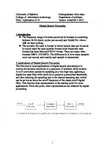
2.2. Model of Speech Production Speech production can be viewed as a filtering operation, in which a sound source excites a vocal tract filter. The source may be either periodic, resulting in voiced speech, or noisy and aperiodic, causing unvoiced speech. There are also some parts of speech which are neither voiced nor unvoiced but a mixture of the two, called the transition regions. Amplitude versus time plots of typical voiced and unvoiced speech are shown in Figure 2.1. In this speech production model the effects of the excitation source and the vocal tract are considered independently. While the source and tract interact acoustically, their independence causes only secondary effects. The voicing source occurs at the larynx at the base of the vocal tract, where the airflow from the lungs is interrupted periodically by the vocal folds generating periodic puffs of air.

8

Voiced speech Amplitude

0.5 0 −0.5 −1 0

50

100

150 200 Unvoiced speech

250

300

100 150 200 250 Time (samples, 1 sample=0.125 ms)

300

0.1 Amplitude

The rate at which the analog signal is sampled is known as the sampling frequency, Fs. The Nyquist theorem requires that Fs be greater than twice the bandwidth of the signal to avoid aliasing distortion. Thus the analog signal is low-pass filtered before sampling. As the low-pass filter is not ideal, the sampling frequency is chosen to be higher than twice the bandwidth. In telecommunication networks, the analog speech signal is bandlimited to 300-3400 Hz and sampled at 8 kHz. Hereafter, the term speech coding (see § 2.9) will refer to the coding of this type of signal. For higher quality, speech is band-limited to 0-7000 Hz and sampled at 16 kHz. The resulting signal is referred to as wideband speech. The sampled signal is quantized in amplitude via an analogto-digital converter, which represents each real sample by a number selected from a finite set of L possible amplitudes (where B = log2L is the number of bits used to digitally code the values). This quantization process adds a distortion called quantization noise, which is inversely proportional to L. In practice 12 bits are needed to guarantee an SNR higher than 35 dB over typical speech ranges [Osha87].

Digital Speech Processing

0

−0.1 0

50

Figure 2.1: Typical voiced and unvoiced speech waveforms.

The rate of this excitation is the fundamental frequency F0, also known as pitch. Voiced speech has thus a spectra consisting of harmonics of F0. Typical speech has an F0 of 80-160 Hz for males. Average F0 values for males and females are respectively 132 Hz and 223 Hz. Unvoiced speech is noisy due to the random nature of the excitation signal generated at a narrow constriction in the vocal tract. The vocal tract is the most important component in the speech production process. For both, voiced and unvoiced excitation, the vocal tract acts as a filter, amplifying certain sound frequencies while attenuating others. The vocal tract can be modeled as an acoustic tube with resonances, called formants, and antiresonances (or spectral valleys). These formants are denoted as Fi, where F1 is the formant with the lowest center frequency). The formants correspond to poles of the vocal tract frequency response, whereas some spectral nulls are due to the zeros. Moving the articulations of the vocal tract alters the shape of the acoustic tube, changing its frequency response.

9


Digital Speech Processing Voiced speech 40

Magnitude (dB)

Thus, the produced speech signal is non-stationary (timevarying) changing characteristics as the muscles of the vocal tract contract and relax. Whether or not the speech signal is voiced, its characteristics (e.g., spectral amplitudes) are often relatively fixed or quasi-stationary over short periods of time (10-30 ms), but the signal changes substantially over intervals greater than the duration of a given sound (typically 80 ms).

20 0 −20 −40 0

1000

2.3. Frequency-domain Analysis of the Speech Signal

4000

3000

4000

Magnitude (dB)

40 20 0 −20 −40 0

1000

2000 Frequency (Hz)

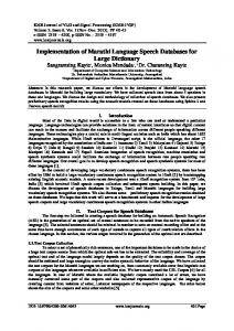
Figure 2.2: Spectra of the voiced and unvoiced speech waveforms shown in Figure 2.1, and 10-th order LPC envelope.

∞

∑ w(k − n ) ⋅ s(n) ⋅ e − jωn

n = −∞

(2.1)

Due to the non-stationary nature of speech, the signal is windowed, by multiplication with w(k − n) , to isolate a quasistationary portion for spectral analysis. The choice of duration and shape of the window w(n), as well as the degree of overlap between successive windows, reflects a compromise in time and frequency resolution. Tapered cosine windows such as the Hamming window are typically used, and the length of the window is usually 10 to 30 ms for speech sampled at 8 kHz. In Equation (2.1), the variable ω is the angular frequency, which is related to the real frequency Ω (in Hz) by the equation: ω = 2 πΩ Fs

10

3000

Unvoiced speech

Most useful parameters in speech processing are found in the spectral domain. The speech signal is more consistently and easily analyzed spectrally than in the time domain and the common model of speech production (see § 2.2) corresponds well to separate spectral models for the excitation and the vocal tract. The hearing mechanism appears to pay much more attention to spectral amplitude of speech than to phase or timing aspects (see § 2.6). For these reasons, spectral analysis is used primarily to extract relevant parameters of the speech signal. One form of spectral analysis is the short-time Fourier transform, which is defined, for the signal s(n), as: S k (e jω ) =

2000

(2.2)

Another variable which is sometimes used is the normalized frequency f, related to ω and Ω by: f = Ω Fs ,

f = ω 2π

(2.3)

As the spectrum of a digital signal is periodic in ω, the useful range for the frequency, corresponding to one period of the spectrum is given by: 0 ≤ ω ≤ 2π , 0 ≤ f ≤ 1, and 0 ≤ Ω ≤ Fs . Furthermore, as the speech signal is real, the spectrum is symmetric and the interesting frequency range is: 0 ≤ ω ≤ π , 0 ≤ f ≤ 0.5 , and 0 ≤ Ω ≤ Fs 2 . The short-time power spectra of the voiced and unvoiced speech waveforms of Figure 2.1, as well as their 10-th order LPC envelope (see § 2.4) are shown in Figure 2.2. The discrete Fourier transform (DFT) is used for computation of Equation (2.1) so that the frequency variable ω takes N discrete values (N corresponding to the window duration). Since the Fourier transform is invertible, no

11



information is lost in this representation. A more economical representation of speech parameters is achieved by the use of linear predictive analysis.

Pitch Period Impulse Train Generator

Voiced / Unvoiced Switch

LPC Coefficients

2.4. Linear Predictive Modeling of the Speech Signal

e(n)

Spectral magnitude is a relevant aspect of speech which is widely used in speech processing. One source of spectral magnitude is the short-time Fourier transform. Alternatively, linear predictive coding (LPC) provides an accurate and economical representation of the envelope of the short-time power spectrum of speech. In LPC analysis, the short-term correlation between speech samples (formants) is modeled and removed. This technique is based on the model of speech production explained in Section 2.2. A simplified block diagram of this model is shown in Figure 2.3. In this model, the excitation signal, e(n), is either an impulse train (for voiced speech) or white noise (for unvoiced speech). The combined spectral contributions of the glottal flow, the vocal tract, and the radiation of the lips are represented by a time varying digital filter. This filter is called the LPC synthesis filter. Its transfer function has both poles and zeros, but to minimize analysis complexity, the filter is assumed to be all-pole, with a transfer function given by: H p (z) =

S(z) 1 1 = = p − k E(z) 1 + ∑ a (k) ⋅ z A p (z) k =1 p

(2.4)

where {ap(1),…,ap(p)} are the LPC coefficients and p is the order of the filter (or LPC order). An order of 10 is typically used for telephone bandwidth (300-3400 Hz) speech sampled at 8 kHz. Using this LPC order, formant resonances and general spectral shape (envelope) are modeled accurately. The 10-th order LPC spectra for the voiced and unvoiced speech waveforms of Figure 2.1 (superposed to its corresponding short-time power spectra), is shown in Figure 2.2.

Time Varying Filter

s(n)

Output Speech

G

Random Noise Generator

Figure 2.3: Block diagram of the simplified source filter model of speech production.

The LPC analysis filter is given by: A p (z) = 1 + ∑ k = 1 a p (k) ⋅ z − k p

(2.5)

Transforming Equation (2.4) to the time domain results in:

e(n) = s(n) + ∑ k = 1 a p (k) ⋅ s(n − k) = s(n) − s (n) p

(2.6)

It is seen that the current speech sample s(n) is predicted by a linear combination of p past samples, s (n) . Thus the signal e(n) is the prediction error or residual signal. Hence, the p-th order LPC analysis problem is stated as follows: given measurements of the signal s(n), determine the parameters {ap(1),…,ap(p)} so as to minimize the error signal e(n).

2.5. Calculation of the LPC Coefficients Using the least-squares method, the LPC coefficients are determined by minimizing the mean energy of the error signal, given by: εp =

∞

∞

∑ e2 ( n) = ∑

−∞

−∞

[s(n) + ∑

p a ( k) ⋅ s( n − k=1 p

k)

]

2

(2.7)

The summation range is limited by windowing either the speech or the error signal, leading to the autocorrelation or covariance 12

13


method, respectively. The autocorrelation method is computationally more efficient than the covariance method and the resulting synthesis filter is always stable. In the autocorrelation method, the LPC coefficients are calculated by using the efficient Levinson-Durbin recursion (see § 5.2). This method is very popular in speech coders such as the CELP FS1016 (see § 5.11). An alternative representation of the LPC coefficients (see § 5.4), which corresponds to the multipliers of a lattice filter realization of the LPC synthesis filter, are the Parcor (partial correlation) or reflection coefficients, {k1,…,kp}. The LPC coefficients can be transformed to reflection coefficients and vice versa, using the recursions given in Equations (5.18) and (5.19). There are some LPC calculation methods, which give directly the reflection coefficients, without calculating the LPC coefficients. Two of these methods are Burg’s method [Kond94] and LeRoux-Gueguen method (see § B.1). Instantaneous (sample by sample) adaptation of the reflection coefficients is obtained by using a gradient leastmean-square (LMS) adaptive algorithm [Widr85]. In this case, the LPC calculation algorithm is called the gradient adaptive lattice (GAL) predictor. This LPC calculation algorithm is used in the noise reduction/speech enhancement algorithm for digital hearing aids described in Chapter 4.

2.6. Hearing and Speech Perception The speech signal entering the listener’s ear is converted into a linguistic message [Osha87]. The ear is especially responsive to those frequencies in the speech signal that contain the most information relevant to communication (i.e., frequencies approximately in the 200-5600 Hz range). The listener is able to discriminate small differences in time and frequency found in speech sounds within this frequency range. Key perceptual aspects of a speech signal are more evident when represented spectrally than in the time domain. Spectral amplitude is much more important than phase for speech perception and whether a sound can be heard depends on its spectral amplitude. The minimum intensity at which a sound

14


can be heard is known as the hearing threshold, which rises sharply with decreasing frequency below 1 kHz and with increasing frequency above 5 kHz. An upper limit is given by the intensity at which a sound causes discomfort or pain, known as the threshold of pain. The range between the thresholds of hearing and pain is known as the auditory field. Speech normally occupies only a portion of the auditory field. Formant frequencies and amplitudes (see § 2.2) play an important role in speech perception. Vowels are distinguished primarily by the location of their three formant frequencies, while formant transitions provide acoustic cues to the perception of consonants. Formant bandwidths are poorly discriminated and their changes appear to affect perception primarily through their effects on formant amplitudes. The valleys between formants are less perceptually important than formant peaks and humans have relatively poor perceptual resolution for spectral nulls.

2.7. Speech Processing and DSP Systems A digital signal processing (DSP) system is an electronic system applying mathematical operations to digitally represented signals such as digitized speech [Laps97]. DSP enjoys several advantages over analog signal processing. The most significant is that DSP systems are able to accomplish tasks which would be very difficult, or even impossible with analog electronics. Besides, DSP systems have other advantages over analog systems such as flexibility and programmability, greater precision, and insensitivity to component tolerances. Analog signal processing requires specific equipment, rewiring, and calibration for each new application, while digital techniques may be implemented, tested and easily modified on general purpose computers. These advantages, coupled with the rapidly increasing density of digital IC manufacturing processes make DSP the solution of choice for speech processing.

15



2.8. Digital Speech Processing Areas and Applications

2.9. Speech Coding

In the previous sections, some aspects of speech signals that are important in the communication process were described. Some areas of speech processing, such as speech coding, encryption, synthesis, recognition and enhancement, as well as speaker verification, utilize the properties of the speech signal to accomplish their goals [Rabi94], [Lim83]. In Table 2.1, typical system applications of these speech processing areas are given [Laps97]. It is seen that several of these applications are characterized by tight constraints in power consumption and size. Among them we can mention: hearing aids, digital cellular telephones, vocal pagers and portable multimedia terminals with speech i/o [Chan95].

Speech coding is the process of compressing the information in a speech signal either for economical storage or for transmission over a channel whose bandwidth is significantly smaller than that of the uncompressed signal. The ideal coder has low bit rate, high perceived quality, low signal delay, low complexity and high robustness to transmission errors. In practice, a trade-off among these factors is done, depending on the requirements of the application. The term speech coding (or narrowband speech coding) refers to the coding of telephone bandwidth (300-3400 Hz) speech sampled at 8 kHz, whereas the term wideband speech coding refers to the coding of speech band-limited to 0-7000 Hz and sampled at 16 kHz. The speech research community has given different names to different qualities of speech found in a telecommunication network [Osha87]:

Digital speech processing area Speech coding and decoding Speech encryption and decryption Speech recognition

Speech synthesis Speaker verification Speech enhancement (e.g., noise reduction, echo cancellation, equalization) Table 2.1:

16

System applications

Digital cellular telephones, digital cordless telephones, vocal pager, multimedia computers and terminals, secure communications. Digital cellular telephones, digital cordless telephones, multimedia computers and terminals, secure communications. Advanced user interfaces, multimedia computers and terminals, robotics, automotive, digital cellular telephones, digital cordless telephones. Multimedia computers, advanced user interfaces, robotics. Security, multimedia computers, advanced user interfaces. Hearing aids, hands-free telephone, telephone switches, automotive, digital cellular telephones, industrial applications.

Typical system applications of different speech processing areas.

(1) Toll quality describes speech as heard over the switched telephone network. The frequency range is 300-3400 Hz, with signal-to-noise ratio of more than 30 dB and less than 2-3 % of harmonic distortion. (2) Communications quality speech is highly intelligible but has noticeable distortion compared with toll quality. (3) Synthetic quality speech is 80-90 % intelligible but has substantial degradation, sounding “buzzy” or “machinelike” and suffering from lack of speaker identifiability. Some nuances in this characterization are found in speech research, where sometimes a coder is described as having “near toll quality”, or “good communications quality”. The bit rate of a coder is expressed in bits per seconds (bps) or kilobits per second (kbps) and is given by: Tc (kbps) = B (No. of bits) ⋅ Fs (kHz)

(2.8)

Toll quality corresponds to (300-3400 Hz) band-limited speech sampled at 8 kHz and represented with 12 bits (uniform quantization). The bit rate is thus 96 kbps. Using µ-law or A-law logarithmic compression, the number of bits is reduced to 8, and

17


thus the bit rate to 64 kbps. This logarithmic coding was standardized as the ITU-T G.711 and is used as a reference for toll quality in speech coding research. In communications systems such as satellite communications, digital mobile radio, and private networks, the bandwidth and power available are severely restricted, hence reduction of the bit rate is vital. This is done at the expense of decreased quality and higher complexity. Toll quality is found in coders ranging from 64 kbps to 10 kbps, near toll and good communications quality is found in the range of 10 to 2.4 kbps, and communications to synthetic quality below 4.0 kbps.

Vector Quantization Vector quantization (VQ) is the process of quantizing a set of k values jointly as a single vector. If the vector elements are correlated, the number of bits to represent them is reduced with respect to scalar quantization. The block diagram of a simple vector quantizer is shown in Figure 2.4. The codebook Y contains a number L of codevectors yi of dimension N: yi = [yi1, yi2, …, yiN]T. The subindex i is the address or index of the codevector yi . Each codevector is uniquely represented by its index. The length of the codebook L, and the number of bits of the index B are related by: B = log2L. The N dimensional input vector x = [x1, x2, …, xN]T is vector quantized by first finding its “closest” vector in the codebook, and then representing x by the index of this closest vector. The closest vector is the one that minimizes some distortion measure. Typical distortion measures are the mean squared error and the weighted mean squared error. The codebook design process is known as training or populating the codebook. One popular method for codebook design is the k-means algorithm [Kond94]. The number of codevectors L, should be large enough that for each possible input vector, substitution by its closest codevector does not introduce excessive error. However, L must be limited to limit the computational complexity of the search and because the bit rate is proportional to B = log2L.

18


x(n)

Input Vector Buffer

x

Vector Matching

index i

yi Codebook Y Figure 2.4: Block diagram of a simple vector quantizer.

The main drawback of vector quantization is its high computational and storage cost. Compared to scalar quantization, the major additional complexity of VQ lies in the codebook search. In a full codebook search, the input vector is compared with each of the L vectors of the codebook, requiring L computationally expensive distance calculations. The codebook size is also a problem for codebook training. As an example, if a 20-bit representation is needed, the codebook should contain 220 codevectors of dimension N. This would require a prohibitively large amount of training data, and the training process would need too much time. Besides, as the codebook is stored at both the receiver and the transmitter, the storage requirement would be prohibitively high. Practical VQ systems use suboptimal search techniques that reduce search time and sometimes codebook memory while sacrificing performance. Among these techniques there are treesearched VQ, multistage VQ, classified VQ and split VQ [Gers94]. In CELP coders, VQ is used for quantization of the excitation signal, and sometimes also to model the long term correlation of the speech signal (pitch) by means of an adaptive codebook search. Additionally, VQ is successfully used to quantize spectral parameters (i.e., any representation of the LPC coefficients) as explained in Section 5.8.

19



CELP coding Most notable and most popular for speech coding is code excited linear prediction (CELP). These coders had a great impact in the field of speech coding and had found their way in several regional and international standards. While newer coding techniques have been developed, none clearly outperforms CELP in the range of bit rates from 4 to 16 kbps [CELP97]. The obtained quality ranges from toll to good communications quality. Furthermore, several reduced complexity methods for CELP were studied in speech coding research. As a result, more than one full-duplex CELP coder can nowadays be implemented on a state-of-the-art DSP processor. Current research goes in the direction of reducing complexity and enhancing performance. Another current trend is the use of speech classification, notably voice activity detection (VAD) and voice/non voice classification for bit rate reduction. The obtained coders are variable bit rate coders, with an average bit rate lower than 3 kbps and the same quality of fixed rate coders at 4.8 kbps. CELP coding refers to a family of speech coding algorithms which combine LPC-based analysis-by-synthesis (AbS-LPC) and vector quantization (VQ) [Gers94]. The general diagram of a CELP coder is shown in Figure 2.5. In AbS-LPC systems, the LPC model is used (see § 2.4), in which an excitation signal, e(n), is input to a synthesis filter, Hp(z), to yield the synthetic speech output s( n ) . There are two synthesis filters. The LPC synthesis filter models the short-term correlation between speech samples (formants) whereas the pitch synthesis filter models the longterm correlation (pitch). The coefficients of the LPC synthesis filter are determined from a frame of the speech signal, using an open-loop technique such as the autocorrelation method (see § 2.5). The coefficients of the pitch synthesis filter are also determined by open loop techniques [Kond94].

20

γ

Stochastic Codebook

Pitch Synthesis Filter

Original Speech Signal Instantaneous LPC Synthesis Objective Filter Error

Long Term Predictor

Short Term Predictor

Minimize Perceptual Error

Perceptual Weighting Filter

Figure 2.5: Block diagram of a general CELP coder.

Once the parameters of the LPC and pitch synthesis filters are determined, an appropriate excitation signal is found by a closed-loop search. The input of the synthesis filters is varied systematically, to find the excitation signal that produces the synthesized output that best matches the speech signal, from a perceptual point of view. Vector quantization (VQ) is combined with AbS-LPC in CELP coders [Gers94]. The optimum excitation signal is selected from a stochastic codebook of possible excitation signals (codevectors). Each codevector is passed through the LPC and pitch synthesis filters. The codevector which produces the output that best matches the speech signal is selected. In some CELP coders, such as the FS1016 (see § 5.11) the pitch synthesis filter is substituted by a search on an adaptive codebook, which models long term correlation.

Parametric Coders Fixed rate CELP coders do not perform well with bit rates below 4 kbps. Using parametric coders [LOWB97], good communications and near toll quality is obtained at 2.4 kbps. These speech coders are based on algorithmic approaches such as sinusoidal coders, in particular sinusoidal transform coding (STC) and multiband excitation (MBE). Another widely used approach is prototype waveform interpolation (PWI), which is a

21


technique to efficiently model voiced excitation. Combining parametric coders with frame classification schemes, variable bit rate coders with average bit rate of 1.3 kbps are obtained. The main disadvantage of parametric coders is their high complexity, and lower quality when compared with CELP coders.

2.10. Speech Enhancement Speech enhancement involves processing speech signals for human listening or as preparation for further processing before listening [Lim83]. The main objective of speech enhancement is to improve one or more perceptual aspects of speech, such as overall quality or intelligibility. Speech enhancement is desirable in a variety of contexts. For example, in environments in which interfering background noise (e.g., office, streets and motor vehicles) results in degradation of quality and intelligibility of speech. Other applications of speech enhancement include correcting for room reverberation, correcting for the distortion of speech due to pathological difficulties of the speaker, postfiltering to improve quality of speech coders, and improvement of normal undegraded speech for hearing impaired people. An example of speech enhancement is the algorithm described in Chapter 4, which was studied and optimized for implementation. In this algorithm, spectral sharpening is used for both noise reduction and to compensate for the loss in frequency selectivity encountered among hearing impaired people.

Digital Hearing Aids Analog electroacoustic hearing aids are the primary treatment for most people with a moderate-to-severe sensorineural hearing impairment [Work91]. These conventional hearing aids contain the basic functions of amplification, frequency shaping, and limiting of the speech signal. The conventional hearing aids provide different amounts of amplification at different

22


frequencies so as to fit as much of the speech signal as possible in the reduced auditory field (see § 2.6) of the hearing impaired person. Digital hearing aids promise many advantages over conventional analog hearing aids. The first advantage is the increased precision and programmability in the realization of the basic functions. The frequency response can be tailored to the needs of the patient and also change according to different acoustic situations. Another advantage is the possibility of adding new functions such as noise reduction, spectral sharpening and feedback cancellation, which are impossible or very difficult using analog circuits. Furthermore, external computers can be used to simulate and study new algorithms to be included in the hearing aid and for new and improved methods of prescriptive fitting and evaluation. On the other hand, the physical implementation of digital hearing aids is characterized by very tight requirements [Lunn91]: (1) Size: the small physical dimensions of analog hearing aids contribute to the acceptance by the user. The smallest devices (in-the-channel hearing aids) have just some cm3 to accommodate microphone, receiver, signal processing chip and power supply. (2) Power supply: for keeping a small dimension, only one 1.5 battery cell should be used. (3) Power consumption: typical values of 1-2 mW, to allow a battery life of several weeks. These requirements are very difficult to fulfill given the complexity and number of functions to be implemented, the real time requirement and the large dynamic range of the input signals. Therefore, the physical implementation of digital hearing aids can only be achieved by a careful optimization that ranges from algorithm level, through system and circuit architecture to layout and design of the cell library. In Chapter 4, the optimization of the implementation of a noise reduction/speech enhancement algorithm for digital hearing aids is presented.

23


The sampling frequency for digital hearing aids is a controversial issue. In [Lunn91] an Fs of 12 kHz is used, whereas in several algorithms proposed in literature, an F s of 8 kHz is used. Higher sampling rates may be unnecessary due to the reduced auditory field of the hearing impaired person.

2.11. Speech Processing Functional Blocks Some functional blocks which are typically used in the different speech processing areas, and which were optimized for implementation in the work described in this report, are explained as follows.

Lattice FIR, IIR and GAL Predictor Lattice filters and lattice linear predictors are used in many areas of digital speech processing such as coding, synthesis and recognition, as well as in the implementation of adaptive filters [Proa89], [Osha87]. The lattice structure offers significant advantages over the transversal filter realization. The lattice filter performance using finite word-length implementation is much superior to that exhibited by the direct implementation. Also, the lattice adaptive linear predictor presents faster convergence than the direct form when the stochastic gradient algorithm (LMS) is used [Honi88]. In commercial speech synthesis chips the lattice filter is prevalently used because of its guaranteed stability and suitability for fixed-point arithmetic [Osha87], [Wigg78], [Iked84]. Furthermore, lattice filter structures are particularly suitable for VLSI implementation due to their modular structure, local interconnections, and rhythmic data flow [Kail85]. The noise reduction/speech enhancement algorithm described and optimized in Chapter 4 is based on lattice filter structures (GAL LPC predictor, and modified FIR and IIR lattice filters). These functional blocks find also application in other speech processing systems (see § 4.8). The GAL predictor is used in backward predictive speech coders and other systems where instantaneous update of spectral information is needed.

24


The modified FIR and IIR filters studied in Chapter 4 are the basis for the postfiltering algorithm found in several speech coders and vocoders to improve quality of the synthesized speech. These modified FIR and IIR filters are also used in CELP coders for perceptual weighting of the error between the original and synthesized speech. Finally the IIR lattice filter is ideal for the implementation of the LPC synthesis filter found in most speech coding and synthesis systems.

LPC Calculation LPC provides an accurate and economic representation of the speech spectral envelope (see § 2.4). This representation is used in speech coding to model and remove short-term correlation of the input signal. The LPC coefficients are used in the synthesis filter found in speech synthesis systems. Due to its representation of perceptually important speech parameters it is also used in speech recognition and speaker verification systems. An interesting aspect of LPC analysis is that it is not just applied to speech processing, but also to a wide range of other fields such as control and radar [Osha87]. Two types of LPC calculation algorithms were optimized for implementation in the work described in this report. One is the LPC calculation on a frame-by-frame basis using the autocorrelation method and the Levinson-Durbin recursion. This algorithm was optimized for implementation on a fixed-point commercial DSP as part of the DSP56001 implementation of the CELP FS1016 spectral analysis and quantization described in Chapter 7. The second is the sampleby-sample calculation of the reflection coefficients done with the GAL predictor, which was optimized for both implementation on a DSP56001 and on a low power VLSI architecture, as described in Chapter 4.

25



LSP Representation of LPC Parameters

Real-time Constraints

Line spectrum pair (LSP) parameters are a one to one representation of the LPC coefficients. This representation allows more efficient encoding (quantization) of spectral information, and is very popular in low bit rate coding (see § 5.6, 5.7 and 5.8). LSP parameters are not only used to encode speech spectral information more efficiently than using other representations, but also provide good performance in speech recognition [Pali88], and speaker recognition [Liu90]. On the other hand, the calculation of LSP parameters from LPC coefficients is a computationally intensive task, as it involves the resolution of polynomials by numerical root search. In Chapter 5, a survey of existing algorithms for LSP calculation is given (see § 5.9). Three algorithms which are found promising for efficient real time implementation are retained for further study and comparison. In Chapter 6, two new efficient algorithms for LSP calculation are presented, and then compared with existing algorithms from the point of view of accuracy, reliability and computational complexity. The efficient implementation of these algorithms on a DSP56001 is given in Chapter 7. Efficient implementation of LSP to LPC conversion is also addressed in Chapter 5, 6, and 7.

A real-time process is a task which needs to be performed within a specified time limit. Most speech processing systems must meet rigorous speed goals, since they operate on segments of real-word signals in real-time. While some systems (like databases) are required to meet performance goals on average, speech processing algorithms must meet goals at defined instants of time. In such systems, failure to maintain the necessary processing rates is considered a serious malfunction. These systems are said to be subject to hard real-time constraints. In digital speech processing, the processing needs to be performed within 125 µs for sample-by-sample processes (with Fs = 8 kHz). The allowed time is higher for processes performed on a frame-by-frame basis, such as LPC calculation with autocorrelation method (see § 2.5), with typical block lengths of 20-30 ms, and subframe lengths of 5-10 ms.

2.12. Implementation Issues The goal of speech coding is reducing bit rate, without degrading speech quality, whereas hearing aids are aimed to improve speech intelligibility and perceived quality. However, in the implementation of these algorithms, other factors apart from the their functionality are of importance. Some of these factors are discussed as follows.

26

Processing Delay In some speech processing applications, such as digital hearing aids and telecommunications, the total delay has to be kept within specified limits. The processing time usually adds to other components of the total delay (e.g., algorithmic delay and transmission delay). Thus, in some cases the processing speed has to be increased beyond the speed required for real-time operation, to keep up with the delay requirement.

Programmable DSP versus Custom Hardware The designer needs to decide whether to use a programmable DSP chip or to build custom hardware. These two options are discussed next.

27



Programmable DSP Implementation

Custom Hardware and ASIC

Programmable digital signal processors (often called DSPs) are microprocessors that are specialized to support the repetitive, numerically intensive tasks found in DSP processing [Laps97]. Dozen of families of DSPs are available on the market today. The first task in selecting a DSP processor is to weight the relative importance of performance, cost, integration, ease and cost of development, and size and power consumption for the desired application. Algorithmic optimization is very important from the cost point of view. Any speech processing algorithm can be implemented using commercially available DSP processors, but the cost will increase rapidly with the number of DSP chips used. Another important consideration is the power consumption of the final product, especially if it is a portable, battery operated device. A key issue is the choice of a fixed-point or floating-point device. Floating-point DSPs are costlier and have a higher power consumption than fixed-point DSPs. Floating-point operations require more complex circuitry and larger word sizes (which imply wider buses and memory) increasing chip cost. Also, the wider off-chip buses and memories required increase the overall system cost and power consumption. On the other hand, floating-point DSPs are easier to program, as, usually, the programmer does not have to be concerned by dynamic range and precision considerations. Most high volume applications use fixed-point processors because the priority is low cost. For applications that are less cost sensitive, or that have extremely demanding dynamic range and precision requirements, or were ease of programming is important, floating-point processors are the choice. Note also that the implementation on a commercial fixed-point DSP can be seen as an intermediate step before the actual implementation using custom hardware (see § 4.4 and 4.6). This implementation allows real time evaluation, optimization of the scheduling, and helps in the study and optimization of the fixed-point behavior.

There are two important reasons why custom-developed hardware is sometimes a better choice than a commercial DSP implementation: performance and production cost. In virtually any application, custom hardware can be designed which provides a better performance than a programmable DSP. Furthermore, in some applications such as digital hearing aids, the tight constraints in size and power can only be met by using custom hardware. For high volume products, custom hardware is less expensive than a DSP processor. Due to its specialized nature, custom hardware has the potential to be more cost effective than commercial DSP chips. This is because a custom implementation places in the hardware only those functions needed by the application, whereas a DSP processor requires every application to pay for the full functionality of the processor, even if it uses only a small subset of its capabilities. Custom hardware can take many forms, such as printed circuit boards using off-the shelf components, but this form is falling out of favor as the performance of DSP processors increases. In case a very high performance is needed, or very low power and size are required, the solution is the use of application specific integrated circuits (ASIC). Designing a custom chip provides the ultimate flexibility, since the chip can be tailored to the needs of the application. On the other hand, the development cost is high, and the development time can be long. A key point for an optimized ASIC DSP implementation is the choice of a fixed-point arithmetic, and minimization of the number of bits needed for the representation of constants and variables (see § 3.1).

28

2.13. Fixed-point versus Floating-point Arithmetic The choice of a fixed-point arithmetic is a key point to decrease cost, size, and power consumption in both programmable DSP and ASIC implementations. As in speech processing applications such as hearing aids and portable communications devices,

29



minimization of cost, size, and power consumption is essential, a fixed-point arithmetic is chosen. This implies a higher development effort. The designer has to determine the dynamic range and precision needs of the algorithms before implementation, either analytically, or through simulation.

In Chapter 3, a methodology for optimization of speech processing algorithms is presented. The emphasis is placed in algorithmic optimization and the study of fixed-point quantization effects.

2.16. References 2.14. Algorithmic Optimization [CELP97]

ICASSP’97 session: "CELP Coding", 12 different papers, Proc. IEEE Int. Conf. on Acoustics, Speech, and Signal Processing, ICASSP’97, Vol.2, pp. 731-778, 1997.

[Chan95]

A. Chandrakasan and R. Brodersen, “Minimizing Power Consumption in Digital CMOS Circuits”, Proc. of the IEEE, Vol. 83, No. 4, pp. 498-523, 1995.

[Gers94]

A. Gersho, “Advances in Speech and Audio Compression”, Proc. of the IEEE, Vol. 82, No. 6, 1994.

[Honi88]

M. Honig and D. Messerschmitt, Adaptive Filters: Structures, Algorithms, and Applications, Kluwer Academic Publisher, Boston, USA, 1988.

[Iked84]

O. Ikeda, "Speech Synthesis LSI LC8100", Proc. of Speech Technology, New York, pp. 188-191, 1984.

[Kail85]

T. Kailath, "Signal Processing in the VLSI Era" in VLSI and Modern Signal Processing, ed. by S. Kung, H. Whitehouse, and T. Kailath, Prentice Hall, Englewood Cliffs, NJ, 1985.

[Kond94]

A. M. Kondoz, Digital Speech: Coding for Low Bit Rate Communication Systems (Chapter 3, 11), Wiley, Chichester, 1994.

[Laps97]

P. Lapsley et al., DSP Processor Fundamentals: Architectures and Features, IEEE Press Series on Signal Processing, Piscataway, NJ, 1997.

[Lim83]

J. Lim (Editor), Speech Enhancement, Prentice-Hall Signal Processing Series, Englewood Cliffs, New Jersey, 1983.

2.15. Summary of the Chapter

[Liu90]

In this chapter a brief introduction to the field of digital speech processing and its applications was given. It was shown that algorithmic optimization and the choice of a fixed-point arithmetic are essential in speech processing applications such as hearing aids or portable communications devices.

Chi-Shi Liu et al., "A Study of Line Spectrum Pair Frequencies for Speaker Recognition", Proc. IEEE Int. Conf. on Acoustics, Speech, and Signal Processing, ICASSP'90, Vol. 1, pp. 277-280, 1990.

[LOWB97]

ICASSP’97 session: "Speech Coding at Low Bit Rates", 14 different papers, Proc. IEEE Int. Conf. on Acoustics, Speech, and Signal Processing, ICASSP'97, Vol.2, pp. 1555-1610, 1997.

Algorithmic optimization is essential to obtain a low power ASIC implementation. This is seen in Table 2.2, where the expected power saving at different implementation levels is given [Raba97]. An explanation of all the possible optimization strategies listed in this table is out of the scope of this report. Implementation level

Optimization strategy

Expected saving

Algorithm Behavioral Power Management Register Transfer Level Technology independent Technology dependent

Algorithmic selection Concurrency memory Clock control Structural transformation Extraction/ decomposition Technology mapping Gate sizing Placement

Orders of magnitude Several times 10-90% 10-15%

Layout Table 2.2:

30

15% 20% 20%

Expected power saving by optimization carried out at different implementation levels.

31

Optimized Implementation of Speech Processing Algorithms [Lunn91]

T. Lunner and J. Hellgren, "A Digital Filterbank Hearing Aid Design, Implementation and Evaluation", Proc. IEEE Int. Conf. on Acoustics, Speech, and Signal Processing, ICASSP'91, Vol. 5, pp. 3661-3664, 1991.

[Neuv93]

Y. Neuvo, "Digital Filter Implementation Considerations" in Handbook for Digital Signal Processing, ed. by S. Mitra and J. Kaiser, Wiley, New York, 1993.

[Osha87]

D. O'Shaughnessy, Speech Communication: Human and Machine (Chapter 3, 4, 5, 6 and 7), Addison-Wesley, Reading, 1987.

[Pali88]

K. Paliwal, "A Study of Line Spectrum Frequencies for Speech Recognition", Proc. IEEE Int. Conf. on Acoustics, Speech, and Signal Processing, ICASSP'88, Vol. 1, pp. 485488, 1988.

[Proa89]

J. Proakis and D. Manolakis, Introduction to Digital Signal Processing, Macmillan, New York, 1989.

[Raba97]

J. Rabaey, Cad Tools for Low Power, Electronics Laboratories Advanced Engineering Course on: Architectural and Circuit Design for Portable Electronic Systems, EPFL, Lausanne, 1997.

[Rabi94]

L. Rabiner, “Applications of Voice Processing to Telecommunications”, Proc. of the IEEE, Vol. 82, No. 2, pp. 199-228, 1994.

[Thon93]

T. Thong and Y. Jenq, "Hardware and Architecture" in Handbook for Digital Signal Processing, ed. by S. Mitra and J. Kaiser, Wiley, New York, 1993.

[Widr85]

B. Widrow and S. Stearns, Adaptive Signal Processing, Prentice-Hall, Englewood Cliffs - N.J, 1985.

[Wigg78]

R. Wiggins and L. Brantingham, "Three Chip System Synthesizes Human Speech", Electronics, Vol. 51, No. 18, pp. 109-116, 1978.

[Work91]

32

Working-group on Communication and Aids for the Hearingimpaired People, "Speech-perception Aids for Hearingimpaired People: Current Status and Needed Research", J. of the Acoustical Society of America, Vol. 90, No.2, pp. 637-685, 1991.

Chapter 3 Methodology of Optimization In this chapter, a methodology for optimization of speech processing algorithms is presented. The emphasis is placed in algorithmic optimization (algorithm choice and simplification) and the study of fixed-point quantization effects. A practical method for evaluating the behavior of digital signal processing (DSP) algorithms in the case of an implementation using fixed-point 2's complement arithmetic is proposed. A theoretical study of quantization effects is out of the scope of this report and can be found among others in [Jack89] and [Vaid87].

3.1. Methodology of Optimization Some speech processing applications such as digital hearing aids and portable telecommunications devices, are characterized by very tight requirements in chip size and power consumption as well as the complexity and number of functions to be implemented. The proposed methodology of optimization (Figure 3.1) is aimed to efficient implementation of these devices. A good interrelation between algorithmic level and target architecture is essential in this optimization process. The system is simulated using a double-precision C program. This program is first used to evaluate the performance

33

34

Figure 3.1: Methodology for algorithmic optimization.

Target Architecture High Level Specification

3.2. Quantization Effects in Digital Signal Processing Finite-precision effects are inherent of any digital realization whether it be hardware or software. There are two common forms to represent numbers in a digital computer, fixed-point and floating-point notation. In practice fixed-point implementation leads to more efficient solutions on custom hardware, in terms of area and power consumption. Also, most popular low-cost commercial DSP chips are based on fixed-point arithmetic. Floating-point arithmetic is briefly described in [Proa89] and [Vaid87]. Hereafter, only fixed-point representation is considered.

Fixed-point Optimization

Algorithmic Modification

Low Power, Small Area,VLSI Implementation Algorithmic Choice

Algorithmic Study

of the system and to tune its parameters and then is used as reference system for further optimization and simplification. For each functional block of the system, a survey of different algorithmic options for its realization is done. Only algorithms that are promising for efficient implementation are chosen, taking into account computational complexity, influence on the performance of the whole system, and the suitability for a fixedpoint implementation. These algorithms are modified to reduce computational complexity, improve overall performance, allow better implementation on the target architecture, or improve their fixed-point implementation. A simulation of fixed-point quantization effects is done to minimize the number of bits required at every node of the algorithm while keeping a good performance. Implementation on a commercial low-cost fixed-point DSP, such as the DSP56001 is done for real time evaluation and to observe which blocks are computationally more expensive. Custom VLSI is done using either standard cell approach and automatic CAD tools or the low power architecture and the tool for optimal scheduling of DSP algorithms proposed in [Heub94]. An example of the application of this methodology in the optimal implementation of a noise reduction/ speech enhancement algorithm for digital hearing aids is given in Chapter 4.

Methodology of Optimization

Real Time, Fixed-point DSP Implementation on DSP56001


35



3.3. Binary Fixed-point Representation of Numbers A binary representation of a number is a means of writing the number in terms of powers of two. For example the decimal number 6.375 can be represented as 110.011 , an abbreviation for: 1 ⋅ 2 2 + 1 ⋅ 2 1 + 0 ⋅ 2 0 + 0 ⋅ 2 –1 + 1 ⋅ 2 –2 + 1 ⋅ 2 –3 . A binary number comes with a "binary point". The portion to the left represents an integer (e.g., 110 = 6 ) and the portion to the right represents fractions less than one (e.g., 0.011 = 0.375 ). In fixed-point notation the binary point is constrained to lie at a fixed position in the bit pattern, as shown in Figure 3.2.

2NI-1 a NI-1

...

21 a 1

sign bit NI bits for integer

20 a 0

2-1 a -1

...

2-NF a -NF

least significant bit NF bits for fraction ai = 0,1 binary point

x = −a NI − 1 ⋅ 2 NI − 1 +

NI − 2

∑ ak ⋅ 2k

k = – NF

(3.2)

The negative of a number is obtained by subtracting the corresponding positive number from 2 NI . In the case of pure fractional arithmetic (NI=1) a negative number is obtained by subtracting its positive number from 2 (from there the name of 2's complement). The 1's complement representation is identical to signmagnitude and 2's complement for positive numbers. A negative number is formed by complementing its corresponding positive number representation. Note that zero is now represented by 000 or 111, which is an undesired ambiguity. Two's complement arithmetic is easy to implement for both additions and multiplications, and elegantly handles negative numbers. In the work described in this report, only the case of two's complement fixed-point arithmetic is studied.

Figure 3.2: Allocation of bits in a word for fixed-point implementation.

3.4. Rounding and Truncation

The first bit to the left is called the sign bit. The precision of the number system is defined as the increment between two consecutive numbers and is determined by the value of the least significant bit (LSB). Within the subclass of fixed-point representations, there are three commonly used methods to represent bipolar numbers: sign-magnitude, one's complement, and two's complement representation [Vaid87]. They are all based on the natural binary code, but differ in the way they handle negative numbers. In the sign-magnitude representation, the term:

In performing fixed-point computations such as multiplications it is often necessary to quantize a binary fixed-point number x, to another number Q[x], reducing the precision (number of fractional bits) from NF1 to NF2 as shown in Figure 3.3. This can be done via truncation or rounding. The effect of this reduction of precision is to introduce an error whose power depends on the values of NF1 and NF2 and whose statistical behavior depends on the type of truncation or rounding used. This error is referred to by the generic name of round-off error (whether rounding or truncation is actually employed) and is given by:

NI − 2

∑ a k ⋅ 2k

k = − NF

(3.1)

e = Q[ x ] − x

(3.3)

always represents the magnitude and the sign is kept in the sign bit. In the 2's complement notation a positive number is the same as in sign-magnitude representation, and a negative number is given by:

36

37


2NI-1

21

20

2-1

X

a NI-1

...

a 1

a 0

a -1

2-NF2 ...

a -NF2

Q[x]

a’ NI-1

...

a’ 1

a’ 0

a’ -1

...

a’ -NF2


2-NF1 ...

statistical behavior of the error for rounding and truncation is given in Figure 3.4.

a -NF1

Convergent Rounding

Figure 3.3: Truncation or rounding of a fixed-point binary number.

Regardless of the actual binary representation used, several types of rounding or truncation can be implemented, among them, 2's complement truncation, sign-magnitude truncation, rounding and convergent rounding.

The conventional rounding rounds up any value above one-half and rounds down any value below one-half. The question arises as to which way one-half should be rounded. If it is always rounded one way, the result will eventually be biased in one direction. Convergent rounding solves the problem by rounding down if the number is odd and rounding up if the number is even.

Truncation In truncation, the least significant bits (NF2 to NF1) are simply dropped, regardless of the sign and the convention to represent negative numbers. If x is positive then: –( 2 − NF 2 − 2 − NF 1) ≤ e ≤ 0

(3.4)

If x is negative the error depends on which binary representation is used: Sign-magnitude truncation and 1's complement truncation:

0 ≤ e ≤ (2 − NF 2 − 2 − NF 1)

and

Q[x] ≤ x

(3.5)

2's complement truncation:

−(2 − NF2 − 2 − NF1 ) ≤ e ≤ 0,

and

Q[x] ≥ x

(3.6)

Rounding In rounding, the value Q[x] is taken to be the nearest possible number to x, thus the error is limited by: −

(2 − NF2 − 2 − NF1 ) (2 − NF 2 − 2 − NF 1) ≤e≤ 2 2

(3.7)

Rounding is more accurate than truncation but requires more effort in its implementation. The quantization curve and 38

3.5. Dynamic Range, Arithmetic

Overflow,

and

Saturation

In general, a fixed-point DSP implementation is an elaborated interconnection of multipliers, adders and delays in which all the signals involved (including inputs, outputs and internal signals) are represented with fixed-point arithmetic. An overflow occurs when the value of a signal exceeds the dynamic range available. The dynamic range is the range of numbers which can be represented within the arithmetic used. In 2's complement fixed-point arithmetic, this range is given by ( MIN = −2 NI − 1 , MAX = 2 NI − 1 − 2 − NF ). Scaling is the process of readjusting some internal gain parameters to avoid overflows. In [Jack89] it is shown how scaling should be performed, depending on the class of inputs. For a fixed total number of bits there is a trade-off between decreasing the probability of overflows by scaling and increasing the round-off error. Therefore scaling is usually applied only to minimize the probability of overflow to a reasonable extent and not to preclude it entirely. When an overflow actually occurs the resulting distortion is minimized by using clipping or saturation arithmetic. The overflowed result is substituted by the values MIN or MAX, according to its sign.

39

Optimized Implementation of Speech Processing Algorithms Q[x]

Q[x]

Q[x]

x

Parameter Quantization

x

x

e = Q[x] - x

e = Q[x] - x

e = Q[x] - x

x

x

x Sign-magnitude and 1's complement truncation

2's complement truncation

Rounding


The filter coefficients are only quantized once (in the design process) and those values remain constant in the filter implementation. The effect of coefficient quantization is to deviate the filter response from its ideal (designed) form in a deterministic manner. The quantized design can be checked and, if no longer meets the specifications, can be optimized, redesigned, restructured, and/or more bit could be allocated to satisfy the specifications. The structure of the digital filter network influences directly its sensitivity to coefficient quantization.

Signal Quantization P(e)

P(e)

1/q

P(e)

1/q 1/(2q)

-q/2

q/2

σ2 = q2 / 12 E=0

e

e

-q σ2 = q2 / 12 E = -q/2

-q

q

e

σ2 = q2 / 3 E=0

Figure 3.4: Quantization curve, error and statistical behavior of the error (P(e) = pdf, E = mean, σ2= variance and q = 2–NF2–2–NF1).

3.6. Fixed-point Quantization Effects The implementation of a DSP algorithm using fixed-point arithmetic involves quantization of the signals and parameters of the system. As a result, the overall input-output behavior is not ideal. Quantization is the process of transforming a value into its closest representation in the number system by means of truncation or rounding, and clipping [Jack89]. Two basic types of quantization effects should be distinguished. The first is due to parameter quantization, where the term parameter refers to the fixed values in the algorithm, usually filter coefficients. The second is due to quantization of the input, output and internal signals of the system.

40

The effect of signal quantization is to add an error or noise signal e(n) to the ideal output y(n) of the digital filter. This noise is a composite of the errors from one or more of the following sources, as applicable: (1) The quantization error of the analog-to-digital converter at the filter input. (2) The accumulated errors resulting from truncation within the filter (round-off noise).

rounding

or

(3) The quantization of the output y(n) to fewer bits for input to a digital-to-analog converter or to another digital system. Source (3) is sometimes overlooked, but because of the accumulation of the noise in (2), more bits are usually allocated to the internal arithmetic of the filter than are required at the output. Hence, the output is usually requantized to fewer bits. It is often reasonable for the input and output quantization to employ the same number of bits, in which case their power noise levels are the same.

41


3.7. Round-off Noise and Limit Cycles The internal signals in a digital filter are invariably subject to quantization causing errors in the computed output. Such quantization is a non-linear phenomenon and can be further subdivided into two types of effects called limit-cycles and round-off noise. Round-off noise affects the filter output in the form of a random disturbance, and can be analyzed by suitable noise modeling and by the use of linear system theory [Jack89]. Limit-cycle oscillations, which contribute to undesirable periodic components at the filter output are due to the fact that quantization is a non linear operation. When such nonlinearities exist in a feedback path, they can lead to oscillations [Jack89]. In the case of a zero or constant input, ideally the output of a stable discrete-time filter would asymptotically approach zero or a constant. However, with quantization, it is often found that relatively small limit-cycle oscillations occur. A different limit-cycle mode, called rolling-pin limit-cycle, has larger amplitude and is rarely encountered [Jack89]. This rolling-pin limit cycles cannot be predicted theoretically and their occurrence is better checked by simulation. Usually, limit cycles can be reduced to acceptable levels by giving a sufficient number of bits to the signal representation. Another possible type of oscillation, due to overflows, is avoided by using saturation arithmetic.

3.8. Adaptive and Non-linear Algorithms Adaptive filters are extensively used in signal processing applications. The least-mean-square (LMS) algorithm is the most attractive adaptation scheme because of its computational simplicity. Adaptive algorithms are non-linear in nature, therefore a theoretical analysis of their finite-precision behavior is very difficult and can be performed only under very simplified conditions [Frie92], [Cara84], assuming a stationary input. The well-known theory of finite precision filters with fixed coefficients is inapplicable for adaptive filters.

42


For instance the representation of coefficients in adaptive filters requires a much longer word-length than in fixed filters. In the case of an adaptive or non-linear algorithm with nonstationary input such as speech, theoretical analysis becomes untractable. Nevertheless the practical issue of how many bits are required for proper functioning on a fixed-point implementation remains. In this case the only solution is to perform simulations of the quantized algorithms under final working conditions with the appropriate input signals.

3.9. Simulation Algorithms

of

Quantization

Effects

in

DSP

In the study by simulation of finite word-length effects on a DSP algorithm the main goal is to determine the minimum number of integer and fractional bits (NI,NF) required at every node of the algorithm, keeping the degradation of performance due to quantization effects within acceptable levels. Additionally, this study can also include optimization and modification of the algorithm to simplify its implementation on the target architecture and to improve the use of the dynamic range available.

The Environment Used The functional blocks of the DSP algorithm are coded in C language, as Matlab functions, and interfaced under Matlab [MATL93]. Inputs and outputs of a Matlab function are matrices, vectors or scalars. When coding a particular functional block, any value that the designer may wish to modify iteratively is set as input while internal variables of particular interest are returned together with the output signals of the functional block. Different functions were written to allow speech playback, to load a speech file with two different formats, and to run a program on a DSP56001 card from Matlab. The calling syntax and description of this functions is given in Table 3.1.

43


Within Matlab, the algorithms can be run with different input parameters and the signals involved can be analyzed, displayed and listened to have an immediate feed-back after introducing any change in the system. da (x, Fs)

[x, Fs] = rd_timit ('filename') [x, Fs] = rd_hsw ('filename') [y0, y1] = run (x0,x1,'prog_name')

Table 3.1:

Play the sound vector x on the high quality audio I/O card, with sampling frequency Fs. Load a speech file that is in TIMIT format. Load a speech file that is in Hypersignal format. Load and run the DSP56001 program 'prog_name' on the DSP56001 card with input x0, x1 and retrieve outputs y0, y1.

Matlab functions used in fixed-point characterization of digital speech processing algorithms.

Programs to Simulate Quantization Effects The first step in the study of the quantization effects on a DSP algorithm is implementing the algorithm in C code using double precision floating-point arithmetic. This in order to determine the optimal parameters that control the behavior of the algorithm and to characterize the "infinite precision" performance of the algorithm. Later this implementation is used as “reference system” to evaluate the degradation in performance of the quantized and optimized system. A quantized version of the algorithm is obtained from the reference system by placing quantizer operators at different points of the system. A quantizer is an operator that transforms a value into its closest representation in 2's complement fixedpoint arithmetic by means of clipping and rounding or truncation. Each placed quantizer is described by its rounding type and its number of integer bits and fractional bits (NI,NF). The place of the quantizers as well as their rounding type is set at the moment of compilation, whereas the number of bits of each quantizer (NI,NF) is given at run time together with other 44


parameters of the algorithms and the input signal. The value of an overflow counter for each quantizer is returned at the end of the simulation. An example of the C code for a quantizer with signmagnitude truncation is given in Figure 3.5. The general expression for a Matlab function and its quantized version can be observed in Table 3.2. The macros and functions to simulate different types of truncation or rounding are given in Appendix A.1.

x

qnti

Q[x]

max[i] = -2Nli-1 - 2-NFi min[i] = -2Nli-1 con[i] = 2NFi

/* define rounding policy, in this case is truncation */ #define ROUND(a) ( (a) < 0 ? ceil(a) : floor(a) ) double qnt( double a, int i) { /* Clipping */ if (a>max[i]) {a=max[i];ov[i]++;} else if (a4 dB outliers

1.53287 1.53288 1.53308 1.53295

12.34501 12.34532 12.36305 12.35014

0.18884 0.18884 0.18853 0.18946

Quantization performance of different “reference systems” differing in their LSP calculation method, and using doubleprecision floating-point operations.

quantization effects introduced in the implemented functional blocks due to the use of fixed-point arithmetic.

7.3. Measure of Computational Complexity The maximum number of clock cycles and time needed for processing one frame of 30 ms, are used to measure the computational complexity of the different blocks. The clock frequency is 20 MHz. The computational complexity is also given in MIPS (million instructions per second) calculated assuming an “average instruction” of 2 cycles. The computational power of a DSP56001 at 20 MHz is thus 10 MIPS.

7.4. Calculation of Bandwidth-expanded LPC This subsystem does the calculation of the bandwidth-expanded LPC vectors, as specified in the CELP FS1016 (see § 5.11). It contains the following functional blocks: high-pass filtering, 30 ms Hamming windowing, calculation of the autocorrelation coefficients, Levinson-Durbin recursion, and 15 Hz bandwidth expansion [CELP3.2a]. The computational load for the DSP56001 implementation of these blocks is given in Table 7.2. Algorithm High-pass filter Windowing Autocorrelation Levinson-Durbin Bandwidth Expansion Total Table 7.2:

Number of cycles

Execution time (µs)

MIPS

3390 984 6158 1592 52 12176

169.5 49.2 307.9 79.6 2.6 608.8

0.0565 0.0164 0.1026 0.0265 0.0009 0.2029

Computational load for the DSP56001 implementation of the calculation of the bandwidth expanded LPC coefficients.

The reader should not confuse “LSP-quantization” which is a (desired) functionality to be implemented, with the (undesired) 148

149


DSP56001 Impl. of the CELP FS1016 Spectral Analysis and Quantization

High-pass Filter The input signal is filtered with the second order high-pass digital Butterworth filter, with a 100 Hz cut-off frequency [CELP3.2a]. The transfer function of the filter is given by: H(z) = 0.9459 ⋅

1− 2z

−1

+z

b0

G Xn

Yn

1 − 1.889033 z −1 + 0.8948743 z −2

z-1

a1

−2

(7.1)

z-1

a2

This filter was implemented using the canonical direct form II [Proa89] shown in Figure 7.2. The gain G = 0.9459 ensures an amplification of slightly less than 0 dB in the pass-band. The coefficients of the filter are scaled by a factor of two, in order to represent them in the fractional arithmetic of the DSP56001. By simulation on the TIMIT database, it was found that a scaling of 1/32 at the input is needed to avoid overflow in the internal nodes of the filter [Segu97]. This scaling is compensated at the output of the filter, to avoid unnecessary loss of dynamic range. The resulting structure is shown in Figure 7.3. The filtering is done at every speech sample (240 times per frame). It is thus essential to carefully optimize this block, as every DSP instruction inside the time loop of the filter would add 480 clock cycles per frame to the execution time. In the DSP56001 there is no barrel shifter, and a scaling needs 1 instruction (2 clock cycles) per factor of two. On the other hand, it is possible to realize a scaling by 224 by an internal transfer in the accumulator [MOTO93]. Thus the structure of the filter was modified as shown in Figure 7.4. The operations in the shadowed regions are done using 4 MAC (multiply accumulate). There is a total of seven arithmetic instructions per sample (scaling by 224 and delays are done with data transfer). This corresponds to the minimum possible number of instructions in the time loop, as the DSP56001 has only one ALU. The scheduling of the operations was carefully optimized to take advantage of the parallelism of the DSP56001, performing all the data transfer in parallel with the arithmetic instructions. The time loop contains thus seven instructions (14 cycles). The high-passed values are stored in X memory, at the same location of the input data. 150

b0= 1 b1= -2 b2= 1 G = 0.9459 a1=1.889033 a2=-0.8948743

b1

b2

Figure 7.2: Canonical direct form II structure of the high-pass filter.

1/32 Xn

AAAAAA AAAAAA AAAAAA AAAAAA AAAAAA AAAAAA AAAAAA

G

1/2

2

b0

32

Yn

a1 2

z-1

a2

z-1

2

AAAAAA AAAAAA AAAAAA AAAAAA AAAAAA AAAAAA AAAAAA b1

b2

Figure 7.3: Scaling factors in the high-pass filter.

AAAAA AAAAA AAAAA AAAAA AAAAA AAAAA AAAAA

G/64 Xn

2 MAC 16*2-23

2

224 Yn

a1 2

z-1

a2 2

z-1

-32*2-23

16*2-23

2 MAC

Figure 7.4: High-pass filter, as implemented on the DSP56001.

151



In the implementation of all the functional blocks shown in Figure 7.1 that are explained in the following sections, there is a kind of optimization that was always done (although not always mentioned explicitly): as much of the data transfer as possible is done in parallel to the arithmetic instructions. The high-pass filter implementation is a good example of this kind of optimization.

Windowing As the 240 coefficients of the Hamming window are in the range [ −1,+1 ) no scaling is needed. These coefficients are quantized to 24 bits for storage in the DSP56001 memory. The quantization effects introduced are negligible. As the high-passed signal values are stored in X memory the window coefficients are stored in Y memory to take advantage of the parallelism of the DSP56001. One instruction is needed for performing multiplication and fetching the next sample and its corresponding window coefficient. Another instruction is used to store the windowed samples in both X and Y memory, for efficient implementation of the next functional block. A total of two instructions (4 cycles) per sample is needed.

The autocorrelation coefficients {r0 , r1, , r10 } needed by the Levinson-Durbin recursion (see § 5.2) are calculated as: 239

∑ s hw (n) ⋅ s hw (n − k)

(7.2)

n=k

here {shw(n)} are the high-passed and windowed speech samples, which are in the range [ −1,+1 ). Thus, the autocorrelation coefficients are limited by: rk < r0 ≤

239

∑ w(n) 2

n=0

= 94.9850 < 2 7

k = 1, ,10

(7.3)

When the inner product of Equation (7.2) is done using MAC operations and the partial sum is accumulated in the DSP56001 152

r0 = m 0 ⋅ 2 e0 0.5 ≤ m 0 < 1

(7.4)

The mantissa is stored in a 24-bit register for further use, and the exponent is used to scale the correlation coefficients: − rk′ = rk ⋅ 2 e 0

Calculation of the Autocorrelation Coefficients

rk =

accumulators A or B, there is no overflow. The 56-bit dynamic range of the accumulator registers can largely accommodate the dynamic range needs of this operation. A problem arises when the correlation coefficient have to be stored in 24-bit X or Y memory, or used in the 24-bit input of the multiplier. It was found by simulation [Segu97] that the dynamic range of the autocorrelation coefficients is larger than 24 bits. This is due to the signal multiplication observed in Equation (7.2) that doubles the dynamic range of the signals. The problem could be overcome by storing the variables in the 48-bit concatenated XY memory. But, as this coefficients are used in the Levinson-Durbin recursion, time-consuming longword multiplications and divisions would be needed [Moto93]. An efficient solution is to reduce the dynamic range of the {rk} by means of normalization steps. The first autocorrelation coefficient or energy, r0, is calculated on the accumulator A and then normalized using 23 normalization instructions of the DSP56001, obtaining a mantissa m0 and exponent e0:

r0′ = r0 ⋅ 2

−e 0

for k = 1, ,10 = m0

(7.5)

Note that this scaling does not change the functionality of the Levinson-Durbin recursion (see Equation 5.12). From Equations (7.3) to (7.5) it is seen that:

rk′ < r0′ = m 0 < 1

(7.6)

the scaled correlation coefficients are within the range [ −1,+1 ). Also, the scaling reduces the dynamic range of the correlation coefficient so that the { rk′ } can be represented with 24-bit for storage and further use as input of the multiplier. The calculation of each of the 11 correlation coefficients uses a loop repeated (240-k) times. Thus any extra instruction inside this loop would add 5170 clock cycles per frame to the execution time. It is thus essential to reduce the number of instructions in 153


the loop to the bare minimum. The windowed samples were stored in both X and Y memory in the windowing operation, to take advantage of the parallelism of the DSP56001. In this way, only one instruction (2 cycles) is needed inside the loop, for performing multiplication and accumulation and fetching the next samples s hw (n) and s hw (n − k) .

Levinson-Durbin Recursion The Levinson-Durbin recursion is used to calculate the 10-th order LPC coefficients {a10(k)} from the autocorrelation coefficients as shown in Equation (5.12). The autocorrelation coefficients were calculated and dynamically scaled as explained in the previous subsection, to obtain a set of bounded autocorrelation coefficients, { rk′ }, which have reduced dynamic range needs. The use of this scaled correlation coefficients also decreases the dynamic range needed in the Levinson-Durbin recursion and makes it easier to prevent overflows. It was found by simulation that the final LPC coefficients {a10(k)} need a scaling of 1/16 to be represented in the fractional arithmetic of the DSP56001. The Levinson-Durbin recursion was modified to include this scaling, as shown in Equation (7.7).

Bandwidth Expansion In bandwidth expansion (see § 5.3) each LPC coefficient a10(k) is multiplied by a factor 0.994k. This operation is similar to the windowing. The ten expansion factors are quantized to 24-bit and stored in Y memory, while the LPC coefficients are stored in X memory. One instruction is needed for performing multiplication and fetching the next a10(k) and its corresponding expansion factor. Another instruction is used to store the expanded LPC coefficients in X memory, overwriting the original LPC coefficients.

154


k1 = −

r1′ r0′

ε 1 = r0′ (1 − k 12 ) k2 = −

r2′ + k 1 ⋅ r1′ ε1

k 1+ k 2 .k 1 , 16 for m = 3, ,10 :

a 2 (1) =

(

a 2 (0) =

1 , 16

a 2 (2) =

k2 16

)

ε m = ε m − 1 1 − k 2m   ′ m−1 rm + ∑ a m − 1 (i).rm ′ −i  1 a (m) = − 16 i = 1 , a m (0) =  m ε m− 1 16  = ⋅ k a (m) 16  m m a ( j) = a for 1 ≤ j ≤ m  m m − 1 ( j) + k m . a m − 1 (m − j)

(7.7)

Experimental Evaluation of the Calculation of Bandwidth Expanded LPC Spectral distortion measure was used to compare the bandwidth expanded LPC obtained with the DSP56001 implementation and with a C (double precision floating-point) program. The measured average spectral distortion was 0.013 dB. Also, a reference system using high accuracy method for LSP calculation and double precision floating-point arithmetic is compared with a modified system. The modified system is obtained by substituting, in the reference system, the calculation of bandwidth expanded LPC by its corresponding DSP56001 model. The quantization performance is measured in both systems and given in Table 7.3. It is observed that the degradation introduced in the performance is negligible.

155


Reference system Modified system Table 7.3:


Ave. SD (dB)

% 2-4 dB outliers

% >4 dB outliers

Algorithm

1.53287 1.53310

12.34501 12.34874

0.18884 0.18899

Kabal + Q34 Mixed-LSP + Q34 “Q.-search Kabal”

Quantization performance of the “reference system” and the modified system which uses DSP56001 LPC calculation.

Table 7.5:

Number of cycles

Execution time [µs]

MIPS

12708 9154 4262

635.4 457.7 213.1

0.2118 0.1526 0.0710

Total computational load for DSP56001 implementation, to obtain quantized LSPs, using either the methods of Kabal’s, Mixed-LSP or “quantized-search Kabal”.

7.5. LSP Calculation and Quantization Algorithmic optimization of LSP calculation and quantization is discussed in Chapter 6. Based on comparisons in accuracy, reliability and computational complexity, three LSP calculation algorithms were retained for DSP56001 implementation. These algorithms are Kabal’s, Mixed-LSP and “quantized-search Kabal”. As the LSPs obtained with Kabal’s and Mixed-LSP algorithm are in the “x-domain”, the quantization is done in this domain for computational saving (see § 6.2). Furthermore, in the “quantized-search Kabal“ algorithm, the LSP calculation and quantization are embedded for efficiency (see § 6.3). The computational load for the DSP56001 implementation of the different functional blocks is given in Table 7.4. Details on the implementation of these blocks are given in the next subsections. In Table 7.5, the total computational load for the three implemented ways to obtain quantized LSP is given.

Kabal’s Algorithm Kabal’s algorithm for LSP calculation is explained in Section 5.9. The main arithmetic task in this algorithm is polynomial evaluation which is done with the efficient recursion of Equation (5.32). It was found, by simulation on the TIMIT database, that a scaling of 1/64 is needed on the coefficients {q′i} and {p′i}. As the LPC coefficients a10(k) were already scaled by 1/16 in the Levinson-Durbin recursion, they are scaled by 1/4, before using them in the calculation of {q′i} and {p′i} with Equation 5.27. The recursion of Equation 5.32 was modified to account for this scaling: temp 1 = 2 ⋅ x i 64 + p ′1 temp 2 = 2 ⋅ x i ⋅ temp 1 − 1 64 + p 2′ temp 0 = 2 ⋅ x i ⋅ temp 2 − temp 1 + p 3′ temp 1 = 2 ⋅ x i ⋅ temp 0 − temp 2 + p 4′

Algorithm Kabal Mixed-LSP “Q.-search Kabal” Quantization (Q34) Table 7.4:

156

Number of cycles


MIPS

10540 6986 4262 2168

527.0 349.3 213.1 108.4

0.1757 0.1164 0.0710 0.0361

Computational load for the DSP56001 implementation of LSP-quantization and Kabal’s, Mixed-LSP and “quantizedsearch Kabal” algorithms for LSP calculation.

temp 2 = x i ⋅ temp 1 − temp 0 + 0.5 ⋅ p 5′

(7.8)

For the zero-crossing search and bisections, only the sign of temp2 is used. On the other hand, a linear interpolation is done on the final interval, using the last two values calculated with Equation (7.8). As this two values are close to zero, they are scaled up by 32, before moving them to a 24-bit register to avoid excessive round-off error in the linear interpolation.

157



Experimental Evaluation of Kabal’s Algorithm Implementation A reference system using Kabal’s method for LSP calculation and double precision floating-point arithmetic is compared with a modified system. The modified system is obtained by substituting, in the reference system, Kabal’s algorithm by its corresponding DSP56001 model. The LSPs obtained with the reference and the modified system were converted to LPC, and compared using spectral distortion measure. The measured average spectral distortion was 0.0023 dB. Quantization performance is measured in both the reference and the modified system and given in Table 7.6. It is observed that there is no degradation in the performance due to the DSP56001 implementation of Kabal’s algorithm.


Ave. SD (dB)

% 2-4 dB outliers

% >4 dB outliers

1.53288 1.53287

12.34532 12.34454

0.18884 0.18884

Quantization performance of the “reference system” and the modified system which uses DSP56001 Kabal’s algorithm.

through the algorithm. The algorithm was then re-simulated, to determine again the needed scaling. Several steps of this optimization were done, until an algorithm that has all the internal signals and parameters in the range [ −1,+1 ) was obtained. It was also checked that the dynamic range did not exceed 24 bits. As there is no square root operation in the DSP56001, the five square roots were done using a 4-th order polynomial fitting in the region 0.5 ≤ x ≤ 1 : f (x) = x ≈ ρ 0 + ρ 1 ⋅ x + ρ 2 ⋅ x 2 + ρ 3 ⋅ x 3 + ρ 4 ⋅ x 4 0.5 ≤ x ≤ 1

(7.9)

The argument of the square root is normalized using 23 normalization instructions, obtaining a mantissa x and exponent e:

arg = x ⋅ 2 e ,

0.5 ≤ x < 1

(7.10)

The square root of the mantissa is done with the following polynomial evaluation: temp = ρ3 + x ⋅ ρ4 temp = ρ 2 + x ⋅ temp temp = ρ 1 + x ⋅ temp

Mixed-LSP Mixed-LSP algorithm for LSP calculation is explained in Section 6.1. In this algorithm the roots of the 4-th order polynomial D10(x) are calculated and ordered, to obtain the intervals containing a zero-crossing. The position of the zerocrossings are refined by five bisections and a final linear interpolation, similarly to Kabal’s method. The root calculation and ordering is explained and optimized in Appendix D.4 to D.5. As this calculation is a highly non-linear algorithm, care must be taken in scaling the internal nodes of this algorithm, as the propagation of the amplification is nonlinear. First a simulation was done to determine the optimum scaling, and then this scaling was partially included in the algorithm, taking into account its (non-linear) propagation 158

temp = ρ0 + x ⋅ temp

(7.11)

and the result is multiplied by 2 if the exponent is odd, and shifted by half of the exponent. In total, a square root evaluation needs 140 clock cycles. Once the intervals containing the zero-crossings are found, the rest of the implementation (bisections and linear interpolation) is done as in Kabal’s algorithm, previously explained.

Experimental Evaluation of Mixed-LSP Implementation A reference system, using Mixed-LSP method for LSP calculation and double precision floating-point arithmetic, is compared with a modified system. The modified system is

159



obtained by substituting, in the reference system, Mixed-LSP algorithm by its corresponding DSP56001 model. The LSPs obtained with the reference and the modified system were converted to LPC, and compared using spectral distortion measure. The measured average spectral distortion was 0.0011 dB. Quantization performance is measured in both the reference and the modified system and given in Table 7.7. It is observed that there is no degradation in the performance.


Ave. SD (dB)

% 2-4 dB outliers

% >4 dB outliers

1.53308 1.53308

12.36305 12.36274

0.18853 0.18853

Quantization performance of the “reference system” and the modified system which uses DSP56001 Mixed-LSP algorithm.

Quantized-search Kabal “Quantized-search Kabal” algorithm for LSP calculation (and quantization) is explained in Section 6.3. In this algorithm the search for zero crossings is done on the grid defined by the quantization levels of the 34-bit quantizer of Figure 5.5. (converted to the “x-domain”). The values of the quantization tables of Figure 5.5 were quantized to 24 bits for storage in the DSP56001 memory. The quantization effects introduced are negligible. This tables were converted to the “x-domain” using the mapping ξi = cos(2π fi), thus the values are in the range [ −1,+1 ), and no scaling is needed. Polynomial evaluation is done using the efficient Kabal’s recursion of Equation (5.32), thus the scaling and quantization issues are the same as in Kabal’s algorithm, previously explained. In particular, the modified recursion given in Equation (7.8) is used. In appendix E.1 it is shown that the maximum possible number of polynomial evaluations is 71 (while it is 150 in Kabal’s algorithm). This number is used in the

160

calculation of the maximum number of clock cycles and time needed for processing one frame of 30 ms. To avoid expensive comparisons, the quantization tables of Figure 5.5 were modified to include, with each quantization level, an index (offset) to the first “allowed” value of the next quantization table. Also, some flags indicating conditions such as “first element of the table”, “last element of the table” and “particular case of qx5” (qx5 = 0.2563, qx5 = 0.0392, or qx5 = −0.1175 ) are stored in the quantization table, to be used in the control flow of the algorithm. The flow control of the algorithm was simplified by the use of two flags, called “mark” and “last_mark”, which are used to keep track of the conditions needed in the correction criteria (see § 6.3). The use of these two flags is explained as follows. The flag “last_mark” is cleared at the beginning of the algorithm. This flag is used to store the value of “mark” at the end of the last search for a quantized LSP. At the beginning of the search for a quantized LSP, the flag “mark” is set to one, to indicate that the first allowed value of the quantization table is being tested. This value of the quantization table is used in the polynomial evaluation of Equation (7.8). If the zero-crossing is not detected, the flag “mark” is cleared, indicating that the zero crossing is not at the first allowed value, and the search proceeds, testing the next value of the quantization table, until either the zero crossing is detected, or the last element of the table is reached. Then, the flag “mark” is used to decide whether a “singlecorrection” (“mark” = 0) or a “coupled-correction” (“mark”=1) is to be tested. If the position of the quantized LSP is single- or coupledcorrected, the value of “mark” is set to one, to indicate that a coupled correction cannot be done in the next search. If the 5-th quantized LSP takes one of these three values: qx5 = 0.2563, qx5 = 0.0392, or qx5 = −0.1175 , the flag “mark” is set to one, to indicate that a coupled correction cannot be done in the next search. Then the flag “mark” is copied onto “last_mark” to be used in the next search (if “last_mark”=1, coupled correction cannot be done).

161



The resulting algorithm is robust and simple in its implementation. In Table 7.5 it is observed that this algorithm needs 66 % less cycles than Kabal's algorithm + quantization and 53 % less cycles than Mixed-LSP algorithm + quantization.

LSPs are known. Thus the single- and coupled-correction criteria of Equations (6.4) and (6.9) are used. Efficient DSP56001 implementation is obtained with the use of flags and offsets, as it is done in the implementation of “quantized-search Kabal” explained previously.

Experimental Evaluation of Q.-search Kabal Implementation Experimental Evaluation of LSP Quantization in the “x-domain” A reference system, using “quantized-search Kabal” for LSP calculation and double precision floating-point arithmetic, is compared with a modified system. The modified system is obtained by substituting, in the reference system, “quantizedsearch Kabal” algorithm by its corresponding DSP56001 model. The LSPs obtained with the reference and the modified system were converted to LPC, and compared using spectral distortion measure. The measured average spectral distortion was 0.0072 dB. Quantization performance is measured in both the reference and the modified system and given in Table 7.8. It is observed that there is no degradation in the performance.


Ave. SD (dB)

% 2-4 dB outliers

% >4 dB outliers

1.53295 1.53292

12.35014 12.34967

0.18946 0.18946

Quantization performance of the “reference system” and the modified system which uses DSP56001 “quantized-search Kabal” algorithm.

A reference system using high accuracy method for LSP calculation and double precision floating-point arithmetic is compared with a modified system. The modified system is obtained by substituting, in the reference system, LSP quantization by its corresponding DSP56001 model. Both systems gave exactly the same LSP indices. The only source of error is due to the 24-bit representation (for storage in the DSP56001 memory) of the quantization tables. Quantization performance is measured in both the reference and the modified system and given in Table 7.9. It is observed that there is no degradation in the performance.


Ave. SD (dB)

% 2-4 dB outliers

% >4 dB outliers

1.53287 1.53284

12.34501 12.34516

0.18884 0.18884

Quantization performance of the “reference system” and the modified system which uses DSP56001 LSP-quantization.

7.6. LSP Interpolation and Conversion to LPC LSP Quantization in the “x-domain” The algorithm for LSP quantization in the “x-domain” is explained in Section 6.4. This algorithm is used to quantize the LSPs which were first calculated with the methods of Kabal or Mixed-LSP. This algorithm for LSP quantization is very similar to the “quantized-search Kabal” algorithm, except that the actual

162

In this subsystem, two adjacent sets of quantized LSP parameters are interpolated obtaining four sets of LSP parameters, which are then converted to LPC coefficients to be used in the synthesis filter (see § 5.11). The computational load for the DSP56001 implementation of these blocks is given in Table 7.10.

163

Optimized Implementation of Speech Processing Algorithms Algorithm Interpolation 4 set LSP to 4 set LPC


Number of cycles


MIPS

236 906

11.8 45.3

0.0039 0.0151

Table 7.10: Computational load for the DSP56001 implementation of LSP interpolation and conversion to LPC.

Algorithmic optimization of LSP interpolation and conversion to LPC is discussed in Section 5.10 and 6.8. In Section 6.8 it is shown that LSP interpolation can be done in the “x-domain” instead of “ω-domain”. As the LSPs obtained with the methods of Kabal, Mixed-LSP and “quantized-search Kabal” are in the “x-domain”, the computationally expensive conversion from “x-domain” to “ω-domain” for interpolation, and then from “ω-domain” to “x-domain” for LSP to LPC transformation is avoided. In Section 5.10, three methods for LSP to LPC transformation are discussed. It is shown that Kabal’s method is the least expensive. Besides, this algorithm is highly regular and numerically stable which is advantageous for efficient implementation. As the quantized LSPs used in the linear interpolation are in the range [ −1,+1 ), the resulting interpolated LSPs are also in this range. The weights used in the interpolation, given in Table 5.1 are also in the range [ −1,+1 ). Furthermore, the dynamic range needs of the interpolation operation can largely be accommodated in 24-bits registers. In LSP to LPC conversion, it was found that a scaling of 1/32 is needed in the recursion of Equation C.7, which is modified as follows:

c 10 = − x 1 32

c 10 ′ = − x 2 32

c 20 = −2 ⋅ x 3 ⋅ c 10 + 1 32

c ′20 = −2 ⋅ x 4 ⋅ c ′10 + 1 32

c 30 = −2 ⋅ x 5 ⋅ c 20 + c 21

c 30 ′ = −2 ⋅ x 6 ⋅ c 20 ′ + c ′21

c 32 = c 21 − 2 ⋅ x 5 32

c 32 ′ = c ′21 − 2 ⋅ x 6 32

c 40 = −2 ⋅ x 7 ⋅ c 30 + c 31

′ = −2 ⋅ x 8 ⋅ c 30 ′ + c 31 ′ c 40

c 42 = c 31 − 2 ⋅ x 7 ⋅ c 32 + 1 32

′ − 2 ⋅ x 8 ⋅ c 32 ′ + 1 32 c ′42 = c 31

c 43 = c 32 − 2 ⋅ x 7 32

′ − 2 ⋅ x 8 32 c ′43 = c 32

c 50 = −2 ⋅ x 9 ⋅ c 40 + c 41

c 50 ′ = −2 ⋅ x 10 ⋅ c ′40 + c ′41

p ′3 = c 41 − 2 ⋅ x 9 ⋅ c 42 + c 43

q 3′ = c ′41 − 2 ⋅ x 10 ⋅ c ′42 + c ′43

p 2′ = c 42 − 2 ⋅ x 9 ⋅ c 43 + 1 32

q 2′ = c ′42 − 2 ⋅ x 10 ⋅ c ′43 + 1 32

c 21 = 2 ⋅ (c 10 − x 3 32)

c 31 = 2 ⋅ (c 20 − x 5 ⋅ c 21 ) + 1 32

c 41 = 2 ⋅ (c 30 − x 7 ⋅ c 31 ) + c 32

p ′4 = 2 ⋅ (c 40 − x 9 ⋅ c 41 ) + c 42

c 21 ′ = 2 ⋅ (c ′10 − x 4 32)

c 31 ′ = 2 ⋅ (c 20 ′ − x 6 ⋅ c 21 ′ ) + 1 32

c ′41 = 2 ⋅ (c 30 ′ − x 8 ⋅ c 31 ′ ) + c ′32

′ ) + c ′42 q ′4 = 2 ⋅ (c ′40 − x 10 ⋅ c 41

p 1′ = c 43 − 2 ⋅ x 9 32

′ − 2 ⋅ x 10 32 q 1′ = c 43

p 5′ = 2 ⋅ c 50

q ′5 = 2 ⋅ c ′50 (7.12)

The scaling by 1/32 is done with a multiplication (2 cycles) instead of 5 shifts (10 cycles). The last terms of the recursion give the coefficients {q′i} and {p′i} scaled by a factor of 1/32. This coefficients are used to obtain the LPC coefficients: a 1 = p ′1 + q ′1

a 10 = p′1 − q ′1 + 1 16

a 3 = (p 3′ + p ′2 ) + (q 3′ − q 2′ )

a 8 = (p 3′ + p ′2 ) − (q ′3 − q ′2 )

a 2 = (p ′2 + p ′1 ) + (q ′2 − q ′1 )

a 4 = (p ′4 + p ′3 ) + (q ′4 − q ′3 ) a 5 = (p ′5 + p ′4 ) + (q ′5 − q ′4 )

a 9 = (p ′2 + p 1′ ) − (q ′2 − q 1′ )

a 7 = (p ′4 + p 3′ ) − (q ′4 − q 3′ )

a 6 = (p 5′ + p′4 ) − (q 5′ − q ′4 )

(7.13)

Note that the obtained LPC coefficients are scaled by a factor of 1/16, which is needed to avoid overflows. This scaling should be taken into account in the implementation of the synthesis filter for the stochastic codebook search.

164

165



Experimental Evaluation of LSP Interpolation and Conversion to LPC The reference system contains all the algorithms to obtain the four interpolated LPC, and uses high accuracy method for LSP calculation and double precision floating-point arithmetic. The modified system is obtained by substituting, in the reference system, the LSP interpolation and conversion to LPC, by its corresponding DSP56001 model. Both systems are compared using spectral distortion measure. The measured average spectral distortion was 0.00083 dB, and the maximum value of spectral distortion was 0.017 dB. It is seen that the distortion introduced by this subsystem is really small, due to the numerical robustness of Kabal’s method for LSP to LPC conversion and the fact that the interpolation was done in the “x-domain” avoiding (inexact) trigonometric calculations.

7.7. Total Computational Complexity In Figure 7.1 it is observed that three possible ways to obtain the 4 sets of interpolated LPC, from 30 ms of speech (240 samples) were implemented. These three variants depend on the LSP calculation method used, which is either Kabal’s, MixedLSP or “quantized-search Kabal”. The total computational load for each variant is given in Table 7.11. LSP calculation method Kabal Mixed-LSP “Q.-search Kabal”

Number of cycles

Execution time [µs]

MIPS

26026 22472 17580

1301.3 1123.6 879.0

0.4338 0.3745 0.2930

Table 7.11: Total computational load for DSP56001 implementation to obtain the four sets of interpolated LPC, from a frame of 240 speech samples. Three variants are shown, depending on the LSP calculation method used.

166

7.8. Program Listings The listings for the C, Matlab, and DSP56001 assembly programs are given in [Gras97b].

7.9. Further Work The optimization of the implementation of the CELP FS1016 spectral analysis and quantization can be seen as a preparation for an optimal low power, small size custom VLSI implementation. The careful algorithmic optimization and transformation of the algorithms to improve the use of the dynamic range available and to prevent overflows, is of great importance for an optimal VLSI implementation. In Table 7.11 it is observed that the most efficient implementation is the one that uses “quantized-search Kabal” for LSP calculation. This implementation should be chosen for the VLSI implementation. The next step is to use the quantized C models to find the minimum wordlength needed, while keeping an acceptable performance. Preliminary work suggests that a word-length of 16 to 20 is needed as input of the multiplier and storage. The accumulator of the ALU should have 32 to 40 bits, plus 8 bits extension. For the VLSI implementation, we propose an architecture similar to the one of the DSP56001, with a bit-parallel MAC and separate X and Y data memories, buses and address generation units. Only the subset of instructions used in the algorithms need to be implemented. As the sequencing of DSP56001 instructions was carefully optimized, it can be used directly in the controller of the designed unit. In the efficient implementation of the CELP FS1016 it is also of great importance to optimize the search on the stochastic codebook, using methods such as the methods proposed in [Bour97] or [Chan95].

167


7.10. Conclusions and Summary of the Chapter In this Chapter, the optimized implementation of the CELP FS1016 spectral analysis and quantization on a DSP56001 was presented. The key points for this optimized implementation are careful algorithmic optimization, study of the fixed-point quantization effects, and careful match between algorithms and target architecture. Algorithmic optimization is discussed in Chapter 6, and deals with the choice and modification of the algorithms, as well as their optimal interrelation in the whole system. The study of the quantization effects is done to find the optimum scaling, modifying the algorithms to include this scaling and also to improve the use of the dynamic range available. This is done by using normalization and denormalization at some localized nodes of the algorithms which have higher dynamic range needs. The parallelism of the DSP56001 is exploited, trying to perform as much as the data transfer as possible in parallel to the arithmetic instructions. Finally, it is shown that the optimal implementation on a fixed-point commercial DSP such as the DSP56001 can be seen as a preparation for an optimal low power, small size, custom VLSI implementation.

7.11. References [Bour97]

DSP56001 Impl. of the CELP FS1016 Spectral Analysis and Quantization [Gras97b]

S. Grassi, DSP56001 Implementation of the Spectral Analysis and Quantization for the CELP FS1016 Speech Coder, IMT Report No 421 PE 10/97, University of Neuchâtel, IMT, Oct. 1997.

[MOTO90]

DSP56000/DSP56001 Digital Signal Processor User's Manual, DSP56000UM/AD Rev.2, Motorola Inc., 1990.

[MOTO93]

A. Chrysafis and S. Lansdowne, “Fractional and Integer Arithmetic Using the DSP56000 Family of General-purpose Digital Signal Processors”, APR3/D Rev. 1, Motorola Inc., 1993.

[Proa89]

J. Proakis and D. Manolakis, Introduction to Digital Signal Processing, Macmillan, New York, 1989.

[Rupp96]

B. Rupp, Implantation Temps Réel d’un Codec CELP selon la norme "U.S. Fédéral Standard 1016" sur un Processeur de Traitement de Signal DSP56001, (in French), practical semester project, winter semester 1995/96, Ecole polytechnique fédérale de Lausanne, Laboratoire de microtechnique EPFL - UNI NE, Neuchâtel, 1996.

[Saou95]

A. Goalic and S. Saoudi, "An Intrinsically Reliable and Fast Algorithm to Compute the Line Spectrum Pairs (LSP) in Low Bit Rate CELP Coding", Proc. IEEE Int. Conf. on Acoustics, Speech, and Signal Processing, ICASSP'95, Vol. 1, pp. 728731, 1995.

[Segu97]

F. Seguin, Implantation en Temps Réel d’un Codec CELP sur un Processeur de Traitement de Signal DSP56001, (in French), diploma work, winter semester 1996/97, Ecole polytechnique fédérale de Lausanne, Laboratoire de microtechnique EPFL - UNI NE, Neuchâtel, 1997.

M. Bouraoui et al., "HCELP: Low Bit Rate Speech Coder for Voice Storage Applications", Proc. IEEE Int. Conf. on Acoustics, Speech, and Signal Processing, ICASSP'97, Vol. 2, pp. 739-742, 1997.

[CELP3.2a] The US FS1016 based 4800 bps CELP voice coder, Fortran and C simulation source codes, version 3.2a (CELP 3.2a). Available by ftp from ftp.super.org and other sites. [Chan95]

168

C. Chan, "An Extremely Low Complexity CELP Speech Coder for Digital Telephone Answering Device Applications", Proc. Int. Conf. on Signal Processing Applications and Technology, ICSPAT'95, Vol. 2, pp. 1892-1896, 1995.

169

Chapter 8 Conclusions

Blank page

The research presented in this Ph.D. report addressed the optimized implementation of some functional blocks which are found frequently in digital speech processing applications. It was shown that algorithmic optimization and the choice of a fixed-point arithmetic are essential to meet the tight constraints in power consumption and size of applications such as digital hearing aids or portable communications devices. A methodology for optimization of speech processing algorithms was proposed, as well as a practical and simple method for evaluating fixed-point quantization effects on these algorithms. Although the application is restricted to digital speech processing algorithms, the method presented is general enough to be easily extended to other classes of DSP algorithms. The developed method allows the simulation of a system in final working conditions and at the same time benefit of the flexibility of using a high level language, independently of the hardware. In this way, different implementation possibilities can be easily tried out, before doing the actual implementation. The proposed optimization methodology was used in the implementation of a noise reduction/speech enhancement algorithm for digital hearing aids on a fixed-point commercial DSP and using a low power VLSI architecture. Two novel efficient algorithms for LSP calculation from LPC coefficients, named Mixed-LSP and "quantized-search Kabal" were presented. These proposed LSP calculation algorithms 171


were compared with existing algorithms from the point of view of accuracy, reliability and computational complexity. Kabal’s algorithm was found to be the most efficient and accurate of the existing methods. This algorithm, as well as Mixed-LSP and “quantized-search Kabal”, were implemented on a DSP56001 and their computational complexity in MIPS was compared. It was found that “quantized-search Kabal" algorithm was more efficient than Kabal’s algorithm, for the implementation in the CELP FS1016 speech coder. These results were used in the efficient DSP56001 implementation of the CELP FS1016 spectral analysis and quantization. To summarize, the key points for optimized low power implementations are careful algorithmic optimization, study of the fixed-point quantization effects, and careful match between algorithms and target architecture. Possible extensions of the work done were given at the end of Chapter 4, 6 and 7.

Appendix A Fixed-point Quantization Effects

A.1. Macros and Functions to Simulate Different Types of Truncation or Rounding /* rounding */ #define RND1(a)

(((a) 0

d = q 1q 2

(D.21)

where {ri} are the roots of D10(x). In Equation (5.18), it is seen that the LPC coefficient a10, is equal to the reflection coefficient k10. Thus, a10 is bounded in magnitude by 1, and (1-a10) is always positive. As the leading terms of P′10(x), Q′10(x) and D10(x) are positive, and their roots are smaller than +1, then: ′ (x = +1) > 0 , P10

)

The following system of equations has to be solved for p1, p2, q1 and q2:

D 10 (x) = 8 ⋅ E5 (x − r1 )(x − r2 )(x − r3 )(x − r4 )

D 10 (x = +1) > 0 ,

)(

x 4 + ax 3 + bx 2 + cx + d = x 2 + p 1x + q 1 x 2 + p 2 x + q 2 = 0 (D.25) (D.20)

= 8 ⋅ (1 − a 10 )(x − r1 )(x − r2 )(x − r3 )(x − r4 )

(D.24)

(D.22)

Therefore the directions of the sign changes at every zero crossing (+ to –, or – to +) are known. This property can be used for improving efficiency and reliability of the Mixed-LSP algorithm. From Equation (D.19) and (D.22), it is also seen that:

(D.26)

Considering the trial solutions for the system (D.26), where the unknown variable z has been introduced: 2

p1 =

a  a +   −b+z  2 2

p2 =

a  a –   −b+z  2 2

2

,

q1 =

z  z +ε⋅   −d  2 2

,

q2 =

z  z –ε⋅   −d  2 2

2

2

(D.27)

where ε=±1. Introducing these trial solutions in the system of equations given in (D.26), leads to Equations (D.28) and (D.29):

′ (x = +1) − P10 ′ (x = +1) = 2 ⋅ D 10 (x = +1) > 0 Q 10 ⇒ Q 10 ′ (x = +1) > P10 ′ (x = +1)

190

(D.23)

191


Mixed-LSP Method

Thus, to solve the 4-th order polynomial given in Equation (D.24), the 3-rd order polynomial of Equation (D.31) must be solved first.

2 2 a  a   a  a a =  +   − b + z +  –   − b + z = a 2  2   2  2     2 2 z  z   z  z b =  + ε ⋅   − d +  – ε ⋅   − d + 2  2   2  2    

Property If the roots of the original 4-th order polynomial of Equation (D.24) are real and different, then the roots of the 3-rd order polynomial of Equation (D.31) are real and different.

2 2 a  a   a  a +  +   − b + z  –   − b + z  = b 2     2  2   2  2 2 z  z   z  z d =  + ε ⋅   − d – ε ⋅   − d = d  2 2   2  2   

Proof (D.28)

It is seen that the equalities in (D.28) are always satisfied for any value of z. Thus z is chosen to satisfy the equation of c: 2 2 a  z   a  z c =  +   − b + z  – ε ⋅   − d 2  2   2  2    2 2 a  z   a  z +  –   − b + z  + ε ⋅   − d  2  2   2  2   

b = x 1x 2 + x 1x 3 + x 1x 4 + x 2 x 3 + x 2 x 4 + x 3 x 4 c = − x 1x 2 x 3 − x 1x 2 x 4 − x 1x 3 x 4 − x 2 x 3 x 4 d = x 1x 2 x 3 x 4 (D.29)

 a  2   z  2  az − 2ε ⋅   − b + z   − d  2  2    2  

where

 az  ε = sign  – c  2 

for consistency

(D.30)

t = d(4 b − a 2 ) – c 2

there are three possible ways to factor the fourth order polynomial of (D.24) into a multiplication of two second order polynomials with real coefficients, as in Equation (D.25), each factorization corresponds to one root, za, zb, or zc, of the third order polynomial of Equation (D.31). These factorizations are given next: Factorization 1:

)(

x 4 + ax 3 + bx 2 + cx + d = x 2 + p 1a x + q 1a x 2 + p 2a x + q 2a

z 3 + rz 2 + sz + t = 0 s = ac − 4d,

(D.32)

(

thus z must be a solution of the 3-rd order equation:

r = − b,

x 4 + ax 3 + bx 2 + cx + d = (x − x 1 )(x − x 2 )(x − x 3 )(x − x 4 ) a = −x 1 − x 2 − x 3 − x 4

giving: c=

If the 4-th order polynomial of (D.24) has four different real roots, x1, x2, x3 and x4, then it can be expressed as:

(D.31)

then there are three possible solutions for z, namely za, zb, and zc, and at least one of these solutions is real. For p1, p2, q1 and q2 to be real, a real value of z must be chosen.

p 1a = − x 1 − x 2 ,

p 2a = − x 3 − x 4

q 1a = x 1x 2 ,

q 2a = x 3 x 4

Note: (p 1a , q 1a ) can be exchanged with (p 2a , q 2a )

(D.33)

and from Equation (D.27): z a = q 1a + q 2a = x 1x 2 + x 3 x 4

192

)

(D.34)

193


Mixed-LSP Method

Factorization 2:

Resolution of a 3-rd Order Polynomial

(

)(

x 4 + ax 3 + bx 2 + cx + d = x 2 + p 1b x + q 1b x 2 + p2 b x + q 2b p 1b = − x 1 − x 3 , q 1b = x 1x 3 ,

)

Given the 3-rd order polynomial, with real coefficients[Ango72], [Barb89]:

p 2b = − x 2 − x 4 q 2b = x 2 x 4

z 3 + rz 2 + sz + t = 0

Note: (p 1b , q 1b ) can be exchanged with (p 2 b , q 2b )

(D.35)

and from Equation (D.27): z b = q 1b + q 2b = x 1x 3 + x 2 x 4

(D.40)

The change of variable z = w − r / 3 , gives a third order polynomial in w, with zero quadratic coefficient:

w 3 − pw − q = 0

(D.36)

(D.41)

with: Factorization 3:

(

)(

x + ax + bx + cx + d = x + p 1c x + q 1c x + p2c x + q 2c 4

3

2

p 1c = − x 1 − x 4 , q 1c = x 1x 4 ,

2

2

)

p = −s +

p 2c = − x 3 − x 2 q 2c = x 3 x 2

Note: (p 1c , q 1c ) can be exchanged with (p 2c , q 2c )

and

q = −t +

rs 2r 3 – 3 27

(D.42)

setting w = u + v , gives: (D.37)

and from Equation (D.27): z c = q 1c + q 2c = x 1x 4 + x 3 x 2

r2 3

(D.38)

From Equations (D.34), (D.36) and (D.38) it is seen that if the roots of the 4-th order polynomial of Equation (D.24) are real, then the roots of the 3-rd order polynomial of Equation (D.31) are real. Furthermore, if the roots of the 4-th order polynomial of Equation (D.24), are different, that is x 1 ≠ x 2 ≠ x 3 ≠ x 4 , then: z a − z b = (x 1x 2 + x 3 x 4 ) − (x 1x 3 + x 2 x 4 ) = (x 1 − x 4 ) ⋅ (x 2 − x 3 ) ≠ 0 z a − z c = (x 1x 2 + x 3 x 4 ) − (x 1x 4 + x 3 x 2 ) = (x 1 − x 3 ) ⋅ (x 2 − x 4 ) ≠ 0 z b − z c = (x 1x 3 + x 2 x 4 ) − (x 1x 4 + x 3 x 2 ) = (x 1 − x 2 ) ⋅ (x 3 − x 4 ) ≠ 0

u 3 + v 3 + (3uv − p)(u + v) − q = 0

imposing the condition 3uv − p = 0 , the following system of equations is obtained: u3 + v3 = q p uv = 3 Thus, u3 and v3 are the roots of the quadratic equation: x 2 − qx +

p3 =0 27

(D.44)

(D.45)

There are three possible cases : 3

2

3

2

3

2

Case 1:

 p  q D = 27q 2 − 4 p 3 < 0 ⇒   >    3  2

Case 2:

 p  q D = 27q 2 − 4 p 3 = 0 ⇒   =    3  2

Case 3:

 p  q D = 27q 2 − 4 p3 > 0 ⇒   <    3  2

(D.39) it is seen that the roots of the 3-rd order polynomial of Equation (D.31) are also different.

(D.43)

(D.46)

Only in case 1, which is explained next, the roots of the 3-rd order polynomial of (D.40) are real and different. Therefore, only this case is used in the resolution of the roots of D10(x). 194

195


Mixed-LSP Method

Case 1

Calculation of the Roots of D10(x)

In this case, the two solutions of the quadratic Equation (D.45) are complex conjugate, x1=m.ejθ and x2=m.e−jθ, and the system given in Equation (D.44) is satisfied by:

The coefficients of D10(x) are calculated from the LPC values, {ai}, and normalized, to obtain the 4-th order equation:

θ 1  1 jθ −j 3 3 3 (m e , m e 3 )

(D.47)

with: 3q 3 2p p

and

m=

p p 3 3

(D.48)

and the original 3-th order polynomial of Equation (D.40) has three different real zeros: 1

za = m 3 e zb =

j

θ 3

1

+ m3e

1 θ+2π j 3 m e 3 1

zc = m 3 e

j

θ−2π 3

+

−j

θ 3

−

r p  θ r =2 cos  −  3 3 3 3

1 −θ −2π j 3 m e 3 1

+ m3e

j

− θ+ 2 π 3

r p  π + θ r = −2 cos −  3  3 3 3

3q 3 =1 2p p

196

E4 = a 1 − a 9 ,

B 3 = 8E 4 ,

E3 = a 2 − a 8 ,

B 2 = 4 E3 − 12E5 ,

E2 = a 3 − a 7 ,

B 1 = 2E 2 − 4 E 4 ,

E1 = a 4 − a 6 ,

B 0 = E5 − E3 + E 1 ,

B3 B4 B b= 2 B4 B1 c= B4 B d= 0 B4 a=

(D.53)

Equation (D.52) is solved using the resolution of a 4-th order polynomial explained previously. Thus, the following 3-rd order equation must be solved:

r = − b, (D.49)

(D.50)

and, in this case, the original cubic polynomial of Equation (D.40) has three real zeros, but two of these zeros are equal: r r z a = 2u 0 − , z b = z c = − u 0 − 3 3 3q with u 0 = 2p

B 4 = 16E5 ,

(D.54)

with the coefficients:

Note that case 2 is included in case 3 when: cos(θ) =

E5 = 1 − a 10 ,

z 3 + rz 2 + sz + t = 0

r p  π − θ r − = −2 cos −  3  3 3 3 −

(D.52)

with the coefficients:

 1 θ + 2π 1 −θ − 2π j j  (u, v) = (m 3 e 3 , m 3 e 3 )  1 θ − 2π 1 −θ + 2π j  3 j 3 3 ,m e 3 ) (m e 

cos(θ) =

x 4 + ax 3 + bx 2 + cx + d = 0

(D.51)

s = ac − 4d,

t = d(4 b − a 2 ) – c 2

(D.55)

As the roots of D10(x) are real and different, only case 1 of the method for resolution of a 3-rd order equation explained in the previous subsection applies, and za, zb, and zc are given by Equation (D.49). If Z is chosen as the biggest in absolute value among za, zb, and zc: p  θ r cos  −  3 3 3 p  π − θ r ⇒ Z = z b = −2 cos −  3  3 3

if cos θ ≥ 0 ⇒ Z = z a = 2 else

(D.56)

where t = cos(θ) is given by Equation (D.48). The curves for cos(π/3−arccos(t)/3) and cos(arccos(t)/3) for t∈[−1,+1] are given in Figure D.1.

197


Mixed-LSP Method

s _ co = sign[cos(θ)]  a _ co = abs[cos(θ)]  az  ε = sign  – c  2 

1

0.9

0.8

2  a a  p 1 = +   − b + z ,  2  2  2 a   a −b+z , = p –    2 2  2 

0.7

0.6

0.5 −1

−0.5

0 t

0.5

1

Figure D.1: The curves for cos(π/3−arccos(t)/3), plotted with a continuous line, and cos(arccos(t)/3), plotted with a dashed line, for t∈[-1,+1].

It can be noticed that the curve of interest, which corresponds to cos(arccos(t)/3) for t∈[0,+1], is almost linear. This curve can be modeled either using polynomial fitting of five coefficients, or a table of 9 elements and linear interpolation. Finally, calculation of the roots of D10(x) is summarized as: E5  E 4 E3 E  2 E 1

= 1 − a 10 = a1 − a9 = a2 − a8 = a3 − a7 = a4 − a6

→

→

B 4  B3 B 2 B  1 B0

r = − b  → s = ac − 4d  2 2 t = d(4 b − a ) – c

= 16 E5 = 8E 4 = 4E3 − 12E5 = 2E 2 − 4 E 4 = E5 − E3 + E1  r2 p = −s +  3  3  = − + rs 2r q t –  3 27

→

B2 B3  a = B , b = B  4 4  B B c = 1 , d = 0  B4 B4

→

cos(θ) =

3q 3 2p p

(D.57)

2  p p  r1 = − 1 −  1  − q 1 ,  2  2  2 p2   p2  = − − r   − q2 , 3  2 2 

Z = s _ co ⋅ 2

p  a cos(a _ co)  r cos −   3 3 3

2

q1 =

z  z +ε⋅   −d  2 2

q2 =

z  z – ε⋅   −d  2 2

2

2

r2 = −

p1 p  +  1  − q1  2 2

r4 = −

p2 p  +  2  − q2  2 2

2

(D.58) The C program for the resolution of the roots of D10(x) is given in [Gras97b]. This calculation needs the following operations: 20 multiplications, 34 add/sub, 2 divisions and 5 square roots. Three comparison/swapping operations are needed for root ordering, as explained in the next section.

D.5. Optimization of the Root Sorting In order to obtain the five intervals where only one even-suffixed and one odd-suffixed LSP are contained, the roots of D10(x) must be ordered. Given that these roots are related by Equation (D.58), only the following ordered sets are possible: r1 < r2 < r3 < r4 r1 < r3 < r2 < r4 r1 < r3 < r4 < r2 r3 < r1 < r2 < r4

(D.59)

The ordering algorithm needs three comparisons and swapping.

198

199


Mixed-LSP Method

D.6. Property of the Roots of D10(x)

′ (z) = Pm

Property The roots of D10(x) are real, different and inside the interval (-1,1). Proof The Levinson-Durbin recursion, given in Equation (5.12), leads to the recursion [Proa89]: A 0 (z) = B 0 (z) = 1 for

m = 1, , p :

Pm (z) (1 + z −1 )

′ (z) = Pm (z) Pm

B m (z) = k m A m − 1 (z) + z B m − 1 (z)

Bm (z) = z

−1

A m (z )

(D.60)

(D.61)

If the LPC analysis filter Ap(z) is minimum phase (i.e., all the zeros are inside the unit circle) then the reflection coefficients {k1,…,kp} are bounded in magnitude by one. Conversely, if the reflection coefficients {k1,…,kp} are bounded in magnitude by one, then Ap(z) is minimum phase as well as all the lower-order LPC analysis filters {A1(z),…,Ap–1(z)} [Proa89]. Note that the Ap(z) obtained using the Levinson-Durbin recursion is minimum phase. For any of the filters {A1(z),…,Ap(z)}, a symmetrical polynomial Pm(z) and an antisymmetrical polynomial Qm(z) can be formed by adding and subtracting to Am(z) its time reversed system function z−(m+1)Am(z−1) [Kaba86]: Pm (z) = A m (z) + z −1B m (z) Q m (z) = A m (z) − z −1B m (z)

(D.62)

(D.64)

Combining Equation (D.60) with Equation(D.62), gives:

( ) )(1 − z ) + Q

( ) )(1 + z ) (D.65)

2Pm (z) = Pm − 1 (z)(1 + k m ) 1 + z −1 + Q m − 1 (z)(1 − k m ) 1 − z −1

2Q m (z) = Pm − 1 (z)(1 + k m

−1

(1 − k m

m − 1 (z)

−1

and using Equations (D.63) and (D.65): −1 ′ (z) − Q ′10 (z) −z (1 − k 10 ) Q 9 (z) P10 = −z −1 (1 − k 10 ) Q ′9 (z) = (D.66) 2 (1 − z −2 )

The polynomials P′10(z), Q′10(z) are symmetric and of 10-th order, while Q′9(z) is symmetric and of 8-th order. The symmetry of these three polynomials is used to group their terms as:

[ ⋅ [(z ⋅ [(z

] +q ′ ] +α ′ ]

′ (z) = z −5 ⋅ (z +5 + z −5 ) + p ′1 (z +4 + z −4 ) ++ p5′ P10 Q ′10 (z) = z −5 Q ′9 (z) = z

If m is even, Pm(z) and Qm(z) have a zero at z = −1 and at z = +1, respectively. If m is odd, Qm(z) have a zero at z = −1 and a zero at z = +1 [Kaba86]. These trivial zeros could be removed by polynomial division :

200

(D.63)

0 < ω 1 < ω 2

Optimized Implementation of Speech Processing ... - DSP-Book

Optimized Implementation of Speech Processing ... - DSP-Book

Suggest Documents

SPEECH PROCESSING

IMPLEMENTATION OF OPTIMIZED CACHE REPLENISHMENT ...

Area-Optimized Architectures & Implementation of

TWO DIMENSIONAL PROCESSING OF SPEECH

Digital Speech Processing

Speech and Language Processing

Speech and Language Processing

SPEECH PROCESSING TECHNIQUES - Maxwell

Speech Signal Processing

Speech processing - NatS

Implementation of Marathi Language Speech

Implementation of Automatic Speech Recognition

Speech processing - NatS

Speech and Language Processing

Various Speech Processing Techniques For Speech ... - CiteSeerX

GPGPU optimized parallel implementation of AES ...

Implementation of Area & Power Optimized VLSI ...

A Survey on Optimized Implementation of Deep

Area-Optimized Architectures & Implementation of PELICAN MAC ...

FPGA Implementation of Optimized QPSK and

Optimized Processing of Multiple Aggregate Continuous ... - CiteSeerX

Optimized, zero waste pyrometallurgical processing of

Optimized Hardware Implementation of Enhanced ...

Optimized Implementation of Distributed Real-Time ... - SynDEx