IEEE JOURNAL OF SELECTED TOPICS IN APPLIED EARTH OBSERVATIONS AND REMOTE SENSING, VOL. 6, NO. 3, JUNE 2013
1109
Optimized Laplacian SVM With Distance Metric Learning for Hyperspectral Image Classification Yanfeng Gu, Member, IEEE, and Kai Feng
Abstract—Laplacian support vector machine (LapSVM), as a benchmark method, which includes an additional regularization term with graph Laplacian, has been successfully applied to remote sensing image classification. However, using the Euclidean distance to construct weights, the graph in LapSVM may not really represent the inherent distribution of the data. In this paper, optimized LapSVMs are developed for semisupervised hyperspectral image classification, by introducing distance metric learning instead of the traditional Euclidean distance which is used in the existing LapSVM. In the procedure of constructing graph with distance metric learning, equivalence and non-equivalence pairwise constraints are imposed for better capturing similarity of samples from different classes. In this way, two new optimization problems are reformulated for building LapSVM with normalized and unnormalized graph Laplacian respectively. Experiments are conducted on two real hyperspectral datasets. Corresponding results obtained with low number of labeled training samples demonstrate the effectiveness of our proposed methods for hyperspectral image classification. Index Terms—Distance metric learning (DML), graph Laplacian, semisupervised learning (SSL), support vector machines (SVMs).
I. INTRODUCTION
R
ECENTLY, hyperspectral sensors have been developed and widely used for observing our planet’s surface. They have a very high spectral resolution and the number of spectral bands is typically up to several hundreds. The huge number of bands contains more information which is helpful for image classification and identification, but such a high dimensionality of hyperspectral images causes challenges to design of processing algorithms at the same time. To tackle the hyperspectral image classification problem, roughly speaking, two kinds of methods have been proposed in recent years. On the one hand, kernel-based methods [1], in general, and support vector machines (SVMs) [2], in particular, have been successfully used for hyperspectral image classification. Furthermore, Import Vector Machines (IVM) and Relevance Vector Machines (RVM) are also introduced and compared with SVM for hyperspectral image classification Manuscript received September 30, 2012; revised December 25, 2012; accepted January 17, 2013. Date of publication February 15, 2013; date of current version June 17, 2013. This work was supported by the Natural Science Foundation of China under the Grants 60972144, 60972143, 61271348, and Fundamental Research Funds for the Central Universities (Grant HIT.NSRIF. 2010095). (Corresponding author: Y. Gu.) The authors are with the Department of Information Engineering, School of Electronics and Information Engineering, Harbin Institute of Technology, Harbin 150001, China (e-mail:
[email protected];
[email protected]). Color versions of one or more of the figures in this paper are available online at http://ieeexplore.ieee.org. Digital Object Identifier 10.1109/JSTARS.2013.2243112
[3]. Good properties of the kernel-based methods make them handle large input spaces efficiently. However, a bottleneck of these methods is that the final performance heavily depends on the quality of the training samples. To deal with this problem, domain adaptation is combined with SVM [4]. The other kind of methods is semisupervised learning (SSL) [5]. In most practical applications of remote sensing images, a main challenge is that it is fairly expensive to collect labeled samples, but unlabeled ones are readily available. In order to improve the performance of classifiers, learning from both the labeled and the unlabeled samples, i.e., SSL has attracted considerable attention in recent years. In particular, as far as hyperspectral image classification is concerned, a transductive SVM, which maximizes the margin for the labeled and the unlabeled samples, was proposed in [6]. Furthermore, composite kernels which account for the neighboring ones of labeled samples in spatial domain were proposed [7]. In [8] and [9], a bagged kernel encoding similarities between the labeled and the unlabeled samples was introduced to exploit information in the unlabeled samples. It is worth noting that, is a graph with graph-based methods, in which (samples) connected by a set of edges a set of vertices (associated weights), are also an important class of SSL and are widely applied [10]. In [11], a graph based semisupervised method derived from LLGC (Learning with Local and Global Consistency) was successfully adopted in hyperspectral image classification. Laplacian SVM (LapSVM), as a semisupervised extension of the conventional SVM, owns the properties of both the kernel-based and the graph-based methods [12]. It has been well documented that LapSVM is an effective approach for hyperspectral image classification [13]. Additionally, some methods are also investigated to considerably reduce training time of LapSVM [14]. The classification performance of semisupervised methods can depend sensitively on the manner in which the labeled and the unlabeled training samples are connected. As for the graphbased methods, connection between samples is the graph edges which are usually estimated based on Euclidean distance. A problem of the Euclidean distance is that it treats all features equally, so it often does not yield reliable judgment. In other words, it fails to highlight the distinctive features that play an important role in certain types of classification. This situation would be worse when the dataset owns a huge number of features just like hyperspectral data. Hence, the inherent distribution of the data cannot be captured well. This will lead to a low effectiveness of use of unlabeled samples. Actually, in the literature, many distance metric learning (DML) schemes were developed to replace the Euclidean distance [15][16][17]. In [17], to
1939-1404/$31.00 © 2013 IEEE
1110
IEEE JOURNAL OF SELECTED TOPICS IN APPLIED EARTH OBSERVATIONS AND REMOTE SENSING, VOL. 6, NO. 3, JUNE 2013
improve performance of a graph representation called normalized graph Laplacian, graph construction is highlighted and optimized using DML with pairwise constrains. The effectiveness of this approach has been proven in terms of face recognition and text classification. Motived by this perspective, in our paper, a more effective semisupervised SVM called OLapSVM is developed to improve classification performance for hyperspectral images. The corresponding learned graph part in the proposed OLapSVM can better exploit information embedded in the unlabeled samples, by learning from equivalence and non-equivalence pairwise relationships generated by samples. In comparison with [17], our approach has the following three characteristics: 1) Regarding to classification, effectiveness of LapSVM, instead of LLGC as in [17], is improved by using DML. As a pure graph-based method, LLGC is computationally demanding and does not yield a final decision function. These may make LLGC unsuitable to handle remote sensing images (especially hyperspectral images); 2) Aiming to obtain a learned metric that can better represent similarity of samples, the objective function for DML is built directly on the basis of graph weights itself rather than the graph Laplacian matrix as in [17]; 3) In our paper, the unnormalized graph Laplacian is also investigated as well as the normalized graph Laplacian. The rest of this paper is organized as follows. In Section II, necessary notations are given. The conventional LapSVM and graph Laplacian are introduced briefly. Especially, the conventional Euclidean-based graph construction is described in detail. In Section III, an approach to construct new graph with DML is presented, and then the following part describes how the new graph is optimized. Finally, the new LapSVMs with the optimized graph is formed for SSL. Section IV illustrates the experimental setup and results. Finally, Section V draws some concluding remarks.
the theory of SVM [12]. The third item ensures that similar samples share same labels for both the labeled and the and are used to balance unlabeled samples. Here, these two items, respectively. is the graph Laplacian, and . In other words, the unlabeled samples are used to guide the decision function of SVM and make it move to a more proper place so as to better distinguish samples which belong to different classes. After solving (1), the decision function can be ob, where is the tained as kernel function, is the obtained coefficient for each training is the data for testing. samples, is a bias term and B. Graph Laplacian Here, the unlabeled samples are incorporated by using graph Laplacian [21]. Graph Laplacian matrix, which controls the use of the unlabeled samples, is a key factor in the conventional LapSVM. Given both the labeled and the unlabeled samples , let be the similarity measure between and , is set to 0. So is larger if and are more similar. is the similarity matrix that is composed of . There are two ways to construct the graph Laplacian in the conventional LapSVM. They are unnormalized and normalized graph Laplacian respectively. The unnormalized graph Laplacian is defined as (2) is a diagonal matrix whose th element along the diwhere agonal direction equals the sum of the th row of . The normalized graph Laplacian is defined as (3) where
II. CONVENTIONAL LAPSVM LapSVM introduces an additional regularization term on the geometry of both the labeled and the unlabeled samples using the graph Laplacian and is a state-of-the-art SSL method. In this section, we briefly review the framework of LapSVM and discuss the issue of graph construction.
is the identity matrix.
C. Euclidean-Based Graph Construction Importance of this part is put on the third item of (1) which makes LapSVM have the ability to extract information from the unlabeled samples. By taking the unnormalized graph Laplacian as an example and ignoring the coefficient, the third item in (1) can be reformulated as follows
A. Objective Function of LapSVM and a set of unGiven a set of labeled samples labeled samples , and as label information. All samples are -dimensional vectors. The decision function is notated as . LapSVM solves the following problem [12]:
(1) where is a loss function of the committed errors on the labeled samples, and here the hinge loss function: is adopted. The second item is to find a linear boundary with maximum margin in the Reproducing Kernel Hilbert Space (RKHS) by using only the labeled samples, according to
(4) From (4), it is easy to understand the real meaning of mini, which means and mizing the third item in (1). Greater
GU AND FENG: OPTIMIZED LAPLACIAN SVM WITH DISTANCE METRIC LEARNING FOR HYPERSPECTRAL IMAGE CLASSIFICATION
are more similar, will force the decision function to move to a position with smaller . In other words, there is a high probability of sharing the same label. Similarly, smaller will generate greater . In the conventional LapSVM, the similarity in the graph construction is estimated by the Euclidean distance as follows:
1111
The number of optimization constraints will be small when the number of the labeled samples is small. To avoid overfitting problem, a regularizer which involves labeled and unlabeled samples is added to make sure that the optimized similarity measure does not change too much. Then, the objective function for determining is
(5) where
is a radius parameter.
III. OPTIMIZED LAPSVM WITH DISTANCE METRIC LEARNING To improve the effectiveness of exploitation of the unlabeled samples, in the following part, the graph Laplacian in (1) will be optimized by using DML.
(8)
A. Constructing Graph With DML By observing the problem of using the Euclidean distance in is not directly related to the label in(5), it can be found that formation. In other words, classification task is associated with certain class information, but the Euclidean distance in the graph Laplacian is task-agnostic similarity metric that treats all channels equally and weights them based on only global statistical properties of the dataset. This results in an improper decision function. Moreover, different samples may be sensitive to the parameter which cannot be determined adaptively. A reasonable choice to overcome these problems is to learn a task-specific similarity metric from the labeled samples and design a parameter-free similarity measure function. To reformulate the similarity measure function, it is necessary to define a transforwith size , and the new similarity is mation matrix modified as
where is a weighting factor and is the nearest neighborhoods of sample in the Euclidean space. Accordingly, the following minimization problem will be solved: (9) To solve the optimization problem of (9), gradient descent with respect to algorithm is adopted here. The derivative of the matrix can be expressed as: (10) is initialized as , where is the median of all pairwise Euclidean distances between the samples. The updating rule is:
(6) To integrate the prior label information into the similarity measure function, in the following part, the transformation matrix will be determined by exploiting the labeled samples. B. Optimization of DML-Based Graph For the labeled samples, assume that and are two sets representing the equivalence and the non-equivalence constraints.
A good similarity measure function is expected to enlarge weights between samples in and decrease weights between samples in . To make results generated by the similarity measure function more consistent with the true information embedded in the classes of the labeled samples, and to keep balance of the constraints, the following term is to be minimized for optimizing matrix .
(11) where denotes a learning rate and subscript denotes the -th iteration. To make the optimization process faster, an adaptive learning rate for gradient descent is adopted. The corresponding , the value strategy is shown as follows: if of the learning rate will be doubled; otherwise, if , the learning rate will be decreased by half and the last iteration will be carried out again using the smaller . After the optimization, an updated matrix is obtained. By using this matrix and (6), new similarity metric weights and a ) can be obtained. learned similarity matrix (denoted by C. Optimized LapSVM In this part, the learned similarity matrix will be used in the graph Laplacian. The unnormalized graph Laplacian will be taken as an example again. It is easy to implement the optimization of the normalized graph Laplacian in a similar way. Then the optimized graph Laplacian can be expressed as
(7) (12)
IEEE JOURNAL OF SELECTED TOPICS IN APPLIED EARTH OBSERVATIONS AND REMOTE SENSING, VOL. 6, NO. 3, JUNE 2013
1112
TABLE I THE MAIN CHARACTERISTIC OF THE TWO DATASETS
where is the optimized graph Laplacian and is the diagonal matrix whose th element along the diagonal equals the sum of the th row of as same as before. into the regularization framework of By substituting LapSVM, (1) will become
(13) Now, an optimized LapSVM (denoted by OLapSVM) is presented. It is worth mentioning that our work does not change the way of solving the LapSVM problem. This means we can solve (13) in the way as same as the original one, except replacing . More details about how to solve (1) can be found in [12]. A complete scheme of OLapSVM is illustrated as follows.
Fig. 1. KSC dataset. (a) RGB composite image of three bands. (b) Groundtruth map.
Algorithm OLapSVM 1. Initialize
as a diagonal matrix
, and Set
2. Construct new similarity function 3. Compute
and
4. Let If Otherwise,
, set .
.
using (6).
using (8) and (10) , and compute , and
. ;
5. Let , if , (T is the total number of iterations), quit iteration and output A; otherwise, go to step 2 6. Use the updated in (6) to obtain new graph weights and construct the normalized or the unnormalized graph Laplacian using both the labeled and the unlabeled samples. to replace that in LapSVM, solve (13), 7. Use this learned and gain the decision function . IV. EXPERIMENTAL RESULTS This section presents the experimental results obtained by the proposed LapSVM with the learned normalized graph Laplacian (denoted by OLapSVM+norm) and with the learned unnormalized graph Laplacian (denoted by OLapSVM+unnorm) and compares them with other classification methods. A. Data Description The experiments were conducted on the KSC dataset and hyperspectral Data collected on the University of Pavia. In the
Fig. 2. University of Pavia dataset. (a) RGB composite image of three bands. (b) Groundtruth map.
following part, a description of the datasets is firstly given and Table I summarizes their main characteristics. 1) AVIRIS KSC Dataset: The first dataset comes from the NASA AVIRIS (Airborne Visible/Infrared Imaging Spectrometer) instrument that acquired data over the Kennedy Space Center (KSC), Florida, USA, in 1996 [18]. The AVIRIS sensor acquires 224 bands of 10 nm width with center wavelengths from 400–2500 nm. The data were acquired from an altitude of 20 km and have a spatial resolution of 18 m. After removing low SNR and water absorption bands, a total of 176 bands remained for further analysis. The dataset has 13 classes representing the various land cover types presented in the KSC area. Fig. 1 shows an RGB composition and information of the labeled classes of it. Among all 13 classes, some classes share very similar spectral signatures, so they can be confused with other similar classes in
GU AND FENG: OPTIMIZED LAPLACIAN SVM WITH DISTANCE METRIC LEARNING FOR HYPERSPECTRAL IMAGE CLASSIFICATION
1113
Fig. 3. Value of eq. (8) as a function of the number of iteration for four pairs of land cover types. (a) In the KSC dataset; (b) In the Pavia dataset.
the scene. Therefore, it is a challenging task to distinguish them. Multiclass classification is devised on the basis of binary classification, and its classification accuracy is determined by the performance of binary classification. Some pairs of land cover types which are easily confused in KSC are listed as follows: “Oak and Broadleaf”, “Graminoid and Spartina”, “Willow and hammock”. 2) Hyperspectral Data on the University of Pavia: The second dataset was acquired by an optical sensor called Reflective Optics System Imaging Spectrometer (ROSIS-03) over an urban area surrounding the University of Pavia, Italy, on July 8, 2002 (in the framework of the HySens project, managed by Deutsches Zentrum für Luft- und Raumfahrt and sponsored by the European Union) [19]. The original image was recorded by covering 115 spectral channels that range from 0.43 to 0.86 the visible and infrared spectrum. Some noisy bands were removed, and 103 spectral bands remained for experiments. The image has a spatial size of 610 340 pixels with a spatial resolution of 1.3 m per pixel. There are nine classes of land covers available in the reference ground truth, and each class has more than 1000 labeled pixels. The false color composite image and class information is shown in Fig. 2. Similar to situation of the first dataset, the pairs of land cover types that are easily confused are “Asphalt and Bitumen”, “Meadows and Trees”, “Gravel and Brick”.
Fig. 4. Similarity matrix generated by (left) RBF and (right) the learned similarity metric weights. (a) Graminoid,/Spartina in the KSC (20 samples per class); (b) Willow,/CP-Hammock in the KSC (20 samples per class); (c) Asphlt/Metalsheet in the Pavia (10 samples per class); (d) Bare-soil,/Brick in the Pavia (10 samples per class).
B. Experimental Setting For classification, we compared the following methods: 1) Learned Laplacian SVM with optimized normalized graph Laplacian, i.e. the proposed first method; 2) Learned Laplacian SVM with optimized unnormalized graph Laplacian, the proposed second method; 3) Laplacian SVM; 4) LLGC with the Euclidean distance [11], and the radius parameter was experimentally tuned to its optimal value; 5) Standard SVM, as a supervised method; 6) Standard SVM on an enlarged training set by including the and making them unlabeled training samples labeled; 7) Laplacian SVM with the optimized normalized graph Laplacian. What’s more, the second term of (13) is performed on the transformed feature vectors, too. In other words, samples are transformed into a new feature space by using the matrix when they are used to find a linear boundary with maximum margin in the RKHS. (Since a linear transformation matrix has been already learned,
1114
IEEE JOURNAL OF SELECTED TOPICS IN APPLIED EARTH OBSERVATIONS AND REMOTE SENSING, VOL. 6, NO. 3, JUNE 2013
Fig. 5. Experimental results for (top row) the KSC dataset and (bottom row) the Pavia dataset. (Left) Overall Accuracy (OA, in percent) and (right) Kappa statistic as a function of the number of labeled training samples.
there is no reason to apply it only for the additional regularization term.) These seven methods are denoted by “OLapSVM+norm”, “OLapSVM+unnorm”, “LapSVM”, “LLGC”, “SVM”, “SVM+enlarged” and “LapSVM+FT” respectively. In our experiments, the labeled training samples were randomly selected. Different numbers (set to 3, 5, 10, 15, and 20) of the training samples for each class were selected. The rest samples in each dataset were treated as test samples. For the semisupervised methods, 100 unlabeled samples (randomly selected) extracted from the test samples were added for training. For “OLapSVM+norm” and “OLapSVM+unnorm”, the equivalence and non-equivalence constraints were generated using labeled training samples. For example, if 10 labeled training samples were selected, then 45 constraints will be generated in total. In order to avoid biased conclusions, experiments were conducted with 10 trials with randomly selected training samples each time and the averaged results were reported. All classifiers were compared in terms of OA (overall accuracy, the percentage of pixels correctly assigned) and Kappa statistic. Kappa statistic is based on the comparison of the predicted and the actual class labels for each case in the testing set and has been widely used for evaluating image classification in remote sensing [20]. It can , where is the probe calculated as portion of cases in agreement (i.e., correctly assigned) and is the proportion of agreement that is expected by chance. and were chosen in set For free parameters, by using a 3-fold cross validation
strategy (minimum number of the labeled samples is 3). Regarding to the graph Laplacian, to make the graph undirected [21], the mutual -nearest neighbor graph was used. Namely, vertices and would be connected if both was among and was among the -nearest the -nearest neighbors of neighbors of . The number of neighbors used to compute the graph Laplacian was chosen experimentally to 30 after analysis of the results of a series of experiments. For “OLapSVM+norm” and “OLapSVM+unnorm”, the learning rate is initialized as 1. The relationship between objective function (8) and the number of iteration was studied in the experiments. The corresponding experiments results are illustrated in Fig. 3. In this figure, it is clear that the value of objective function changes slowly when the number of iteration is more than 40. To make a tradeoff between the optimization effect and the computation complexity, the total number of iterations was set to 50 here. It is worth mentioning that, in , i.e. , the optimization process, if the sum of any row of equals to 0, optimization will not be able to continue. In this situation, optimization will be terminated although is less than will be the total number of iterations and the last matrix used for constructing the graph Laplacian. C. Analysis of Results Fig. 4 shows comparison of the similarity matrix generated by RBF and the learned similarity metric weights (6). In this figure, value of elements in similarity matrix is represented by brightness of pixels. Four groups of experiments were carried
GU AND FENG: OPTIMIZED LAPLACIAN SVM WITH DISTANCE METRIC LEARNING FOR HYPERSPECTRAL IMAGE CLASSIFICATION
1115
TABLE II CONFUSION MATRICES GENERATED FOR FOUR CLASSIFICATION METHODS PERFORMED IN THE KSC DATASET. NOTE THAT THE SAME LABELED TRAINING SAMPLES WAS USED IN THE GENERATION OF EACH MATRIX
out and it can be seen that in all cases the learned similarity metric weights can better distinguish whether samples belong to the same class. Fig. 5 illustrates the classification results on the above two datasets. For more detail, Table II shows confusion matrices generated by four selected methods in the KSC dataset with same training samples. Several remarks can be obtained from these results. First, “SVM+enlarge” performs best in every case. By turning the unlabeled training samples to labeled, the results generated by this method can be treated as the upper bound of utilizing the unlabeled samples, and this performance is that a semisupervised method tries to perform toward. The proposed methods (“OLapSVM+norm” and “OLapSVM+unnorm”) produce better classification results than SVM and the other semisupervised methods in almost all cases. Among the compared methods, LapSVM performs better than SVM and LLGC. However, to explore the unlabeled samples, it uses the Euclidean distance to construct the graph Laplacian, which might be not good for hyperspectral data. Our proposed methods use the automatic optimization algorithm to avoid this problem. In this way, our methods are better than LapSVM.
The rare cases in which our methods perform a little bad might be attributed to the overfitting of the learning. Second, “LapSVM+FT”, it does not perform well as exis designed and optimized to improve pected. The matrix the effectiveness of the third term in LapSVM. It may not perform as well as expected when it is used to find out a linear boundary with maximum margin in the RKHS (the second term of LapSVM). Third, generally speaking, almost in all methods, standard deviations of OA and Kappa become large when the number of the labeled training samples is small; otherwise, it is small when the number of the labeled training samples is large. It is easy to understand this situation. When the number of training samples is small, the result of machine learning will heavily rely on the quality of the limited training samples which are randomly selected. Among the seven methods, the standard deviation generated by LLGC is slightly better than the other methods. This fact proves robustness of LLGC; however, classification accuracy generated by LLGC is the worst. Fourth, significantly improved classification accuracy reaches especially even though the number of labeled training samples is a few. This result indicates the excellent effec-
1116
IEEE JOURNAL OF SELECTED TOPICS IN APPLIED EARTH OBSERVATIONS AND REMOTE SENSING, VOL. 6, NO. 3, JUNE 2013
TABLE II (Continued.) CONFUSION MATRICES GENERATED FOR FOUR CLASSIFICATION METHODS PERFORMED IN THE KSC DATASET. NOTE THAT THE SAME LABELED TRAINING SAMPLES WAS USED IN THE GENERATION OF EACH MATRIX
tiveness of our proposed methods in terms of exploiting the unlabeled samples. Fifth, for “OLapSVM+norm” or “OLapSVM+unnorm”, it is hard to say which one is better. As it is shown, among these two methods, one may perform better than the other in some cases, but the situation may be reversed in other cases. V. CONCLUSION In this paper, a semisupervised classification method called OLapSVM is presented by introducing to LapSVM. In our method, the graph weights which are used to construct the normalized or unnormalized graph Laplacian are optimized using equivalence and non-equivalence pairwise constrains, so they can better represent similarity of samples. By doing this, two OLapSVM algorithms with the normalized and the unnormalized graph can exploit more information embedded in the unlabeled samples and perform better. The experimental results on the KSC dataset and the Pavia dataset demonstrate the effectiveness of our approach for hyperspectral image classification in case of a few labeled training samples. In future, the balance of optimization, overfitting problem, and other
ways of use of this learned graph Laplacian in hyperspectral remote sensing will be considered. ACKNOWLEDGMENT The authors would like to thank Prof. M. Crawford for providing the KSC dataset and Prof. P. Gamba for providing the Pavia dataset. The authors would also like to thank the anonymous reviewers for valuable comments. REFERENCES [1] G. Camps-Valls and L. Bruzzone, “Kernel-based methods for hyperspectral image classification,” IEEE Trans. Geosci. Remote Sens., vol. 43, no. 6, pp. 1351–1362, Jun. 2005. [2] F. Melgani and L. Bruzzone, “Classification of hyperspectral remote sensing image with support vector machines,” IEEE Trans. Geosci. Remote Sens., vol. 42, no. 8, pp. 1778–1790, Aug. 2004. [3] A. C. Braun, U. Weidner, and S. Hinz, “Classification in high-dimensional feature spaces-assessment using SVM, IVM and RVM with focus on simulated EnMAP data,” IEEE J. Sel. Topics Appl. Earth Observ. Remote Sens., vol. 5, no. 2, pp. 436–443, 2012. [4] G. Matasci, D. Tuia, and M. Kanevski, “SVM-based boosting of active learning strategies for efficient domain adaptation,” IEEE J. Sel. Topics Appl. Earth Observ. Remote Sens., vol. 5, no. 5, pp. 1335–1343, 2012. [5] X. Zhu, Semi-Supervised Learning Literature Survey, Comput. Sciences, Univ. Wisconsin-Madison, Madison, WI, USA, Tech. Rep. 1530, 2005.
GU AND FENG: OPTIMIZED LAPLACIAN SVM WITH DISTANCE METRIC LEARNING FOR HYPERSPECTRAL IMAGE CLASSIFICATION
[6] L. Bruzzone, M. Chi, and M. Marconcini, “A novel transductive SVM for semisupervised classification of remote-sensing images,” IEEE Trans. Geosci. Remote Sens, vol. 44, no. 11, Nov. 2006. [7] G. Camps-Valls, L. Gómez-Chova, J. Muñoz-Marí, J. Vila-Francés, and J. Calpe-Maravilla, “Composite kernels for hyperspectral image classification,” IEEE Geosci. Remote Sens. Lett., vol. 3, no. 1, pp. 93–97, Jan. 2006. [8] D. Tuia and G. Camps-Valls, “Urban image classification with semisupervised multiscaled cluster kernels,” IEEE J. Sel. Topics Appl. Earth Observ. Remote Sens., vol. 4, no. 1, March 2011. [9] L. Gonmez-Chova, G. Camps-Valls, L. Bruzzone, and J. Calpe-Maravilla, “Mean map kernel methods for semisupervised cloud classification,” IEEE Trans. Geosci. Remote Sens., vol. 48, no. 1, Jan. 2010. [10] X. Zhu, “Semi-Supervised Learning With Graphs,” Ph.D. dissertation, Carnegie Mellon University, Pittsburgh, PA, USA, 2005, CMU-LTI-05-192. [11] G. Camps-Valls, T. V. B. Marsheva, and D. Zhou, “Semi-supervised graph-based hyperspectral image classification,” IEEE Trans. Geosci. Remote Sens., vol. 45, no. 10, pp. 3044–3054, Oct. 2007. [12] N. Belkin, P. Niyogi, and V. Sindhwani, “Manifold regularization: A geometric framework for learning from labeled and unlabeled examples,” J. Mach. Learn. Res., vol. 7, pp. 2399–2434, Dec. 2006. [13] L. Gómez-Chova, G. Camps-Valls, and J. Muñoz-Marí et al., “Semisupervised image classification with laplacian support vector machines,” IEEE Geosci. Remote Sens. Lett., vol. 5, no. 3, pp. 336–340, July 2008. [14] S. Melacci and M. Belkin, “Laplacian support vector machines trained in the primal,” J. Mach. Learn. Res., vol. 12, pp. 1149–1184, 2006. [15] E. P. Xing, A. Y. Ng, M. I. Jordan, and S. Russell, “Distance metric learning, with application to clustering with side-information,” in Proc. Adv. Neural Inf. Process. Syst., 2003, pp. 1–8. [16] K. Q. Weinberger, F. Sha, and L. K. Saul, “Convex optimizations for distance metric learning and pattern classification,” IEEE Signal Process. Mag., vol. 27, no. 3, pp. 146–158, May 2010. [17] B. Xie, M. Wang, and D. Tao, “Toward the optimization of normalized graph Laplacian,” IEEE Trans. Neural Networks, vol. 22, no. 4, pp. 660–666, 2011. [18] J. Ham, Y. Chen, M. Crawford, and J. Ghosh, “Investigation of the random forest framework for classification of hyperspectral data,” IEEE Trans. Geosci. Remote Sens., vol. 43, no. 16, pp. 492–501, Mar. 2005.
1117
[19] P. Gamba, “A collection of data for urban area characterization,” in Proc. IEEE Int. Geoscience and Remote Sensing Symp., Sep. 2004, vol. I, pp. 69–72. [20] G. M. Foody, “Thematic map comparison: Evaluating the statistical significance of differences in classification accuracy,” Photogramm. Eng. Remote Sens., vol. 70, no. 5, pp. 627–633, May 2004. [21] U. V. Luxburg, “A tutorial on spectral clustering,” Statist. Comput., vol. 17, no. 4, pp. 395–416, 2007.
Yanfeng Gu (M’09) was born in Jiamusi, China, in 1977. He received the B.E. degree from the Department of Electrical Engineering, Dalian University of Technology, China, in 1999, and the M.E. degree and the Ph.D degree from Harbin Institute of Technology, Harbin, China, in 2001 and 2005, respectively. He is currently a full Professor in the School of Electrical and Information Engineering, Harbin Institute of Technology, China. From 2011 to 2012, he was a visiting scholar at the University of California, Berkeley, USA. His research interests include advanced signal processing, machine learning, sparse representation and their applications to image processing, especially remote sensing, medical imaging. He has published more than 60 peer-reviewed papers and four book chapters, and he is the inventor or co-inventor of seven patents.
Kai Feng was born in Shanxi, China. He received the Bachelor degree from Harbin Institute of Technology, Harbin, China, in 2011. He is currently working towards the Master degree at the Harbin Institute of Technology. His research interests include machine learning and its application to remote sensing data analysis. Specifically, his studies currently focus on kernel methods and semi-supervised learning.