Optimizing a Data Warehouse using Evolutionary Computation Maciej Osi´ nski Faculty of Mathematics, Informatics and Mechanics, Warsaw University, Banacha 2, 02-097 Warsaw, Poland
[email protected]
Abstract. A data warehouse stores huge amounts of data collected from multiple sources and enables users to query that data for analytical and reporting purposes. Data in a data warehouse can be represented as a multidimensional cube. Data warehouse queries tend to be very complex, thus their evaluation requires long hours. Precomputing a proper set of the queries (building subcubes) may significantly reduce the query execution time, though it requires additional storage space as well as maintenance time for updating the subcubes. Creating suitable indexes on the subcubes may have additional impact on the query evaluation time. Proposed approach involves using evolutionary computation to select the set of subcubes and indexes that would minimize the query execution time, given a set of queries and available storage space limit.
1
Introduction
A data warehouse stores data collected from multiple sources and allows users to submit complex queries for analytical purposes. To answer these queries, the data warehouse engine needs to select a subset of data and aggregate it. But for various techniques of speeding up query evaluation, this process would take long hours. As each query may be associated with a view built on the base cube, a common technique involves precomputing a set of such views and storing them as materialized views (often called subcubes). Furthermore, the materialized views may have indexes, which additionally reduce the query execution time. Storing precomputed results requires extra storage space and maintenance time. Gupta [1] states the problem (selecting a set of subcubes for materializing to minimize the evaluation time of a given set of queries under storage space limitation) as NP-complete. Thus, to solve the problem for a large number of possible subcubes within a reasonable amount of time, heuristic methods are usually used. I used evolutionary computation to solve this problem [2]. Evolutionary computation is based on a widely applied heuristic method called genetic algorithms (see [3] or [4]).
2
Related Work
Most of the related work focus either on modifications of the greedy algorithm [1], [5] or on heuristically pruning the search space and using exhaustive search methods [6]. The greedy algorithm has certain limitations, including long time of execution for a large amount of subcubes and the possibility of omitting good solutions because of its “greedy” nature. Lee and Hammer [7] used genetic algorithms to solve the problem of selecting subcubes to precompute and indicated choosing a set of indexes to create as a possible extension to their work. First tests of my framework for selecting both the subcubes and indexes exposed the need to use more sophisticated techniques of evolutionary computation (described in section 4) instead of classic genetic algorithms.
3
OLAP Model
I assume the knowledge of number of distinct values of each attribute. If not, it could be estimated [8]. Attributes are grouped into dimensions (e.g. dimension time contains attributes: year, month, week, etc.). The partial order of attributes (indicating whether one attribute can be computed by aggregating another) within a dimension is called a hierarchy. Each dimension contains the most aggregated “ALL” attribute with exactly 1 value. For more detailed OLAP model see e.g. [1], [9]. Cost model described in [5] has been used to calculate the storage space for subcubes and indexes as well as the query evaluation time. A subcube is described by a set of attributes (one for each dimension) it is aggregated by. The size of a subcube is calculated as a product of distinct values of its attributes. Each subcube may have indexes created on a subset of the set of attributes it is aggregated by. The order of attributes in the index matters. The size occupied by an index is assumed to be equal to the size of its subcube (details in [5]). 3.1
Queries
A query is described by a set of attributes it is aggregated by and its subset – set of attributes used for selecting rows in the “where” condition. Each query is assigned its weight, which indicates its importance. The set of queries to analyze and their weights may be obtained from the data warehouse logs [11] or by modeling and predicting user behavior [10]. Cost of answering a query is estimated as the number of rows that need to be processed in order to answer the query (the linear model [5]). If a subcube chosen for answering a query has an index which prefix is the same as a subset of attributes in the where condition of the query, then the cost of answering the query is equal to the subcube size divided by the number of distinct values in this prefix. Otherwise, the cost of answering a query using a given subcube is
equal to the size of this subcube. If a query cannot be answered using a given subcube, cost of answering is set to +∞. A query cannot be answered using a given subcube if at least one of the attributes the query is grouped by is less aggregated than an appropriate attribute of the subcube. For example, a subcube aggregated by T year, C customer, S ALL, P type (100 000 rows) with and index (C customer, P type) occupies 200 000 units of storage space. To answer a query aggregated by C region and S region with a where condition on C region , 100 000 rows need to be processed as index cannot be used. However, answering a query aggregated by T year and C customer with a where condition on C customer and T year requires processing of only 100000 500 = 200 rows as a prefix of the index can be used. 3.2
Motivating Example
The motivating example is a simplified version of the TPC-R [12] benchmark. The dimensions, attributes and distinct values are: – – – –
TIME: T ALL(1) – T year(4) – T quarter(16) – T month(48) – T week(200) CUSTOMER: C ALL(1) – C region(8) – C nation(40) – C customer(500) SUPPLIER: S ALL(1) – S region(5) – S nation(30) – S supplier(50) PART: P ALL(1) – P type(50) – P part(100).
There are 240 possible subcubes and 2240 possible combinations of subcubes to materialize. The base cube has 200 ∗ 500 ∗ 50 ∗ 100 = 5 ∗ 108 rows. 20 queries were submitted for evaluation. Each query had a weight between 0 and 1. The cost of answering all queries using the base cube was 1.65 ∗ 109 .
4 4.1
Genetic Algorithms and Evolutionary Computation Genetic Algorithms
The idea behind genetic algorithms is to represent possible solutions of a problem as chromosomes, encoding features of the solution as genes. A new population is generated from the old one based on the fitness function until a given condition is met (e.g. a feasible solution is found or a given amount of time passed). Chromosomes are allowed to exchange genes (cross-over) and change values of genes (mutation) with a given probability. The population size may be fixed (e.g. 200 chromosomes) or not. In the latter case, each chromosome is assigned a maximum age based on the fitness function. One of the major problems with genetic algorithms is the premature convergence, which takes place when a suboptimal solution dominates in the population and prevents other solutions (possibly better) from evaluating. The approach suggested by Lee & Hammer in [7] involved encoding chromosomes as strings of boolean values, indicating whether a subcube should be materialized or not. This solution was not feasible for selecting indexes. Furthermore, first tests exposed the necessity to apply techniques of reducing premature convergence as well as using data structures and operations dedicated for this problem rather then basic genetic algorithms techniques.
4.2
Genes and Chromosomes
A chromosome consists of genes. Each gene represents a subcube to be materialized (Fig. 1). Two types of mutation have been used: external (add or remove subcubes) and internal (add or remove an index within an existing subcube). After adding an index, the indexes that are no longer neccessary (as they are prefixes of the new index) are removed. The probability of the internal mutation increases with the pass of time (number of generation). The cross-over operation is performed between similar chromosomes (implementation of species [4]). The similarity is defined as the number of common genes. The role of species increases with the pass of time. Tests proved species to be helpful in maintaining population variety. The fitness of a chromosome is calculated as the difference between the cost of answering queries using the base cube and using subcubes and indexes represented by the genes of this chromosome. Chromosomes are allowed to exceed storage space limit by 10%. The penalty for exceeding storage limit increases with the pass of time. Chromosomes that that exceeded the limit by more than 10% have randomly chosen genes removed. 4.3
Communities
Chromosomes are split into subpopulations (called communities), evaluated within these communities and exchanged between chromosomes. There are fixed size communities and variable size communities. Experiments revealed that the fixed size communities would more often find near-optimal solutions while the variable size ones would keep variety and have better average results. Fixed size communities use the remainder stochastic sampling model [4] to select the new population. Communities exchange chromosomes through a swap area (Fig. 1).
Fig. 1. Chromosomes, genes and communities.
5
Experiment
The experiment phase involved developing a protype implementation and running a set of tests for the cube described in section 3.2. Tests were supposed to show how well did various configurations of the community based algorithm perform for 3 values of the storage space limitation (small, medium and large one). Each test was repeated at least 5 times. The results show the best and the average result for each test configuration. Time for each test execution was limited to 6 minutes, though usually it required 1 to 3 minutes. All test configurations where given a similar time for execution, therefore the amount of chromosomes within a community differed for different configurations. Hardly any progress has been observed after 40 generations, so the number of generations was limited to 50. The cross-over probability was set to 0.4 and the mutation probability was set to 0.01 and 0.05. The prototype was implemented in Java, using the Eclipse IDE. It included: the greedy algorithm (selecting subcubes and indexes [5]), Lee & Hammer genetic algorithm (selecting subcubes [7]) and my community based algorithm. Experiments were carried out using a Celeron 2GHz PC running Windows XP.
Mode Greedy Genetic F1 V1 F1 V1 F1 V1 F1 V1 F1 V1 F2 V2 F4 V4 F4 V4 F4 V4 F8 V4 F8 V4 F8 V8 F8 V8 F8 V8 F8 V8
Exchange Mutation — — 0 0.01 0.1 0.1 0.2 0.1 0.01 0.1 0.2 0.1 0.2 0.01 0.1 0.1 0.2
— — 0.01 0.01 0.01 0.05 0.05 0.05 0.01 0.01 0.05 0.05 0.05 0.01 0.01 0.05 0.05
Small Medium Large Min Avg Min Avg Min Avg 458465 458465 9440 9440 144 144 514265 619305 514019 710668 514756 658119 469530 492720 4830 21392 324 1139 460248 501930 5482 14241 434 1065 493969 528036 2461 24933 434 1065 455326 501183 13284 22100 466 1409 467957 510122 12247 32272 535 1823 468121 510652 6183 18923 487 832 469121 503850 5233 23063 542 657 468448 503732 9253 26608 659 969 502186 522631 6651 20180 201 646 468003 497019 9193 23243 254 795 464341 520345 5590 24769 480 849 468038 513427 5383 19743 377 1500 468615 530597 5327 27570 243 644 458219 497786 5304 16415 241 707 468107 507997 8528 22828 573 908
Table 1. Sample results – minimal and average cost (in thousands of processed rows) of answering a set of queries for 3 values of storage space limit. Mode: Greedy – Gupta’s greedy algorithm, Genetic – Lee & Hammer genetic algorithm, Fn Vm – community based algorithm with n fixed size communities and m variable size communities. Exchange – ratio of chromosomes exchanged with other communities. Mutation – mutation ratio.
6
Results
I was looking for configurations of the community based algorithm that often generate good results (better than the greedy algorithm), despite using randomized methods. Sample results are presented in Tab. 1. Tests shown that configurations with small number of big communities (e.g. 2048 chromosomes) produce worse results than configurations with a few smaller communities (suboptimal solutions dominate easier in the first case). Configurations with 6 to 16 communities, 64 to 256 chromosomes and exchange ration between 1% and 10% produce generally good results. The basic genetic algorithm performs well only for a small limit of storage space, as other algorithms cannot make much use of indexes in this case.
7
Conclusion
An extended version of the Lee & Hammer genetic algorithm is proposed. The experiment shown that the new algorithm produces feasible solutions within a reasonable amount of time (in this case 1 to 5 minutes for 240 possible subcubes) and therefore is an interesting alternative for both the exhaustive search methods and the greedy algorithm. Furthermore, thanks to the use of techniques for maintaining population variety, it very often produces acceptable results.
References 1. Gupta, H.: Selection of Views to Materialize in a Data Warehouse, Proceedings of the International Conference on Database Theory, Delphi, (1997), 98–112. 2. Osi´ nski, M.: Optymalizacja wykorzystania przekroj´ ow hiperkostek w hurtowni danych, Master Thesis, Warsaw University, (2005). 3. Goldberg, D.: Genetic Algorithms in Search, Optimization, and Machine Learning, Addison-Wesley, 1989. 4. Michalewicz, Z.: Genetic Algorithms + Data Structures = Evolution Programs, Springer-Verlag, 1996. 5. Gupta, H., Harinarayan, V., Rajaraman, A., Ullman, J.D.: Index Selection for OLAP, Proceedings of the XIII Conference on Data Engineering, (1997), 208–219. 6. Theodoratos, D., Sellis, T.K.: Data Warehouse Configuration, Proceedings of the 23rd International Conference on Very Large Data Bases, (1997), 126–135. 7. Lee, M., Hammer, J.: Speeding Up Warehouse Physical Design Using a Randomized Algorithm, University of Florida, Technical Report, 1999. 8. Shukla, A., Deshpande, P.M., Naughton, J.F., Ramasamy, K.: Storage Estimation for Multidimensional Aggregates in the Presence of Hierarchies, VLDB, Bombay, (1996), 522–531. 9. Vassiliadis, P., Sellis, T.: A Survey on Logical Models for OLAP Databases, ACM SIGMOD Record, 28:4, (1999), 64–69. 10. Sapia, C.: On Modeling and Predicting User Behavior in OLAP Systems, Proc. CaiSE99 Workshop on Design and Management of Data Warehouses, (1999). 11. Application Response Measurement, http://www.opengroup.org, 1998. 12. Transaction Processing Performance Council, http://www.tpc.org/tpcr.