Proceedings of the World Congress on Engineering and Computer Science 2010 Vol II WCECS 2010, October 20-22, 2010, San Francisco, USA
Optimizing a Stochastic Dynamic Scheduling Problem Using Mathematical Statistics David Allingham
∗†
and Robert A.R. King†
Abstract—We investigate analytical cost distributions in the setting of a dynamic stochastic scheduling problem where customers are served from a central location within some given time-frame, for the case where customer locations are uniformly distributed on the boundary of the unit circle. Two distance metrics are considered and analytical expressions for the distribution of the resulting costs are derived, for an infinite planning horizon, using the methods of mathematical statistics. We then investigate the optimization of a threshold-based scheduling strategy, for various choices of the statistic to be optimized: in some cases we can derive exact quantile distributions, allowing optimization of any desired quantile. Keywords: distributions, dynamic stochastic scheduling, geometry, mathematical statistics, optimization
1
Introduction
We investigate the analytical tractability of a stochastic version of a scheduling problem involving the optimization of a threshold, the “dynamic multiperiod uncapacitated routing problem” [1, 2]. In this problem, customers who enter the queue are served from a central depot within a given time-frame, which allows for dynamic scheduling of customers and introduces the requirement for optimization. The information available for decisionmaking is limited: the locations of future customers entering the queue are unknown but follow some known distribution. In our example, from [5, Sec 4], customer locations are restricted to the boundary of the unit circle, with the depot at the centre, and cost is taken to be equal to the distance travelled from the depot and back again. One customer enters the queue each day, and all customers must be served during that day or the next; the serving capacity of the depot is considered unlimited (although a capacity of 2 is sufficient in this description of the problem). In their scenario, Kleywegt et al [5] adopt an arctraversed distance metric for travel between customers ∗ Centre for Computer-Assisted Research Mathematics and its Applications, School of Mathematical and Physical Sciences, The University of Newcastle, NSW, 2308, Australia Tel/Fax: +61-24921-6531/6898, Email:
[email protected] † Centre for Complex Dynamic Systems and Control, School of Mathematical and Physical Sciences, The University of Newcastle, NSW, 2308, Australia, Email:
[email protected]
ISBN: 978-988-18210-0-3 ISSN: 2078-0958 (Print); ISSN: 2078-0966 (Online)
and assess various strategies including a threshold-based strategy, for which an optimal threshold is derived. We reproduce that result here using analytical expressions of distributions obtained through the methods of mathematical statistics [4, 6] and extend the calculation to optimal thresholds for arbitrary quantiles of the expected daily cost. We also examine the use of a chord-traversed, Euclidean, distance metric and the corresponding optimization of the threshold. In this case, the cost distribution is found analytically, but numerical approximations are used for the optimal threshold.
2
Scheduling Strategies
A scheduling strategy describes the decision process which determines which customers, if any, are served on one particular day. One na¨ıve strategy is the “always serve” strategy, in which newly-queued customers are always served on the day that they enter the queue. For our scenario, this means that exactly one customer is served on every day. Another na¨ıve strategy is to delay every second customer, so that zero and two customers are served on alternating days. An alternative approach is to adopt a threshold-based scheduling strategy, and it is here in which the dynamic nature of this problem comes to the fore: the strategy does not involve the repetition of a fixed pattern of actions but, rather, is able to adapt to the particular stochastic customer locations which occur. In this case, the first day’s customer is delayed, and thereafter newly-queued customers are served if they lie within some threshold distance from a waiting, delayed, customer (if any). If they lie outside this threshold, or if there is no must-serve customer in the queue, the newly-queued customer is delayed until the next day. We denote the distance between the customers who entered the queue on days t-1 and t by Dt . The three possible actions under this strategy are thus as follows: 1. If the queue is empty, delay the newly-queued customer (cost C1 = 0). 2. If there is a customer in the queue,
WCECS 2010
Proceedings of the World Congress on Engineering and Computer Science 2010 Vol II WCECS 2010, October 20-22, 2010, San Francisco, USA
1−p(θ )
which is a function of the threshold as well as the (random) distance between consecutive customers, and so deriving the distribution of these distances allows us to derive the distribution of CSS . The threshold can then be optimized with respect to some chosen aspect of the distribution (for example, minimizing the mean, or the 95th percentile). Angelelli, et al, minimized the total cost, here equivalent to minimizing the expected daily cost given our infinite planning horizon. The distribution of intercustomer distances will now be discussed.
C1= 0 p(θ ) 1
C3= 2
p(θ )
C2= 2+D
1−p(θ )
3
Figure 1: Markov chain representation of the three possible costs (circular nodes) incurred during each day by the threshold-based scheduling strategy. The labels on the transitions represent the probability of each transition, and p(θ) is the probability that the distance between two consecutive customers is smaller than the threshold, θ. Transitions with zero probability have been omitted. (a) if the distance between that customer and the newly-queued customer is less than the threshold, serve both (cost C2 = 2 + Dt ), (b) otherwise, delay the newly-queued customer (cost C3 = 2), and serve only the queued customer. The two na¨ıve strategies are special cases of this strategy, with “always serve” corresponding to a threshold of zero and “always delay” corresponding to a threshold equal to the maximum possible value of Dt . To derive the expected daily cost for the threshold-based schedule, we consider the costs associated with each action as states in a Markov chain, which is shown, along with its transition probabilities, in Figure 1. Denote the threshold by θ and let p(θ) be the probability that the distance between consecutive customers, Dt , is less than θ. The transition matrix of the Markov chain is then 0 1 − p(θ) p(θ) P = 0 1 − p(θ) p(θ) . 1 0 0
As we are employing an infinite planning horizon, we now seek the steady state distribution, PSS such that PSS = PSS P (see, e.g., [3, Thm 6.3.1]). Solving yields ¸ · 1 − p(θ) p(θ) p(θ) PSS = , 1 + p(θ) 1 + p(θ) 1 + p(θ)
whose elements are the long-run probabilities of being in each state of the Markov chain. The expected daily cost for this planning horizon is then given by CSS = PSS [C1 C2 C3 ]T , so that CSS =
2 + p(θ)Dt , 1 + p(θ)
ISBN: 978-988-18210-0-3 ISSN: 2078-0958 (Print); ISSN: 2078-0966 (Online)
(1)
Distance Distributions
The distribution of inter-customer distances depends on the distance metric employed. We consider here two metrics, the arc-traversed distance and the chord-traversed, Euclidean, distance. In both cases, customer locations are uniformly distributed around the unit circle. Without loss of generality we need only consider the angle between the radial lines between each customer and the origin. This angle is also uniformly distributed, and as the arc-traversed distance is equal to this angle (expressed in radians) we therefore have Dt ∼ Unif([0, π]), with a cumulative distribution function of Dt F (Dt ) = , (2) π for 0 ≤ Dt ≤ π (and zero elsewhere), so that p(θ) =
θ . π
(3)
For the Euclidean distance metric, we can show that the distribution function of Dt is f (Dt ) =
2 p . π 4 − Dt2
(4)
for 0 ≤ Dt ≤ 2. The derivation of this distribution, and others given below, is lengthy but mechanical, and so is omitted here1 . For further details regarding the derivation of distributions of functions of random variates, see, for example [4] or [6]. The cumulative distribution function of Dt in the Euclidean case is given by µ ¶ 2 Dt , (5) F (Dt ) = sin−1 π 2 so that we can write p(θ) =
2 sin−1 π
µ ¶ θ . 2
(6)
The expressions for p(θ) from Equations (3) and (6) will be used to find the distribution of CSS . 1 Briefly, if X is a random variate with distribution function fX (x) and Y = h(X) is monotonic, and if fX (x) is continuous on the support, S, of fY , then the distribution function of Y is fY (y) = fX (h−1 (y))|J| for y ∈ S, where J is the Jacobian of the inverse transformation h−1 . This theory is applied repeatedly to construct the distribution function for various complicated transformations.
WCECS 2010
Proceedings of the World Congress on Engineering and Computer Science 2010 Vol II WCECS 2010, October 20-22, 2010, San Francisco, USA
4
Cost Distributions
1+pi/2 2.5
Arc Chord
From the distance distributions, we can again apply the theory of transforms of random variates and derive the distribution of CSS from Equation (1). For the arc-traversed case, we can show that the distribution function of CSS is
2
π+θ , f (CSS ) = θ2
(7)
2π 2π + θ 2 ≤ CSS ≤ π+θ π+θ
(8)
1.5
(and zero elsewhere), for a fixed threshold 0 ≤ θ ≤ π. This is a uniform distribution, therefore, on a range dependent on the chosen threshold, but observe that the possible range of CSS varies with θ. The cumulative distribution function is
1
on the range
π+θ F (CSS ) = CSS , θ2
(9)
Using the possible range of CSS , we can write the quantile function, Q(q)
2π + θ 2 2π +q π+θ π+θ 2π + qθ 2 π+θ
= (1 − q) =
(10)
Turning now to the Euclidean distance metric, whose distribution is given in Equation (4), the distribution function for CSS becomes f (CSS ) = for
2 + 2p(θ) πp(θ)
p
4p(θ)2
− (CSS + CSS p(θ) − 2)2
¡ ¢ 2π + 2θ sin−1 θ2 2π ¡ ¢ ≤ CSS ≤ ¡ ¢ , π + 2 sin−1 θ2 π + 2 sin−1 θ2
, (11)
(12)
with p(θ) as given in Equation (6). Again the range of possible expected daily costs varies with the thresholds, but in this case the quantile function does not appear to be analytically tractable. The minimum and maximum values for CSS , for both distance metrics, are shown in Figure 2.
5
Threshold Optimization
In the arc-traversed case, the maximum possible value of CSS , from Equation (8), is minimized at θ=
p
π 2 + 2π − π,
ISBN: 978-988-18210-0-3 ISSN: 2078-0958 (Print); ISSN: 2078-0966 (Online)
(13)
0
0.5
1
1.5
2
2.5
3
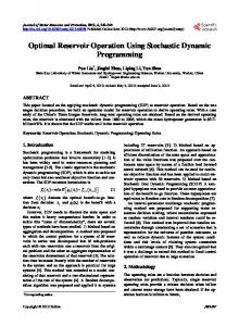
Figure 2: Maximum, minimum and median possible values for the expected daily cost using an infinite planning horizon, for both the arc-traversed (solid lines) and the chord-traversed (dashed lines) distance metrics. Dots mark the location of minima. in agreement with the value given in [5] (setting the cost discount over time to zero). However, more generally, solving qθ2 + 2qπθ − 2π dQ(q) = =0 (14) dθ (π + θ)2 gives us the threshold which minimizes the 100q th quantile, r 2π − π, (15) θ = π2 + q for which Equation (13) is the case where q=1. The median, for which q=0.5, is minimized at p θ = π 2 + 4π − π. (16) Obtaining the complete distribution function has the advantage that we can optimize any quantile that we like. In some cases we might, for instance, wish to select a threshold which minimizes the the 5th or 95th quantile. This is particularly interesting in the case where the maximum possible cost is threshold-invariant but lower quantiles are not; such an example, obtained using an alternative geometry to those presented in this paper, is shown in Figure 3.
The Euclidean distance metric, however, turns out to be more intractable. We have been unable to find an analytical value for θ which minimizes the maximum possible value of CSS for the chord-traverse metric, but Maple provides a numerical value of approximately 0.908129. The
WCECS 2010
Proceedings of the World Congress on Engineering and Computer Science 2010 Vol II WCECS 2010, October 20-22, 2010, San Francisco, USA
[3] RB Ash. Information Theory. Courier Dover Publications, New York, 1990.
1.4 1.2
[4] G Casella and RL Berger. Statistical Inference. Duxbury, Pacific Grove, second edition, 2002.
Cost
1
0.4
[5] AJ Kleywegt, MWP Savelsbergh and E Uyar. “A Stochastic Dynamic Routing Problem”, submitted, 2009. Available at http://www2.isye.gatech.edu/ ∼mwps/publications/.
0.2
[6] TA Severini. Elements of Distribution Theory. Cambridge University Press, New York, 2005.
0.8 0.6
0
0.2
0.4
0.6 0.8 Threshold
1
1.2
1.4
Figure 3: Contour plot of exected daily cost for an alternate geometry, along with maximum and minimum costs observed in 106 simulations (thick lines). √ The theoretical maximum (the 100th percentile) is 2, but here the 99.9999th quantile almost dips as low as 1.05. quantile function also appears to be intractable at this stage. In all cases, however, simulations can be used to estimate the optimal threshold for any aspect of the problem, and were employed at each stage of this work as an invaluable sanity check for our derivations.
6
Conclusions and Future Work
We have investigated an interesting problem from the operations research field from the point of view of mathematical statistics, allowing us to derive analytical expressions for the distribution of some interesting geometric transformations of random variates, as well as of cost functions in the stochastic dynamic scheduling problem. By using this approach we are able to generalize the optimal threshold for arbitrary quantiles of the cost function’s distribution. Many avenues of future directions are available, including extension to a two-dimensional subset of the Euclidean plane, which we are currently examining. Another area of particular interest is stochastic capacity, such as capacity fluctuations due to equipment failure.
References [1] E Angelelli, MG Speranza and MWP Savelsbergh. “Competitive Analysis for Dynamic Multiperiod Uncapacitated Routing Problems”, Networks 49:308– 317, 2009. [2] E Angelelli, MWP Savelsbergh and MG Speranza. “Competitive Analysis of a Dispatch Policy for a Dynamic Multi-period Routing Problem”, Operations Research Letters 35:713–721, 2007.
ISBN: 978-988-18210-0-3 ISSN: 2078-0958 (Print); ISSN: 2078-0966 (Online)
WCECS 2010