Optimizing and Tuning the Fast Multipole Method for State-of-the-Art ...

Optimizing and Tuning the Fast Multipole Method for State-of-the-Art Multicore Architectures Aparna Chandramowlishwaran?† , Samuel Williams? , Leonid Oliker? , Ilya Lashuk† , George Biros† , Richard Vuduc† ? †

CRD, Lawrence Berkeley National Laboratory, Berkeley, CA 94720 College of Computing, Georgia Institute of Technology, Atlanta, GA

Abstract

Approach: Specifically, we consider implementations of the kernel-independent FMM (KIFMM) algorithm [16], which simplifies the integration of FMM methods in practical applications (Section 2). The KIFMM itself is a complex computation, consisting of six distinct phases, all of which we parallelize and tune for leading multicore platforms (Section 4). We develop both single- and double-precision implementations, and consider numerous performance enhancements, including: low-level instruction selection, SIMD vectorization and scheduling, numerical approximation, data structure transformations, OpenMP-based parallelization, and tuning of algorithmic parameters. Our implementations are analyzed on a diverse collection of dual-socket multicore systems, including those based on the Intel Nehalem, AMD Barcelona, Sun Victoria Falls, and NVIDIA GPU processors. (Section 5). Key findings and contributions: Our main contribution is the first in-depth study of multicore optimizations and tuning for KIFMM, which includes crossplatform evaluations of performance, scalability, and power. We show that optimization and OpenMP parallelization can improve double-precision performance by 25× on Intel’s Nehalem, 9.4× on AMD’s Barcelona, and 37.6× on Sun’s Victoria Falls. Moreover, we compare our single-precision results against the literature’s best GPU-accelerated implementation [9]. Surprisingly, we find that the most advanced multicore architecture (Nehalem) reaches parity in performance and power efficiency with NVIDIA’s most advanced GPU architecture. Our results lay solid foundations for future ultra-scalable KIFMM implementations on current and emerging high-end systems.

This work presents the first extensive study of singlenode performance optimization, tuning, and analysis of the fast multipole method (FMM) on modern multicore systems. We consider single- and double-precision with numerous performance enhancements, including low-level tuning, numerical approximation, data structure transformations, OpenMP parallelization, and algorithmic tuning. Among our numerous findings, we show that optimization and parallelization can improve doubleprecision performance by 25× on Intel’s quad-core Nehalem, 9.4× on AMD’s quad-core Barcelona, and 37.6× on Sun’s Victoria Falls (dual-sockets on all systems). We also compare our single-precision version against our prior state-of-the-art GPU-based code and show, surprisingly, that the most advanced multicore architecture (Nehalem) reaches parity in both performance and power efficiency with NVIDIA’s most advanced GPU architecture.

1

Introduction

This paper presents the first extensive study of single-node performance optimization, tuning, and analysis of the fast multipole method (FMM) [5] on state-of-the-art multicore processor systems. We target the FMM because it is broadly applicable to a variety of scientific particle simulations used to study electromagnetic, fluid, and gravitational phenomena, among others. Importantly, the FMM has asymptotically optimal time complexity with guaranteed approximation accuracy. As such, it is among the most attractive solutions for scalable particle simulation on future extreme scale systems. This study focuses on single-node performance since it is a critical building-block in scalable multi-node distributed memory codes and, moreover, is less well-understood.

978-1-4244-6443-2/10/$26.00 ©2010 IEEE

2

Fast Multipole Method

This section provides an overview of the fast multipole method (FMM), summarizing the key components that are relevant to this study. For more in-depth algorithmic details, see Greengard, et al. [5, 16]. 1

V

V

V

V

U

U

V

V

B  

U

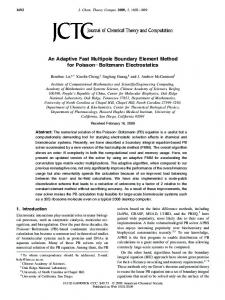
in 3-D or quadrant in 2-D) becomes a tree node whose children are its immediate sub-boxes. During construction, we associate with each node one or more neighbor lists. Each list has bounded constant length and contains (logical) pointers to a subset of other tree nodes. These are canonically known as the U , V , W , and X lists. For example, every leaf box B ∈ leaves(T ) has a U list, U (B), which is the list of all leaves adjacent to B. Figure 1 shows a quad-tree example, where neighborhood list nodes for B are are labeled accordingly. Tree construction has O(N log N ) complexity, and so the O(N ) optimality refers to the evaluation phase (below). However, tree construction is typically a small fraction of the total time; moreover, many applications build the tree periodically, thereby enabling amortization of this cost over several evaluations. Evaluation: Given the tree T , evaluating the sums consists of six distinct computational phases: there is one phase for each of the U , V , W , and X lists, as well as upward (up) and downward (down) phases. These phases involve traversals of T or subsets of T . Rather than describe each phase in detail, which are welldescribed elsewhere [5, 15, 16], we summarize the main algorithmic characteristics of each phase in Table 1. For instance, in the U list phase, we traverse all leaf nodes, where for each leaf node B ∈ leaves(T ) we perform a direct evaluation between B and each of the nodes B 0 ∈ U (B). For each leaf B, this direct evaluation operates on O(q) points and has a flop cost of O(q 2 ) for each box. By contrast, the V-list operates on O(q) points and performs O(q log q) flops for each box, and so has lower computational intensity. Generally, we expect the cost of the U-list evaluation phase to dominate other phases when q is sufficiently large. There are multiple levels of concurrency during evaluation: across phases (e.g., the upward and U-list phases can be executed independently), within a phase (e.g., each leaf box can be evaluated independently during the U-list phase), and within the per-octant computation (e.g., vectorizing each direct evaluation). In this paper, we consider intra-phase and per-octant parallelization only, essentially using OpenMP and manual SIMD parallelization, respectively. For the Upward and Downward phases, which both involve tree traversals, there is a obvious dependency between a parent and its child boxes. However, the children themselves are independent and can be computed concurrently with the amount of work per level increasing toward the leaves. Related work: For parallel FMM, most of the recent work of which we are aware focuses on distributed memory codes with GPU-based acceleration [1,6,9,12]. Indeed, the present study builds on our own state-of-theart parallel 3-D KIFMM implementation, which uses MPI+CUDA [9]. However, these works have not yet considered conventional multicore acceleration and tun-

U

V

U U

U U U W W W W W

W

V

U

V

V

V

V

V

V

V

V

W

W

W

X

W

X

Figure 1. U, V, W, and X lists of a tree node B for an adaptive quadtree in 2-D.

Given a system of N source particles, with positions given by {y1 , . . . , yN }, and N targets with positions {x1 , . . . , xN }, we wish to compute the N sums, f (xi ) =

N X

K(xi , yi ) · s(yj ),

i = 1, . . . , N

(1)

j=1

where f (x) is the desired potential at target point x; s(y) is the density at source point y; and K(x, y) is an interaction kernel that specifies “the physics” of the problem. For instance, the single-layer Laplace ker1 1 nel, K(x, y) = 4π ||x−y|| , might model electrostatic or gravitational interactions. Evaluating these sums appears to require O(N 2 ) operations. The FMM instead computes approximations of all of these sums in optimal O(N ) time with a guaranteed user-specified accuracy, where the desired accuracy changes the complexity constant [5]. The FMM is based on two key ideas: (i) a tree representation for organizing the points spatially; and (ii) fast approximate evaluation, in which we compute summaries at each node using a constant number of tree traversals with constant work per node. We implement the kernel independent variant of the FMM, or KIFMM [16]. KIFMM has the same structure as the classical FMM [5]. Its main advantage is that it avoids the mathematically challenging analytic expansion of the kernel, instead requiring only the ability to evaluate the kernel. This feature of the KIFMM allows one to leverage our optimizations and techniques and apply them to new kernels and problems. Tree construction: Given the input points and a user-defined parameter q, we construct an oct-tree T (or quad-tree in 2-D) by starting with a single box representing all the points and recursively subdividing each box if it contains more than q points. Each box (octant 2

Phase Upward U-list V-list X-list W-list Downward

Computational Complexity O(N p + M p2 ) O(27N q) O(M p3/2 logp + 189M p3/2 ) 0 uniform distribution O(N q) non-uniform distribution 0 uniform distribution O(N q) non-uniform distribution O(N p + M p2 )

Algorithmic Characteristics postorder tree traversal, small† matvecs direct computation as in Equation 1 (matvecs on the order of q) consists of small FFTs, pointwise vector multiplication (convolution) matvecs matvecs preorder tree traversal, small† matvecs

Table 1. Characteristics of the computational phases in KIFMM. N is the number of source particles, the number of boxes is M ∼ N/q and p denotes the number of expansion coefficients. The user chooses p to trade-off time and accuracy, and may tune q to minimize time. † Size is determined by the chosen accuracy, generally smaller than q.

3.1

ing. In Section 5, we compare our multicore optimizations to this prior use of GPU acceleration, with the perhaps surprising finding that a well-tuned multicore implementation can match a GPU code. Coulaud, et al., propose Pthreads- and multithreaded BLAS-based multicore parallelization within node [3]. However, we use a larger set of optimizations and provide cross-platform performance and power analysis.

This section summarizes the key differences, as they pertain to the FMM, among the three dual-socket multicore SMPs used in this study: Intel’s quad-core Xeon (Nehalem), AMD’s quad-core Opteron (Barcelona), and Sun’s chip-multithreaded, eight-core UltraSparc T2+ (Victoria Falls). Our final analysis references our prior GPU-only accelerated results [9]. The key parameters of these systems appear in Table 2. Basic microarchitectural approach: Nehalem and Barcelona are x86, superscalar, out-of-order architectures with large per-thread caches and hardware prefetchers. Victoria Falls, by contrast, employs finegrained chip multithreading (CMT) and smaller perthread caches. Consequently, Victoria Falls requires the programmer to express roughly an order of magnitude more parallelism than the x86 systems in order to achieve peak performance or peak bandwidth. Luckily, there is ample fine-grained thread-level parallelism in the FMM. Computational peak: The two x86-based systems have similar peak floating-point performance, but 4× higher than Victoria Falls partly due to the SIMD units on x86. SIMD enables up to to 4 flops (multiply and add) per cycle per core in double-precision (DP) and 8 in single-precision (SP). Because the FMM has high computational intensity in at least one of its major phases (U-list), we may expect superior performance on the x86 systems compared to Victoria Falls. Unfortunately, many kernels K(x, y) also require square root and divide operations, which on all three systems are not pipelined and therefore are extremely slow. For example, on Nehalem, double-precision divide and square root run at 0.266 GFlop/s (5% of peak multiply/add performance) and 0.177 GFlop/s (3%), respectively. To address this deficiency, both x86 systems (but not Victoria Falls) have a low latency and pipelined single-precision approximate reciprocal square-root op-

There are numerous non-GPU studies of single-core distributed memory FMM implementations [8, 11] (see also references in Ying, et al. [15]), most based on the classical tree-based N-body framework of Warren and Salmon [14], including our own prior KIFMM work [9, 15]. Researchers have considered a variety of data structures with attractive communication properties, again in the distributed context [7]. To our knowledge, the present study is the first to consider extensive multicore-centric optimizations, data structures, and cross-platform analysis. For direct O(N 2 ) methods, tuning, and specialpurpose hardware (e.g. MDGRAPE), see the references in related papers [2, 10].

3

Architectures

Experimental Setup

We explore FMM performance as we vary architecture, floating-point precision, and initial particle distribution. To facilitate comparisons to prior work, we select a commonly used kernel K (Laplace kernel in Section 2). The desired accuracy is fixed to a typical minimum setting that is also sensible for single-precision (yielding 4–7 decimal digits of accuracy). Moreover, because tuning can dramatically change the requisite number of floating-point operations, we define and defend our alternate performance metrics. These aspects are discussed in detail below. 3

Architecture Frequency (GHz) Sockets Cores/Socket Threads/Core SIMD (DP, SP) GFlop/s (DP, SP) rsqrt/s∗ (DP, SP) L1/L2/L3 cache local store DRAM Bandwidth Power Compiler

Intel X5550 (Nehalem) 2.66 GHz 2 4 2 2-way 4-way 85.33 170.6 0.853 42.66 32/256/8192† KB — 51.2 GB/s 375W icc 10.1

AMD 2356 (Barcelona) 2.30 GHz 2 4 1 2-way 4-way 73.60 146.2 0.897 73.60 64/512/2048† KB — 21.33 GB/s 350W icc 10.1

Sun T5140 (Victoria Falls) 1.166 GHz 2 8 8 1 1 18.66 18.66 2.26 — 8/4096† KB — 64.0 GB/s 610W cc 5.9

NVIDIA T10P (S1070) 1.44 GHz 2 (+2 CPUs) 30 (GPU) 8 (GPU) 1 8-way N/A 2073.6 N/A 172.8 — 16 KB 204 GB/s 325W+400W‡ nvcc 2.2

Table 2. Architectural Parameters. All power numbers, save the GPU, we obtained using a digital power meter. ∗ reciprocal square-root approximate. † shared among cores on a socket. ‡ max server power (of which the 2 active CPUs consume 160W) plus max power for two GPUs.

eration ( √1x ) that we can exploit to accelerate doubleprecision computations [10]. Memory systems: Nehalem has a much larger L3 cache and much higher peak DRAM bandwidth. This should enable better performance on kernels with large working sets. However, Nehalem also has smaller L1 and L2 caches, yielding a per-thread cache footprint that is 41 that of Barcelona, suggesting performance will be similar for computations with small working sets and high computational intensity. The FMM phases exhibit a mix of input-dependent behaviors, and so the ultimate effects are not entirely clear a priori. Comparisons to GPU: Our prior work applied GPU acceleration to KIFMM on the NCSA Lincoln Cluster [9], where each node is a dual-socket × quad-core Xeon 5410 (Harpertown) CPU server paired with two NVIDIA T10P GPUs. We use the CPUs only for control, and run all phases (except tree construction) on the GPUs. That is, there is one MPI process on each socket, and each process is assigned to one GPU; processes communicate via message passing and to their respective GPUs via PCIe. For our energy comparisons, we bound power using two configurations: aggregate peak GPU power plus zero CPU power, and aggregate peak GPU power plus the peak CPU power. With 12× the compute capacity and over 5× the bandwidth, one would na¨ıvely expect the GPU implementation to considerably outperform all other platforms. 3.2

recognized importance [16]. Precision: We consider both single and doubleprecision in our study. Single-precision is an interesting case for a variety of reasons. First, an application may have sufficiently low accuracy requirements, due to uncertainty in the input data or slow time-varying behavior. In this case, using single-precision can yield significant storage and performance benefits. Next, on current x86 architectures, SIMD instructions are 2-wide in double precision and 4-wide in single. However, forthcoming x86 Advanced Vector Extensions (AVX) will double these widths. As such, using single precision SIMD on today’s Nehalem is a proxy for double precision performance on tomorrow’s Sandy Bridge. Finally, current architectures provide fast reciprocal square-root methods in single-precision, but not double. By exploring the benefits in single, we may draw conclusions as to potential benefit future architectures may realize by implementing equivalent support in double. Accuracy: One of the inputs to FMM is numerical accuracy desired in the final outcome, expressed as the desired “size” of the multipole expansion. In our experiments, we choose the desired accuracy to deliver the equivalent of 6 decimal digits in double-precision and 4 digits in single. We verify the delivered accuracy of our all of our na¨ıve, optimized, parallel, and tuned implementations. 3.3

Kernel, Precision, and Accuracy

Particle Distributions

We examine two different particle distributions namely, a spatially uniform and a spatially non-uniform (elliptical or ellipsoidal) distribution. The uniform case is analyzed extensively in prior work; the non-uniform case is where we expect tree-based methods to deliver performance and accuracy advantages over other nu-

In this section, we describe the interaction kernel, precision, and desired accuracy, and their implications for implementation and optimization. Kernel: Following prior work, we use the singlelayer Laplacian kernel (Section 2) owing to its widely4

Tree

Up

U-list

V-list

W-list

X-list

Down

SIMDization Newton-Raphson SOA∗ layout Matrix-free FFTW

efficiency (evaluations per Joule).

— N/A x86 N/A N/A

x86 x861 x86 X N/A

x86 x861 x86 X N/A

— N/A x86 X X

x86 x861 x86 X N/A

x86 x861 x86 X N/A

x86 x861 x86 X N/A

X X

X X

X X

X X

X X

X X

We applied numerous optimizations to the various computational phases (Section 2). Beyond optimizations traditionally subsumed by compilers, we apply numerical approximations, data structure changes, and tuning of algorithmic parameters. Table 3 summarizes our optimizations and their applicability to the FMM phases and our architectures. Note that not all optimizations apply to all phases. Figure 2 presents the cumulative benefit as each optimization is successively applied to the serial reference KIFMM implementation [16]. We will refer to this figure repeatedly as we describe each optimization. If an optimization has associated tuning parameters (e.g.unrolling depth), we tune it empirically.

OpenMP — Tuning for best q X

4

Table 3. FMM optimizations attempted in our study for Nehalem and Barcelona (x86) or Victoria Falls (VF). ∗ Structures of arrays (SOA) layout. 1 double-precision only. A “X” denotes all architectures, all precisions.

4.1

SIMDization

We found it necessary to apply SIMD vectorization manually, as the compiler was unable to do so. All Laplacian kernel evaluations and point-wise matrix multiplication (in the V-list) are implemented using SSE intrinsics; specifically, in double-precision, we use SSE instructions like addpd, mulpd, subpd, divpd, and sqrtpd. Note that the Laplacian kernel performs 10 flops (counting each operation as 1 flop) per pairwise interaction, and includes both a square-root and divide. In single-precision on x86, there is a fast (pipelined) approximate reciprocal square-root instruction: rsqrtps. As such, with sufficient instructionand data-level parallelism, we may replace the traditional scalar fsqrt/fdiv combination with not simply a sqrtps/divps combination, but entirely with one rsqrtps. Doing so enables four reciprocal square-root operations per cycle without compromising our particular accuracy setting. Figure 2 shows the speedup from SIMDization. The top three figures in Figure 2 use an uniform particle distribution and the bottom three use an elliptical distribution. SIMD nearly doubles Nehalem performance for all kernels except V-list, where FFTW (see Section 4.5) is already SIMDized. The benefit on Barcelona was much smaller (typically less than 50%), which we will investigate in future work. As there are no double precision SIMD instructions in SPARC/Victoria Falls, SIMD related optimizations are not applicable.

merical paradigms (e.g., particle-mesh methods). In both cases, our test problems use 4 million source particles plus an additional 4 million target particles. Uniform: In this case, we distribute points uniformly at random within the unit cube. In 3D, for boxes not on the boundary, the U-list (neighbor list) contains 27 boxes and the V-list (interaction list) contains 189 boxes. The X- and W-lists are empty since the neighbors of a box are adjacent boxes in the same level. Thus, the time spent in the various list computations will differ from the non-uniform case and tuning will favor a different value for q, the maximum points per box. Elliptical: In this case, particles are angularlyuniformly (in spherical coordinates) distributed on the surface of an ellipsoid with an aspect ratio 1:1:4. For an uniform distribution, a regular octree is constructed. However, the elliptical case requires an adaptively refined octree. As such, the depth of the computation tree could be quite large, resulting in high tree construction times as shown in Figure 5. 3.4

Optimizations

Performance Metrics

Since our optimizations and tuning of q can dramatically change the total number of floating-point operations, we use time-to-solution (in seconds) as our primary performance metric rather than GFlop/s In our final comparison, we present relative performance (evaluations per second), where higher numbers are better. This choice has ramifications when assessing scalability. In particular, rather than examining GFlop/s/core or GFlop/s/thread to assess per-core (or per-thread) performance, we report thread-seconds: that is, the product of execution time by the number of threads. When it comes to energy efficiency, we present the ratio relative to the optimized and parallelized Nehalem energy

4.2

Fast Reciprocal Square Root

A conventional double-precision SIMDized code would perform the reciprocal square-root operation using the intrinsics sqrtpd and divpd as above. Unfortunately, these instructions have long latencies (greater than 20 cycles) and cannot be pipelined, thus limiting performance. As we have abundant 5

300%

50%

150%

Down

X list

W list

Tree

X list

V list

W list

U list

Down

35% 30% 25% 20% 15% 10%

+Newton-Raphson Approximation

X list

Down

W list

V list

U list

5% Up

-50% Down

-100%

X list

0%

V list

0%

W list

50%

Up

Up

100%

100%

U list

40%

Tree

200%

45%

+Structure of Arrays

0%

+Matrix-Free Computation

Down

300%

Victoria Falls

50%

X list

200%

55%

Barcelona

W list

400%

Tree

0%

speedup

250%

speedup

500%

+SIMDization

5%

300%

Nehalem

20% 10%

Tree

Down

X list

V list

W list

Up

U list

Tree 600%

-50%

25% 15%

0%

-100%

30%

V list

0%

speedup

100%

35%

V list

100%

150%

Up

200%

40%

U list

300%

45%

Up

200%

U list

400%

Victoria Falls

50%

Tree

250%

55%

Barcelona

speedup

Nehalem

500%

speedup

speedup

600%

+FFTW

Figure 2. Speedup over the double-precision reference code. Top: Uniform distribution. Bottom: Elliptical distribution. Note, W- and X- lists are empty for the uniform case. SIMD, Newton-Raphson, and data structure transformations were not implemented on Victoria Falls.

instruction-level parallelism, we can exploit x86’s fast single-precision reciprocal square-root instruction to accelerate the double-precision computations [10]. That is, we replace the sqrtpd/divpd combination with the triplet, cvtpd2ps (convert double to single)/rsqrtps/cvtps2pd (single to double). To attain the desired accuracy, we apply an additional NewtonRaphson refinement iteration. This approach requires more floating-point instructions, but they are low latency and can be pipelined. Figure 2 shows that the Newton-Rapshon approach improves Nehalem performance by roughly 100% over SIMD. Since there are relatively few kernel evaluations in the V-list, we don’t see an appreciable benefit. Surprisingly, the benefit on Barcelona is relatively modest; the cause is still under investigation. 4.3

ery point and unrolling the inner loop twice (or 4 times in single-precision). Instead, we explore using the structure-of-arrays (SOA) or structure splitting layout [17] in which the components are stored in separate arrays. This transformation simplifies SIMDization since we can load two (or four) components into separate SIMD registers using a single instruction. Changing the data layout further improved the overall U-list performance on Nehalem up to 300% speedup over the reference. The transformation does not affect the V-list phase due to its relatively low computational intensity. Moreover, the data layout change substantially improved Barcelona performance on most phases.

Structure-of-Arrays Layout

Unfortunately, the data layout change increased tree construction time due to lack of spatial locality. This tradeoff (dramatically reduced computational phase time for slightly increased tree construction time) is worthwhile if tree construction time is small compared to the total evaluation execution time.

Our reference implementation uses an array-ofstructures (AOS) data structure where all components of a point are stored contiguously in memory (e.g. x1 , y1 , z1 , x2 , y2 , z2 , ..., xn , yn , zn ). This layout is not SIMD-friendly as it requires a reduction across ev6

4.4

Matrix-free calculations

execution time. Second, in many real simulation contexts, particle dynamics may be sufficiently slow that tree reconstruction can be amortized. Future work will involve parallelization of tree construction keeping in mind both uniform and non-uniform distributions.

To use tuned vendor BLAS routines, our reference code explicitly constructs matrices to perform matrixvector multiplies (matvecs), as done by others [3]. However, we can apply what is essentially interprocedural loop fusion to eliminate this matrix, instead constructing its entries on-the-fly and thereby reducing the cache working set and memory traffic. For example, recall that the U-list performs a direct evaluation like Equation 1, which is a matvec, between two leaf boxes. Rather than explicitly constructing the kernel matrix K and performing the matvec, we can fuse the two steps and never store this matrix, reducing the memory traffic from O(q 2 ) to O(q), if the maximum points per box is q. The idea applies to the Up(leaf), Wlist, X-list, and Down(leaf) phases as well; the matrices arise in a different way, but the principle is the same. As seen in Figure 2, this technique improves Nehalem performance by an additional 25%, and often improved Barcelona and Victoria Falls performance by better than 40%. Cumulatively including this optimization (aside from V-list) improved Nehalem performance by more than 400%, Barcelona by more than 150%, and Victoria Falls by 40%. 4.5

4.7

After applying serial optimization, we parallelize all phases via OpenMP. We apply inter-box parallelization for all phases except Upward and Downward. That is, we assign a chunk of leaf boxes to each thread and exploit parallelism within each phase. For Upward and Downward which has dependencies across the levels of the tree, we exploit the concurrency at each level. By convention, we exploit multiple sockets, then multiple cores, and finally threads within a core. Algorithmically, the FMM is parameterized by the maximum number of particles per box, q. As q grows, the U-list phase quickly increases in cost even as other phases become cheaper as the tree height shrinks; this dependence is non-trivial to predict, particularly for highly non-uniform distributions. We exhaustively tune q for each implementation on each architecture, as discussed in Section 5. Auto-tuning q will be the subject of our future work.

FFTW

5

In our KIFMM implementation, the V-list phase consists of (i) small forward and inverse FFTs, once per source/target box combination; and (ii) pointwise multiplication I times for each target box, where I is the number of source boxes in said target box’s V-list. Local FFTs are performed using FFTW [4]. Typically, one executes an FFTW plan for the array with which the plan was created using the function fftw execute. As the sizes and strides of the FFTs in V-list are not only quite small but are also identical, we may create a single plan and reuse it for multiple FFTs, using the fftw execute dft r2c function. We ensure alignment by creating the plan with the FFTW UNALIGNED flag coupled with an aligned malloc(). FFTW only benefits V-list computations. Nevertheless, on both x86 machines, FFTW substantially improved V-list performance for elliptical distributions. The benefit on uniform distributions was less dramatic since the relative time spent in the V-list tends to be smaller. Unfortunately, Victoria Falls saw little benefit from the plan reuse within FFTW; this will be addressed in future work. 4.6

Parallelization and Tuning

Performance Analysis

The benefits of optimization, threading, and tuning are substantial. When combined, these methods delivered speedups of 25×, 9.4×, and 37.6× for Nehalem, Barcelona, and Victoria Falls, respectively, in doubleprecision for the uniform distribution; and 16×, 8×, and 24×, respectively, for the elliptical case. In this section we first tune our parallel implementation for the FMM’s key algorithmic parameter, q, the maximum particles per box. We then analyze the scalability for each architecture. Finally, we compare the performance and energy efficiency among architectures. 5.1

Tuning particles per box

Figure 3(a) presents the FMM execution time as a function of optimization, parallelization, and particles per box q on Nehalem with an elliptical particle distribution. Although we performed this tuning for all architectures, particle distributions, and precisions, we only present Nehalem data due to space limitations. The optimal setting of q varies with the level of optimization, with higher levels of optimization enabling larger values of q. Since we did not parallelize tree construction, we consider just the evaluation time in Figure 3(b). Thus, one should only tune q (or other parameters affected by parallelization) after all other optimizations have been applied and tuned. Figure 3(c) decomposes evaluation time by phase. The Upward traversal, Downward traversal, and V-list

Tree Construction

There are numerous studies of parallel tree construction [1,7,13]. In this paper, we focus on accelerating the evaluation phases of FMM for two main reasons. First, tree construction initially constituted a small fraction of 7

600

Tree Construction+Evaluation Reference Serial Optimized Serial Optimized Parallel

500

400 Seconds

Seconds

300

300

184 20.1 50

100

250

500

750

Maximum Particles per Box

6.0

2.0 10.4

0

0

8.0

4.0

168 100

100

Up U list V list W list X list Down

10.0

200

200

Breakdown by List

12.0

Reference Serial Optimized Serial Optimized Parallel

500

400

14.0

Force Evaluation Only

Seconds

600

50

100

250

500

0.0 750

Maximum Particles per Box

50

100

250

500

750

Maximum Particles per Box

(a) (b) (c) Figure 3. Tuning q, the maximum number of particles per box. Only Nehalem, elliptical distribution data is shown. There is contention between decreasing Up, Down, and V-list time, and increasing U-list time. Note, tree construction time scales like Up, Down, and V-list times.

execution times decrease quickly with increasing q. However, execution time for the other lists, especially U-list, grow with increasing q. Observe a crossover point of q = 250 where time saved in Up, Down, and Vlist can no longer keep pace with the quickly increasing time spent in U-list. 5.2

dominates the overall evaluation time and delivers very good scalability to 8 cores. This observation is not surprising since this phase has high arithmetic intensity. However, the V-list computations, which initially constitute a small fraction of overall time, show relatively poorer scalability, eventually becoming the bottleneck on Nehalem. The V-list has the lowest arithmetic intensity and is likely suffering from bandwidth contention. The other two kernels show good scalability to 4 cores, but remain a small fraction of the overall time. Barcelona shows good scalability to four cores (2 per socket) but little thereafter. The bottom figure shows the problem: U-list scalability varies some but is reasonably good, while the V-list scales poorly and eventually constitutes 50% more time than U-list. Given Barcelona’s smaller L3 cache and diminished bandwidth, the effects seen on Nehalem are only magnified. Victoria Falls, with its ample memory bandwidth and paltry floating-point capability, scales perfectly to 16 cores (lines are almost perfectly flat). Once again, performance is dominated by the U-list. As multithreading within a core is scaled, the time required for U-list skyrockets. Although, we manage better than a 2× speedup using four threads per core, we see none thereafter. Figure 5 extends these results to the non-uniform elliptical distribution, which will now include W- and X-list phases. On x86, for the same number of particles, the elliptical time-to-solution is less than the uniform case. This occurs because more interactions can be pruned in the non-uniform case. However, as a consequence, tree construction also becomes a more severe impediment to scalability. As with the uniform distribution, evaluation time scales well on Nehalem up to 8 threads (one thread per core). Thereafter, it reaches parity with tree construction time. Additional cores or optimization yield only

Scalability

Exploiting multicore can be challenging as multiple threads share many resources on a chip like caches, bandwidth, and even floating-point units. Thus, the benefit of thread-level parallelism may be limited. Figure 4 presents the performance scalability by architecture as a function of thread-level parallelism for the double-precision, uniform distribution case (thus, has no W or X list phases). Threads are assigned first to multiple sockets before multiple cores, and multiple cores before simultaneous multithreading (SMT). For clarity, we highlight the SMT region explicitly. On all machines, the 2 thread case represents one thread per socket. The top figures show overall times for two cases: (i) assuming tree construction before evaluation, and (ii) the asymptotic limit in which the tree is constructed once and can be infinitely reused. (Recall that tree construction was the only kernel not parallelized.) Observe that Nehalem delivers very good scalability to 8 threads at which point HyperThreading provides no further benefit. Unfortunately, the time required for tree construction becomes a substantial fraction of the overall time. Thus, further increases in core count will deliver sublinear scaling due to Amdahl’s Law. In the bottom figures, we report thread-seconds to better visualize the scalability of the code for each phase. A flat line denotes perfect scalability and a positive slope denotes sublinear scaling. The U-list initially 8

New tree constructed for every force evaluation 200

75

100

8

Threads 200

Nehalem

90

4

Threads

Barcelona

175

70 60 50 40 30 20

150

Thread-Seconds

Thread-Seconds

80

125 100 75 50 25

10

0 1

2

4

8

16

1

Threads

2

4

8

Threads

Upward

U-list

Victoria Falls

1

0

6500 6000 5500 5000 4500 4000 3500 3000 2500 2000 1500 1000 500 0

Threads

V-list

128

Threads

2

64

0 1

16

128

8

32

4

64

2

4

1

300 16

0

32

0

600

16

25

1

10

1200 900

50

20

1500

8

30

1800

8

40

100

4

50

2100

125

Seconds

Seconds

Seconds

2400

150

60

Victoria Falls

2700

175

70

Thread-Seconds

3000

Barcelona

2

Nehalem

80

2

90

asymptotic limit (force evaluation time only)

Downward

Figure 4. Double-precision, multicore scalability using OpenMP for a uniform particle distribution. Top: time as a function of thread concurrency showing relative time between list evaluations and tree construction. Bottom: break down of evaluation time by list. Note: “Threadseconds” is essentially the inverse of GFlop/s/core, so flat lines denote perfect scaling:

an additional 2× speedup. Also observe that the relative time of each phase changes. U-list time dominates at all concurrencies, and V-list time scales well since the V-lists happen to have fewer boxes for this distribution. The behavior on Barcelona is similar except, the Ulist time scales somewhat more poorly with the elliptical distribution than in the uniform case. Interestingly, most phases scale poorly in the multicore region on Victoria Falls, though U-list time still dominates. 5.3

is more than 3× faster. Although the initial performance differences are expected given the differences in frequency, the final difference is surprising as Nehalem has comparable peak performance and only about twice the bandwidth. Moreover, and unexpectedly, with only 4.5× the peak flops Nehalem is as much as 10× faster than Victoria Falls. Victoria Falls’ small per-thread cache capacity may result in a large number of cache misses. Across the board, we observe the benefit of tree construction amortization is nearly a factor of two.

Architectural Comparison

Unlike the scalar Victoria Falls, x86 processors can more efficiently execute single-precision operations using 4-wide SIMD instructions. GPUs take this approach to the extreme with an 8-wide SIMD-like implementation. To that end, we repeated all optimizations, parallelization, and tuning for all architectures and distributions in single-precision. We then re-ran the GPUaccelerated code of prior work by Lashuk, et al. [9].

Beyond the substantial differences among architectures in serial speedups, tuning, and multicore scalability, we observe that the raw performance among processors differs considerably as well. Moreover, performance varies dramatically with floating-point precision. Figure 6 compares the double-precision performance for our three machines for both particle distributions. For each distribution, performance is normalized to the reference Nehalem implementation. Initially, Nehalem is only about 25% faster than Barcelona; however, after optimization, parallelization, and tuning, Nehalem

For the GPU comparison, we consider 1 node (2 CPU sockets) with either 1 GPU or 2 GPUs. The GPUs perform all phases except tree construction, with 9

New tree constructed for every force evaluation 180

2400 2100

120

1200

60

900 600

30

300

1

200

8

Threads 6000

Barcelona

60 50 40 30 20

125 100 75 50

10

25

0

0 1

2

4

8

16

4500 4000 3500 3000 2500 2000 1500 1000 500 0

1

Threads

Upward

5000

150

2

4

8

1

70

Thread-Seconds

Thread-Seconds

80

Victoria Falls

5500

175

Threads

U-list

Threads

V-list

W-list

X-list

128

Nehalem

90

2 4 Threads

64

16

128

8

32

4 Threads

64

100

2

32

1

16

0

0

1

0

16

10

8

20

8

30

1500

4

40

1800

90

4

50

Seconds

Seconds

Seconds

60

Victoria Falls

2700

150

70

Thread-Seconds

3000

Barcelona

2

Nehalem

80

2

90

asymptotic limit (force evaluation time only)

Downward

Figure 5. Double-precision, multicore scalability using OpenMP for an elliptical particle distribution. Top: Time as a function of thread concurrency, comparing evaluations and tree construction components. Bottom: Breakdown of evaluation time by list. Note: “Threadseconds” is essentially the inverse of GFlop/s/core, so flat lines indicate perfect scaling.

the CPU used only for control and thus largely idle. This experiment allows us to compare not only different flavors of homogenous multicore processors, but also compare them to heterogeneous computers specialized for single-precision arithmetic. Note that the GPU times include host-to-device data structure transfer times.

tage over Barcelona dropped to as little as 1.6× — which is still high given the architectural similarities. Perhaps the most surprising result is that with optimization, parallelization, and tuning, Nehalem is up to 1.7× faster than one GPU and achieves as much as 3 4 × the 2-GPU performance. Where Nehalem’s optimal particles per box was less than 250, GPUs typically required 1K to 4K particles per box. In order to attain a comparable time-to-solution, the GPU implementation had to be configured to prioritize the computations it performs exceptionally well — the computationally intense regular parallelism found in U-list.

These single-precision results appear in Figure 6. Barcelona saw the most dramatic performance gains of up to 7.2× compared with double-precision. This gain greatly exceeds the 2× increase in either the peak flop rate or operand bandwidth. Nehalem’s gains, around 4×, were also surprisingly high. Victoria Falls typically saw much less than a factor of two performance increase, perhaps due to nothing more than the reduction in memory traffic. We attribute this difference to x86’s single-precision SIMD advantage, as well as the ability to avoid the Newton-Raphson approximation in favor of one rsqrtps (reciprocal square root approximation) instruction without loss of precision.

5.4

Energy Comparison

We measured power usage using a digital power meter for our three multicore systems. As it was not possible to take measurements on the remote GPU-based system, we include two estimates: peak power (assuming full GPU and full CPU power) and maximum GPUonly power (assuming the CPUs consume zero power). We report the resultant power efficiency relative to parallelized and tuned Nehalem (higher is better). Figure 7

Although Nehalem’s performance advantage over Victoria Falls increased to as much as 21×, its advan10

+Tree Construction Amortized

1000

Uniform Distribution

Elliptical Distribution

4.25 2.14

2.84

61.0

4.63

3.02

5.61

1 0.1

Uniform Distribution

+2 GPUs

VF

+1 GPU

Nehalem

Barcelona

0.01 Nehalem

VF

Barcelona

Nehalem

VF

Barcelona

0.01

10

+2 GPUs

0.1

60.3

111

1

VF

104

100

+1 GPU

33.2

Energy assuming CPU consumes no power

Single Precision 3.32

11.4

45.9

10

Performance Relative to Out-of-the-box Nehalem

Double Precision 13.6

Nehalem

Performance Relative to Out-of-the-box Nehalem

100

+OpenMP

6.34

+Optimized

Barcelona

Reference

Elliptical Distribution

Figure 6. Performance relative to out-of-the-box Nehalem for each distribution. Note, performance is on a log scale. Labels show the final execution time (secs) after all optimizations.

lective understanding of the strengths and limits of using heterogeneous computers. Looking forward, we see numerous opportunities. First, we relied largely on bulk-synchronous parallelism, which resulted in working sets that did not fit in cache. Dataflow and work-queue approaches may mitigate this issue. Next, optimal algorithmic parameters like particles per box will vary not only with architecture, but also optimization and scale of parallelism. Finally, our manual SIMD transformations and their interaction with data layout was a significant performance win, and should be a priority for new compiler and/or programming model efforts.

shows this relative energy-efficiency as a function of architecture, distribution, and precision. Nehalem still manages a sizable energy efficiency over all other CPU architectures, although its energy advantage over Barcelona is less than its performance advantage. Conversely, the FBDIMM-based Victoria Falls consumes at least 66% more power than any other CPUbased machine. As such, for FMM, Nehalem is as much as 35× more energy-efficient than Victoria Falls. The GPU-based systems, by our estimates, consumes as much as 725W. Thus, Nehalem is as much as 2.37× and 1.76× more energy-efficient than systems accelerated using 1 or 2 GPUs, respectively. Even under the optimistic assumption that the largely idle CPUs consumed no power, then Nehalem’s energy-efficiency is still between 0.97× and 1.65×.

6

Acknowledgments We would like to thank the University of California Parallel Computing Laboratory for access to machines. All authors from LBNL were supported by the ASCR Office in the DOE Office of Science under contract number DE-AC02-05CH11231. Authors from UCB were also supported by Microsoft (Award #024263), Intel (Award #024894), and by matching funding by U.C. Discovery (Award #DIG07-10227). Authors at Georgia Tech were supported in part by the National Science Foundation (NSF) under award number 0833136, and grants from the Defense Advanced Research Projects Agency (DARPA) and Intel Corporation. Any opinions, findings and conclusions or recommendations expressed in this material are those of the authors and do not necessarily reflect those of NSF, DARPA, or Intel.

Conclusions

Given that single-node multicore performance and power efficiency will be critical to scalability on nextgeneration extreme scale systems, we believe our extensive study of parallelization, low-level and algorithmic tuning at run-time (i.e. the input-dependent maximum points per box, q), numerical approximation, and data structure transformations contributes a solid foundation for the execution of FMM on such machines. Surprisingly, given a roughly comparable implementation effort, a careful multicore implementation can deliver performance and energy efficiency on par with that of a GPU-based approach, at least for the FMM [9]. We believe this finding is a significant data point in our col11

Reference

+Optimized

+Tree Construction Amortized

10

Double Precision Power Efficiency Relative to Nehalem w/OpenMP

1

0.1

1

0.1

Uniform Distribution

Elliptical Distribution

Uniform Distribution

+1 GPU

+2 GPUs

VF

Barcelona

Nehalem

+2 GPUs

VF

+1 GPU

Nehalem

VF

Barcelona

Nehalem

VF

Barcelona

0.01 Nehalem

0.01

Energy assuming CPU consumes no power

Single Precision

Barcelona

Power Efficiency Relative to Nehalem w/OpenMP

10

+OpenMP

Elliptical Distribution

Figure 7. Energy efficiency relative to optimized, parallelized, and tuned Nehalem for each distribution. Note, efficiency is on a log scale. (higher is better).

References

[10] K. Nitadori, J. Makino, and P. Hut. Performance tuning of n-body codes on modern microprocessors: I. Direct integration with a Hermite scheme on x86 64 architecture. New Astron., 12:169–181, 2006. arXiv:astroph/0511062v1.

[1] P. Ajmera, R. Goradia, S. Chandran, and S. Aluru. Fast, parallel, GPU-based construction of space filling curves and octrees. In Proc. Symp. Interactive 3D Graphics (I3D), 2008. (poster).

[11] S. Ogata, T. J. Campbell, R. K. Kalia, A. Nakano, P. Vashishta, and S. Vemparala. Scalable and portable implementation of the fast multipole method on parallel comptuers. Computer Phys. Comm., 153(3):445–461, July 2003.

[2] N. Arora, A. Shringarpure, and R. Vuduc. Direct n-body kernels for multicore platforms. In Proc. Int’l. Conf. Par. Proc. (ICPP), Sep. 2009. [3] O. Coulaud, P. Fortin, and J. Roman. Hybrid MPI-thread parallelization of the fast multipole method. In Proc. ISPDC, Hagenberg, Austria, 2007.

[12] J. C. Phillips, J. E. Stone, and K. Schulten. Adapting a message-driven parallel application to GPU-accelerated clusters. In Proc. SC, 2008.

[4] M. Frigo and S. G. Johnson. The design and implementation of FFTW3. Proc. IEEE, 93, 2005.

[13] H. Sundar, R. S. Sampath, and G. Biros. Bottom-up construction and 2:1 balance refinement of linear octrees in parallel. SIAM J. Sci. Comput., 30(5):2675–2708, 2008.

[5] L. Greengard and V. Rokhlin. A fast algorithm for particle simulations. J. Comp. Phys., 73, 1987.

[14] M. S. Warren and J. K. Salmon. A parallel hashed octtree n-body algorithm. In Proc. SC, 1993.

[6] N. A. Gumerov and R. Duraiswami. Fast multipole methods on graphics processors. J. Comp. Phys., 227:8290–8313, 2008.

[15] L. Ying, G. Biros, D. Zorin, and H. Langston. A new parallel kernel-independent fast multipole method. In Proc. SC, 2003.

[7] B. Hariharan and S. Aluru. Efficient parallel algorithms and software for compressed octrees with applications to hierarchical methods. Par. Co., 31(3–4):311–331, 2005.

[16] L. Ying, D. Zorin, and G. Biros. A kernel-independent adaptive fast multipole method in two and three dimensions. J. Comp. Phys., 196:591–626, May 2004.

[8] J. Kurzak and B. M. Pettitt. Massively parallel implementation of a fast multipole method for distributed memory machines. J. Par. Distrib. Comput., 65:870– 881, 2005.

[17] Y. Zhong, M. Orlovich, X. Shen, and C. Ding. Array regrouping and structure splitting using whole-program reference affinity. ACM SIGPLAN Notices, 39(6):255– 266, May 2004.

[9] I. Lashuk, A. Chandramowlishwaran, H. Langston, T.A. Nguyen, R. Sampath, A. Shringarpure, R. Vuduc, L. Ying, D. Zorin, and G. Biros. A massively parallel adaptive fast multipole method on heterogeneous architectures. In Proc. SC, Nov. 2009. (to appear).

12