Optimizing Average Performance of OFDM Systems Using Limited ...

3130

IEEE TRANSACTIONS ON WIRELESS COMMUNICATIONS, VOL. 9, NO. 10, OCTOBER 2010

Optimizing Average Performance of OFDM Systems Using Limited-Rate Feedback ´ Antonio G. Marques, Member, IEEE, Ana Belén Rodr´ıguez González, José Luis Rojo-Alvarez, Member, IEEE, Jesús Requena-Carrión, Member, IEEE, and Javier Ramos

Abstract—Orthogonal frequency-division multiplexing (OFDM) is the most popular modulation in modern wireless communication systems. Among other features, OFDM has been able to successfully exploit channel state information (CSI) at the transmitter, allowing to implement dynamic resource allocation schemes that improve spectral efficiency and error resilience. Nevertheless, in most wireless communication systems achieving a perfect CSI at the transmitter is difficult. For this reason a limited-rate feedback mode has been proposed, in which only quantized CSI at the transmitter is available. In this paper we design joint channel quantization and resource allocation schemes for single-user OFDM systems, that use limited-rate feedback and do not assume any structure on the channel quantizer. The new schemes are obtained by solving an optimization problem that maximizes average ergodic rate subject to average power and bit error rate constraints. Necessary optimality conditions for the quantization and resource allocation schemes are derived and algorithms to find a solution satisfying such conditions are discussed. Since finding the overall global optimal solution is computationally cumbersome, suboptimal yet simple schemes are also explored. Three simplifications are investigated, namely: a worst-case robust design that reduces the dimensionality of the problem; optimal and provably convergent stochastic schemes that catch the average behavior of the system on-the-fly; and schemes that reduce the amount of feedback required from the receiver by exploiting the channel correlation among subcarriers. The signalling and computational costs associated to the implementation of the developed schemes and their extension to multiple user systems are also discussed. Numerical examples corroborate analytical claims and reveal that significant gains result even when suboptimal schemes based on affordable limited-rate feedback are used. Index Terms—OFDM, optimization methods, stochastic optimization, limited-rate feedback, resource management.

I. I NTRODUCTION

O

RTHOGONAL frequency-division multiplexing (OFDM) offers a low complexity yet very efficient solution for inter symbol interference and bandwidth limited transmissions over frequency-selective multipath channels [1]. Manuscript received September 2, 2009; revised March 8, 2010; accepted May 25, 2010. The associate editor coordinating the review of this paper and approving it for publication was P. Popovski. Work in this paper was supported by the C.A. Madrid Government Grant No. P-TIC-000223-0505, and by the Spanish Government Grants No. TEC2007/28096-C02-TCM and TEC2009-12098. Part of this paper will be presented at the IEEE GLOBECOM Conference, Miami, FL, Dec. 2010. The authors are with the Department of Signal Theory and Communications, Rey Juan Carlos University, Camino del Molino s/n, Fuenlabrada, Madrid 28943, Spain (e-mail: {antonio.garcia.marques, anabelen.rodriguez, joseluis.rojo, jesus.requena, javier.ramos}@urjc.es). Digital Object Identifier 10.1109/TWC.2010.082710.091328

It is well known that spectral efficiency and error resilience in wireless OFDM systems improve with the knowledge of channel state information (CSI) at the transmitter (CSIT). Consequently, numerous schemes that rely on perfect (P-) CSIT have been proposed in the literature to optimize the performance of OFDM systems, typically by maximizing capacity or minimizing bit error rate (BER) [2]. Unfortunately, wireless channel variations, estimation errors, and feedback delay render the acquisition of P-CSIT difficult [3], [4]. These considerations motivated the development of a limited-rate feedback (LRF) mode, where only quantized (Q-) CSIT is available through a (typically small) number of bits that are fed back from the receiver; see e.g., [5] and [6]. Q-CSIT entails a finite number of quantization regions describing different clusters of channel realizations [7], [8]. Firstly, the receiver estimates the channel and feeds back the index of the region that the current channel realization belongs to (channel codeword). Then, based on this codeword, the transmitter adapts its transmission parameters (here power and rate) accordingly. From a practical perspective LRF modes are welcome because a finite feedback link is affordable in most wireless systems, and because the Q-CSIT is robust to channel uncertainties. The latter is true because transmitters in LRF modes do not use an analog value (which can never be exact) to adapt their transmission, but the index of the region the channel falls into. Prompted by these LRF features, several authors have investigated the problem of efficient OFDM resource allocation based on Q-CSIT; see e.g., [9], [10], [11], [12], [7], [13], [14], [15]. A recent survey about the design of LRF in wireless systems can be found in [16]. In general, these authors deal with the optimization of power, rate or BER performance per OFDM symbol. Without assuming any structure on the channel quantizer, in this paper we jointly design quantization and power and rate allocation schemes that based on Q-CSIT, optimize the average transmitrate subject to average power and BER constraints. Averaging in the optimization problem is relevant because it gives rise to schemes amenable to practical implementation. Developed schemes operate in two phases: (i) an off-line phase that is carried before communication starts and where several parameters that are later used to allocate resources are computed; and (ii) an online phase that takes place during communication and where the transmitter uses the parameters computed during the off-line phase and the Q-CSIT fed back by the transmitter to allocate resources. Since our formulation involves average variables, the computational burden takes place during the

c 2010 IEEE 1536-1276/10$25.00 ⃝

MARQUES et al.: OPTIMIZING AVERAGE PERFORMANCE OF OFDM SYSTEMS USING LIMITED-RATE FEEDBACK

3131

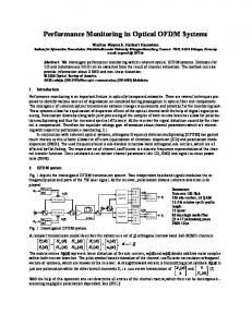
OFDM Channel Gain Vector g=[g1,…,gK]T Info. bits

k=1 T

r*(c)=[r1*,…,rK*]

OFDM Mod

OFDM Demod

k=K

p*(c)=[p1*,…,pK* ]T

Transmission Mode Control

Fig. 1.

Channel Estimation g Finite Rate Feedback Control Link ĺl og2(c) bits

Q-CSI c(g)

Resource Allocation

System block diagram.

initialization (off-line) phase and requires a negligible burden during the transmission (online) phase, which is certainly welcome from an implementation perspective. The minimization of the average transmit-power in a setup with multiple users under more restrictive conditions than those in this paper has been recently investigated in [17]. With an eye on practicality, together with the optimal schemes we are also interested in algorithms with small computational burden. We will propose new simplified designs and adapt others existing in the literature ([7], [17], [18], [19]), giving rise to reduced-complexity schemes whose performance is very close to the optimal one. To achieve these goals, we will rely on optimization theory, vector quantization, and stochastic approximation tools. The rest of the paper is organized as follows. After introducing preliminaries on the setup (Section II), we formulate the average rate-efficient OFDM optimization problem based on LRF and derive optimality conditions for the channel quantizer and power and rate loading policies (Section III). Suboptimal schemes that reduce the computational complexity required for both designing the channel quantizer and the power and rate loadings (Section IV) are also investigated. Different strategies aiming at reducing the amount of feedback required to implement the adaptive schemes are reviewed (Section V), and several issues regarding practical implementation are briefly discussed (Section VI). Numerical results and comparisons that corroborate our claims are presented (Section VII), and concluding remarks wrap up this paper (Section VIII).1 II. P RELIMINARIES As illustrated in Fig. 1, we consider wireless OFDM transmissions over 𝐾 subcarriers through frequency-selective 1 Notation: Lower and upper case boldface letters are used to denote (column) vectors and matrices, respectively; (⋅)𝑇 denotes transpose; [⋅]𝑘,𝑙 the (𝑘, 𝑙)th entry of a matrix, and [⋅]𝑘 the 𝑘th entry of a vector; X ≥ 0 means all entries of X are nonnegative; F𝑁 stands for the normalized FFT 2𝜋 matrix with entries [F𝑁 ]𝑛,𝑘 = 𝑒−𝑗 𝑁 𝑘𝑛 , 𝑛, 𝑘 = 0, . . . , 𝑁 − 1; 𝑓X (X) denotes the joint probability density function (PDF) of matrix X; likewise, 𝑓𝑥 (𝑥) denotes the PDF of a scalar 𝑥; 𝔼X [⋅] stands for the expectation operator over X; ⌊⋅⌋ (⌈⋅⌉) denotes the floor (ceiling) operation; 𝑥∗ the optimal value of variable 𝑥; and [𝑥]+ stands for max(0, 𝑥).

fading channels with discrete-time baseband equivalent impulse response taps {ℎ𝑛 }𝑁 𝑛=0 , where 𝑁 denotes the channel order (i.e., the maximum delay spread divided by the time symbol is equal to 𝑁 ). Initially, a serial stream of data bits is de-multiplexed to form 𝐾 parallel streams indexed by 𝑘 = 1, . . . , 𝐾. Defining p and r as non-negative 𝐾 × 1 vectors, the 𝑘th stream is next multiplied by a constant to load instantaneous power [p]𝑘 , and properly coded and modulated to give rise to an instantaneous transmit rate [r]𝑘 . Once the proper set of operations are performed at both transmitter and receiver sides (Fast Fourier Transform -FFT-, cyclic prefix, multiplexing, digital to analog conversion, etc.), the multipath fading frequency-selective channel is converted into a set of 𝐾 parallel flat-fading subchannels each with fading by the FFT (see e.g., [1]): 𝐻𝑘 = √ coefficient ∑𝐾−1 given 2𝜋 (1/ 𝐾) 𝑛=0 ℎ𝑛 𝑒−𝑗 𝐾 𝑘𝑛 , where 𝐾 is typically chosen so that 𝐾 ≫ 𝑁 . Channel estimation at the receiver relies on periodically inserted training symbols. When the channel is estimated, the receiver has available a noise-normalized chan2 𝑇 ] , where 𝜎𝑘2 nel gain vector g := [∣𝐻1 ∣2 /𝜎12 , . . . , ∣𝐻𝐾 ∣2 /𝜎𝐾 is the variance of the zero-mean additive white Gaussian noise (AWGN) in the 𝑘th subcarrier. While each realization of the gain vector g constitutes the P-CSI, in Q-CSI approaches the domain of g is divided into 𝐿 different regions {퓡𝑙 }𝐿 𝑙=1 and only the specific region where the current channel realization falls into is known. Different criteria have been proposed in the literature for efficiently defining these regions, some of which will be later summarized. Once the criterion is selected, the corresponding {퓡𝑙 }𝐿 𝑙=1 can be obtained and sent to both transmitter and receiver. After that point, only an index identifying the active region needs to be fed back from the receiver to the transmitter. Defining 𝐵 := ⌈log2 (𝐿)⌉, we denote by c = c(g) the 𝐵 × 1 vector of bits used as the index of the region the current channel realization falls into. Clearly, c is the piece of information that must be fed back from the receiver to the transmitter in Q-CSIT based OFDM schemes. The ultimate goals of this paper are to properly design a channel quantizer to obtain c; and given c(g), to find the appropriate allocation (loading) vectors p(c) and r(c). Since c can take 𝐿 different values (one per region), 𝐿 different power and rate loadings need to be designed. Specifically, r𝑙

3132


and p𝑙 are used to denote, respectively, the non-negative 𝐾 ×1 rate and power vectors to be loaded when the 𝑙th region is active (i.e., when g ∈ 퓡𝑙 ). It is important to emphasize that so far no structure, neither for the channel quantizer nor for the rate-power codebook, has been assumed. With an eye on practicality, Sections IV and V will discuss low complexity quantizers which presume an underlying structure. To proceed with the design, the following assumptions will be considered: (as1) Regions remain invariant over at least two consecutive OFDM symbols. (as2) The feedback channel is error-free and incurs negligible delay. (as3) The instantaneous BER function per subcarrier denoted by 𝜖([p]𝑘 , [r]𝑘 , [g]𝑘 ) is jointly convex with respect to (w.r.t.) [p]𝑘 and [r]𝑘 . Assumption (as1) allows each subchannel to vary from one OFDM symbol to the next so long as the quantization region in which it falls remains invariant; error-free feedback under assumption (as2) is easily guaranteed with sufficiently strong error control codes, especially since data rates in the feedback link are typically low; and assumption (as3) will help the development of efficient algorithms and holds for many practical situations. An example of BER function satisfying (as3) is ( ) 𝜖([p]𝑘 , [r]𝑘 , [g]𝑘 ) =𝜅1 exp −𝜅2 [p]𝑘 [g]𝑘 /(2[r]𝑘 − 1) , (1) [g]𝑘 > (2[r]𝑘 − 1)/[p]𝑘 ; where the constants 𝜅1 and 𝜅2 depend on the specific modulation and code implemented. The accuracy of (1) for (un)coded QAM modulations is widely accepted; see, e.g., [20]. III. O PTIMAL D ESIGN A. Problem Formulation The first step to formulate the optimization problem is to find the expressions for the average transmit-rate 𝑟¯ and transmit-power 𝑝¯ over all subcarriers. Since p𝑙 and r𝑙 are2 the instantaneous power and rate values that the system will load when g ∈ 퓡𝑙 , the expressions for 𝑟¯ and 𝑝¯ are: 𝑟¯

:= =

𝑝¯

:= =

𝐾 ∑

𝔼g [[r𝑙(g) ]𝑘 ] =

𝑘=1 𝐿 𝐾 ∑ ∑ 𝑘=1 𝑙=1 𝐾 ∑

𝔼g∈퓡𝑙 [[r𝑙 ]𝑘 ] Pr{g ∈ 퓡𝑙 }

𝑘=1 𝑙=1

[r𝑙 ]𝑘 Pr{g ∈ 퓡𝑙 }

𝔼g [[p𝑙(g) ]𝑘 ] =

𝑘=1 𝐾 ∑ 𝐿 ∑

𝐿 𝐾 ∑ ∑

𝐿 𝐾 ∑ ∑ 𝑘=1 𝑙=1

[p𝑙 ]𝑘 Pr{g ∈ 퓡𝑙 }.

power transmitted on subcarrier 𝑘, [p𝑙 ]𝑘 ≤ 𝑝max . Note that the 𝑘 constraint is different for each 𝑘 because spectral masks may vary depending on the frequency of operation. Moreover, we also impose a maximum average BER ¯𝜖0 for our system, and for this purpose, the average BER per subcarrier3 and region needs to satisfy 𝔼g∈퓡𝑙 [𝜖([p𝑙 ]𝑘 , [r𝑙 ]𝑘 , [g]𝑘 )] ≤ ¯𝜖0 ∀𝑘, 𝑙. Analytically, the constrained optimization problem we aim to solve is: ⎧  max 𝑟¯,   {ˇ p𝑙 },{r𝑙 },{퓡𝑙 }    subject to : 𝐶1. ⎨ 𝐶2.     𝐶3.    ⎩ 𝐶4.

∑𝐾 where 𝑟¯ := 𝑘=1 𝔼g [[r𝑙(g) ]𝑘 ] ∑𝐾 ¯0 , 𝑘=1 𝔼g [[p𝑙(g) ]𝑘 ] ≤ 𝑝 𝔼g∈퓡𝑙 [𝜖([p𝑙 ]𝑘 , [r𝑙 ]𝑘 , [g]𝑘 )] ≤ 𝜖¯0 , ∀𝑘, 𝑙, 0 ≤ [p𝑙 ]𝑘 ≤ 𝑝max , ∀𝑘, 𝑙 𝑘 [r𝑙 ]𝑘 ≥ 0, ∀𝑘, 𝑙. (4) The objective in (4) is to maximize the average rate over all possible channel realizations. However, the constraints involve different forms of CSI: 𝐶1 is an average requirement; 𝐶2 pertains to an average per region; 𝐶3−𝐶4 need to be satisfied per region 𝑙 and subcarrier 𝑘. Even though constraint 𝐶1 ensures that the average power does not exceed 𝑝¯0 , it does not impose any limit on the power transmitted ∑instantaneous 𝐾 during an OFDM symbol, 𝑘=1 [p𝑙(g) ]𝑘 , which is allowed to vary in time. As for the instantaneous upper bound in 𝐶3, it imposes power spectral mask constraints in every region. In the following subsection, we will derive the KarushKuhn-Tucker (KKT) conditions associated with (4). These will not only lead us to the expressions determining the optimal loading variables but will also provide valuable insights on the structure of the rate-efficient resource allocation policies. But before presenting the KKT conditions, the following remark on the formulation of the optimization problem is in order. Remark 1: Optimization throughout this paper is carried out for continuous-rate (CR) loadings. Although the hardware complexity for implementing CR modulation and coding schemes is higher than the required for discrete-rate (DR) loadings [20], optimizing CR loadings is analytically more convenient and leads to a higher rate efficiency. Furthermore, for systems that implement DR loadings, the CR solution not only offers intuition and useful guidelines for the DR design, but also can be transformed into a a DR loading using algorithms available in the literature; see, e.g., [21].

(2) 𝔼g∈퓡𝑙 [[p𝑙 ]𝑘 ] Pr{g ∈ 퓡𝑙 } B. Optimality Conditions (3)

𝑘=1 𝑙=1

Our goal is to maximize 𝑟¯, subject to an average power constraint. Specifically, we want to constrain the average power across all subcarriers, i.e., 𝑝¯ ≤ 𝑝¯0 . Additionally, to put into practice power spectral masks we constrain the instantaneous 2 The subscript 𝑙 here will be also written explicitly as 𝑙(g) in places that this dependence must be emphasized.

We will start by considering the optimization problem (4) constrained to 𝐶1 and 𝐶2 alone, and then include constraints 𝜖 denote the non-negative Lagrange 𝐶3 and 𝐶4. Let 𝛽 𝑝 and 𝛽𝑘,𝑙 multipliers associated with 𝐶1 and 𝐶2, respectively. The 3 The latter constraint is imposed for every subcarrier because: i) it will reduce the coupling among the variables to optimize and ii) it will not entail a significant loss of optimality (see, e.g., [17] for additional comments on this issue).


∑ ∑𝐾 ∑ 𝑝 𝜖 ¯0 + 𝐿 ¯0 ), where ( 𝐿 𝑙=1 𝔼g∈퓡𝑙 {𝜑𝑙 (g)}) + (𝛽 𝑝 𝑙=1 𝑘=1 𝛽𝑘,𝑙 𝜖 the second term does not depend on 퓡𝑙 . It is clear then that in order to maximize ℒ, each channel realization g has to be assigned to the region which entails a higher reward, yielding

Lagrangian of (4) can be written as: 𝜖 }, {p𝑙 }, {r𝑙 }, {퓡𝑙 }) = ℒ(𝛽 𝑝 , {𝛽𝑘,𝑙 (𝐾 ) 𝐾 ∑ ∑ 𝑝 𝔼g [[r𝑙(g) ]𝑘 ] − 𝛽 𝔼g [[p𝑙(g) ]𝑘 ] − 𝑝¯0 𝑘=1 𝐿 𝐾 ∑ ∑

−

(5)

𝑘=1 𝜖 𝛽𝑘,𝑙 (𝔼g∈퓡𝑙 [[r𝑙 ]𝑘 𝜖([p𝑙 ]𝑘 , [r𝑙 ]𝑘 , [g]𝑘 )] − 𝜖¯0 ) .

𝑘=1 𝑙=1

Based on the previous notation, the KKT conditions associated with the rate and power loadings dictate that at the optimal solution (remember that 𝑥∗ denotes the optimal value of 𝑥): Pr{g ∈ 퓡∗𝑙 } 𝜖∗ 𝔼g∈퓡∗𝑙 − 𝛽𝑘,𝑙

[

] ∂𝜖([p∗𝑙 ]𝑘 , [r∗𝑙 ]𝑘 , [g]𝑘 ) = 0, ∂[r𝑙 ]𝑘

− 𝛽 𝑝∗ Pr{g ∈ 퓡∗𝑙 } [ ] ∂𝜖([p∗𝑙 ]𝑘 , [r∗𝑙 ]𝑘 , [g]𝑘 ) 𝜖∗ ∗ − 𝛽𝑘,𝑙 𝔼g∈퓡𝑙 = 0, ∂[p𝑙 ]𝑘

∀𝑘, 𝑙,

∀𝑘, 𝑙.

(6)

(7)

𝜖∗ Note that if 𝛽 𝑝∗ , 𝛽𝑘,𝑙 and 퓡∗𝑙 , were known, [r∗𝑙 ]𝑘 and [p∗𝑙 ]𝑘 could be easily found using an ellipsoid search (remember that the BER in convex w.r.t. the power and rate loadings, so that the derivatives in (6) and (7) are monotonic). On the and other hand, 𝐶3 and 𝐶4 impose that 0 ≤ [p𝑙 ]𝑘 ≤ 𝑝max 𝑘 [r𝑙 ]𝑘 ≥ 0 ∀(𝑙, 𝑘). Even though it can be rigorously deduced from the KKT conditions associated with 𝐶3 and 𝐶4, it is not difficult to see that if the solution of (6) and (7) does not satisfy the requirements in 𝐶3 and 𝐶4, in order to find the optimal feasible solution it suffices to project the unfeasible solution into the constrained set (e.g., by setting to zero negatives entries of r∗𝑙 and p∗𝑙 ). The KKT conditions associated with 𝐶1 and 𝐶2 (also known as complementary slackness conditions [22]) dictate that (𝐾 ) ∑ 𝑝∗ ∗ 𝛽 × 𝔼g [[p𝑙(g) ]𝑘 ] − 𝑝¯0 = 0 (8) 𝑘=1 ( ) 𝜖∗ × 𝔼g∈퓡∗𝑙 [𝜖([p∗𝑙 ]𝑘 , [r∗𝑙 ]𝑘 , [g]𝑘 )] − 𝜖¯0 = 0 ∀𝑘, 𝑙. 𝛽𝑘,𝑙

(9)

In words, the optimum solution is such that either the constraints are met with equality or the corresponding Lagrange multipliers are zero. It is not difficult to show that if ∑ 𝐾 max > 𝑝¯0 , then the optimum Lagrange multipliers 𝛽 𝑝∗ 𝑘=1 𝑝𝑘 𝜖∗ and {𝛽𝑘,𝑙 } are non-zero and therefore the constraints in 𝐶1 and 𝐶2 are met with equality. In order to obtain the optimal quantization regions, we capitalize on the separable structure of the Lagrangian in (5). This can be done without assuming any a priori structure for the quantization regions. First, let us define the reward 𝜑∗𝑙 (g) of assigning realization g to region 𝑙 as 𝜑∗𝑙 (g) := −

𝐾 ∑

[r∗𝑙(g) ]𝑘 − 𝛽 𝑝∗

𝑘=1 𝐾 ∑

𝐾 ∑

3133

[p∗𝑙(g) ]𝑘

𝑘=1

(10)

𝜖∗ 𝛽𝑘,𝑙 𝜖([r∗𝑙(g) ]𝑘 , [p∗𝑙(g) ]𝑘 , [g]𝑘 ).

𝑘=1

Additionally, using the definition in (10), the Lagrangian can be decomposed across channel realizations and regions as ℒ =

퓡∗𝑙 = {g : 𝜑∗𝑙 (g) > 𝜑∗𝑙′ (g) ∀𝑙′ ∕= 𝑙},

∀𝑙.

(11)

More, since 𝜑∗𝑙 (g) is monotonic w.r.t. [g]𝑘 (and this is true because the BER is strictly decreasing w.r.t. [g]𝑘 ), the optimal regions in (11) can be equivalently represented by continuous boundaries in the g domain (ℝ𝐾 ). Therefore, in order to decide in which region a channel realization g falls into, the reward in (10) is evaluated for every 𝑙 and the the region is selected according to (11), so that the reward is maximized. Note that to carry out this task, there is no need for defining any quantization region structure, 𝜖∗ 𝐾 but instead, only the values of p∗𝑙 , r∗𝑙 and {𝛽𝑘,𝑙 }𝑘=1 ∀𝑙 are required. It is worth emphasizing that the definition of 𝜑𝑙 (g) has not been previously assumed, but instead it emerged from the Lagrangian of (4). In other words, the regions in (11) have been derived from the generic optimization problem. This is a significant difference from most works in the literature, where either the structure for the channel quantizer, or the value of 퓡𝑙 itself, are assumed beforehand. C. Finding a Local Optimum Since the problem in (4) is not convex, KKT conditions are necessary but not sufficient. This implies that to find the overall global optimum, all the solutions of (6)-(11) have to be found and then the one that achieves the higher average transmitted rate 𝑟¯ needs to be selected. Unfortunately, from a complexity perspective there is not an efficient way to find all the solutions of (6)-(11). In fact (4) can be cast as a vector constrained quantization problem, which is highly non-convex and typically NP-hard [23]. An approach to deal with quantization problems is to implement a block coordinate ascend method [24], which is a method widely used to find local optimums of non-convex problems. The block coordinate ascend method proceeds into two phases. First, the values of some variables (here regions) are considered to be given and based on them, the values of the remaining variables (here rate and power) are found. Second, the values of the updated variables (rate and power) are considered to be given and based on them, the values of the remaining variables (regions) are optimally found. If these two phases are iterated, convergence to a stationary point is guaranteed. Had the constraints in (4) not been present, this method would correspond to the well-known Lloyd Algorithm [25] with a distortion metric −¯ 𝑟 (the minus sign is because here we aim to maximize 𝑟¯, which amounts to minimize −¯ 𝑟). Several options are possible to account for the constraints in (4). One of them is to use the −ℒ in (5) as a distortion metric; see, e.g., [8], [17]. The major drawback of this approach is that an exhaustive (𝐾𝐿 + 1) dimensional search to find the Lagrange multipliers has to be implemented. Another option is to satisfy the constraints at every phase of the ascend method. This way, at every iteration two phases are implemented: a) in phase 𝐿 1, problem in (4) is solved w.r.t. {p𝑙 }𝐿 𝑙=1 and {r𝑙 }𝑙=1 with

3134


{퓡𝑙 }𝐿 𝑙=1 given from the previous iteration and b) in phase 𝐿 2, problem in (4) is solved w.r.t. {퓡𝑙 }𝐿 𝑙=1 with {p𝑙 }𝑙=1 and 𝐿 {r𝑙 }𝑙=1 given from phase 1. The problem in phase 1 is convex and therefore, easy to solve. However, a major drawback of this option is that problem in phase 2 is still non-convex and difficult to solve. To find a point satisfying the KKT conditions without incurring a high computational complexity, we propose next a modified version of the latter algorithm. The main idea is that the optimum calculation of the quantization regions in phase 2 is replaced with the optimality conditions in (10) and (11). To be specific, during phase 1, the regions are considered fixed and problem in (4) is solved only w.r.t. power and rate loadings using a dual approach. During phase 2, the rates, powers, and Lagrange multipliers obtained in phase 1 are substituted into (10) and (11) to get the quantization regions. Phase 1 and phase 2 are iterated until convergence occurs. If the previous algorithm converges (which is not always guaranteed), it will converge to a point satisfying the KKT conditions. Note also that the complexity of each of the phases is small since problem in phase 1 is convex and problem in phase 2 is solved using (10) and (11). Regarding the solution of the problem in phase 1, it is important to keep in mind that a dual method has to be used. This is because the Lagrange multipliers are needed to obtain the channel quantizer using (10) and (11). The literature provides different methods that numerically search for the optimal values of the Lagrange multipliers. A successful one is the method of the multipliers [24], which relies on the fact that constraints 𝐶1 and 𝐶2 are always active and 𝜖 are calculated so that the constraints therefore 𝛽 𝑝 and 𝛽𝑘,𝑙 are satisfied as equality. For the problem at hand, if 𝜷 := 𝜖 𝜖 𝜖 𝜖 [𝛽 𝑝 , 𝛽1,1 , 𝛽1,2 , . . . , 𝛽𝐾,𝐿−1 , 𝛽𝐾,𝐿 ]𝑇 denotes a (𝐾𝐿 + 1) × 1 vector collecting all the Lagrange multipliers, 𝑖 stands for iteration index, and 𝜇(𝑖) represents a non-increasing step-size, then the Lagrange multipliers are updated in the form 𝜷(𝑖 + 1)𝑇 = [𝜷(𝑖)𝑇 + 𝜇(𝑖)Δ(𝜷(𝑖))𝑇 ]+ ;

(12)

where each entry of Δ(𝛽(𝑖)) corresponds to the violation of the respective constraint when 𝜷(𝑖) is used as the optimum value of the Lagrange multipliers, i.e. [Δ(𝜷 ∗ )]𝑛 =

𝐾 ∑

𝔼g [[p𝑙(g) (𝜷 ∗ )]𝑘 ] − 𝑝¯0 ,

𝑛 = 1,

(13)

𝑘=1

[Δ(𝜷∗ )]𝑛 = 𝔼g∈퓡𝑙 [𝜖 ([p𝑙 (𝜷 ∗ )]𝑘 , [r𝑙 (𝜷 ∗ )]𝑘 , [g]𝑘 )] − ¯𝜖0 , 𝑛 = (𝑘 − 1)𝐿 + 𝑙 + 1. (14) We refer the reader to [24, Chapter 4] for a more detailed explanation of this method. It can be shown that for a broad range of stepsizes the iteration in (12) converges to a point for which the constraints are satisfied with equality (which is the overall global optimum if the original problem is strictly convex). According to this discussion, we next outline the steps of an algorithm that can be implemented to find a feasible yet suboptimum solution.

Algorithm 1: Joint Resource Allocation and Quantization (JRAQ) (S1.0) Let 𝑖 be an iteration number, 𝐼 be the maximum number of iterations. For 𝑖 = 0, start with arbitrary regions 퓡𝑙 (𝑖) and then set 𝑖 = 1. (S1.1) Let 𝑗 be an iteration number. For 𝑗 = 0, start with small 𝜖 (𝑖, 𝑗) and keep 𝑗 = 0: multipliers 𝛽 𝑝 (𝑖, 𝑗) and 𝛽𝑘,𝑙 𝜖 (S1.1.1) Substitute 퓡𝑙 (𝑖), 𝛽 𝑝 (𝑖, 𝑗) and 𝛽𝑘,𝑙 (𝑖, 𝑗) into (6)-(7) to ∗ ∗ ∗ find p𝑙 and r𝑙 ∀𝑙. Set p𝑙 (𝑖, 𝑗) = p𝑙 and r𝑙 (𝑖, 𝑗) = r∗𝑙 . (S1.1.2) Use p𝑙 (𝑖, 𝑗) and r𝑙 (𝑖, 𝑗) to check constraints 𝐶1 and 𝐶2 in (4). If ∣𝐶1∣ ≈ 0 and ∣𝐶2∣ ≈ 0 then stop, set p𝑙 (𝑖) = p𝑙 (𝑖, 𝑗), r𝑙 (𝑖) = r𝑙 (𝑖, 𝑗), 𝛽 𝑝 (𝑖) = 𝛽 𝑝 (𝑖, 𝑗) and 𝜖 𝜖 𝛽𝑘,𝑙 (𝑖) = 𝛽𝑘,𝑙 (𝑖, 𝑗), and go to (S1.2). Otherwise, update 𝜖 𝛽 𝑝 (𝑖, 𝑗) and 𝛽𝑘,𝑙 (𝑖, 𝑗) according to (12), increase 𝑗 and go to (S1.1.1). 𝜖 (𝑖) into (10) and (11) to (S1.2) Substitute p𝑙 (𝑖), r𝑙 (𝑖), 𝛽 𝑝 (𝑖), and 𝛽𝑘,𝑙 ∗ ∗ find 퓡𝑙 ∀𝑙. Set 퓡𝑙 (𝑖) = 퓡𝑙 . 𝜖 (𝑖) to p𝑙 (𝑖 − 1), r𝑙 (𝑖 − 1), (S1.3) Compare p𝑙 (𝑖), r𝑙 (𝑖), 𝛽 𝑝 (𝑖), and 𝛽𝑘,𝑙 𝜖 𝛽 𝑝 (𝑖 − 1), and 𝛽𝑘,𝑙 (𝑖 − 1). If the difference is small or if 𝑖 = 𝐼, then stop and go to (S1.4) ; otherwise increase 𝑖, and go to (S1.1). 𝐿 (S1.4) If 𝑖 = 𝐼, then return {p𝑙 (𝑖)}𝐿 𝑙=1 , {r𝑙 (𝑖)}𝑙=1 and {퓡𝑙 (𝑖 − 𝐿 𝐿 as solution. Otherwise, return {p (𝑖)} 1)}𝐿 𝑙 𝑙=1 𝑙=1 , {r𝑙 (𝑖)}𝑙=1 𝐿 and {퓡𝑙 (𝑖)}𝑙=1 as solution

Note that step (S1.4) is required because {퓡𝑙 (𝑖)}𝐿 𝑙=1 in (S1.3) may fail to satisfy the constraints in (4). As mentioned, convergence of the above algorithm is not guaranteed and depends critically on the initialization steps (standard approaches to deal with this problem include finding a good initial point and/or using multiple initializations). Remarkably, since the 𝐿 problem in (4) is jointly convex w.r.t. {p𝑙 }𝐿 𝑙=1 and {r𝑙 }𝑙=1 , it holds that the power and rate loadings returned by Algorithm 1 are globally optimum if the channel quantizer is fixed beforehand. This feature will be further exploited in the next section to reduce the complexity of the overall design. From an operational perspective, the dynamic resource allocation based on Q-CSI proceeds as follows. During an initialization phase the receiver runs Algorithm 1; finds {p∗𝑙 }𝐿 𝑙=1 , ∗ 𝐿 ∗ 𝐿 ∗ 𝐿 {r∗𝑙 }𝐿 and {퓡 } ; and feeds {p } and {r } back 𝑙 𝑙=1 𝑙=1 𝑙 𝑙=1 𝑙 𝑙=1 to the transmitter (note that if the transmitter also runs Algorithm 1, then there is no need of feeding back the optimal rate and power codebooks during the initialization phase). Once the system has been initialized, during the transmission phase the following two actions have to be taken every time the channel changes (i.e., every coherence interval). First, the receiver estimates g, relies on {퓡𝑙 }𝐿 𝑙=1 to find the index of the region the current channel realization belongs to, codifies that index into the codeword c, and feeds back that codeword to the transmitter. Second, the transmitter decodes c and selects the corresponding p𝑙 and r𝑙 vectors that are loaded during the current coherence time. As pointed out in the introduction, different from, e.g. [26] or [7], the average formulation in (4) leads to an online phase with negligible computational complexity, which is certainly of interest in most dynamic wireless systems. Since there is no scheme that for any instance of the problem is able to find p∗𝑙 , r∗𝑙 and 퓡∗𝑙 in polynomial time, from an implementation perspective we always have to shoot for suboptimal schemes. In the next section different simplifications in the formulation will be proposed, giving rise to schemes with a low-complexity initialization (off-line) phase. As it will


be shown, those schemes will be guaranteed to converge and yield an overall performance very close to the optimal. IV. R EDUCED -C OMPLEXITY A LGORITHMS In this section, reduced-complexity quantization and resource allocation algorithms which entail a small loss of optimality (average rate performance) are designed. To do so we will try to simplify the main tasks carried out in Algorithm 1. Specifically three simplifications are investigated. First, we consider a non iterative channel quantizer that quantizes each subcarrier separately and gives rise to a convex design. Second, we propose a robust worst-case design that greatly reduces the dimensionality of the novel resource allocation problem. Third, using stochastic approximation tools, we propose a low-complexity stochastic iteration that estimates the value of the Lagrange multipliers on-the-fly and eliminates the need of running an algorithm during the initialization phase. For all cases, the loss of performance due to the simplifications here considered will be numerically evaluated through simulations in Section VII. A. Fixed Scalar (Per Subcarrier) Quantizer So far no prior structure of the channel quantizer was assumed and a generic vector quantizer has been obtained in (10) and (11). Since the entries of g are positive real numbers, a popular low-complexity alternative quantizer consists of performing separate scalar quantization of each of the entries of g [10], [7], [17]. This alternative not only is desirable from an implementation perspective (scalar quantizers are inexpensive and widely spread), but also entails a reduction of the complexity required to implement resource allocation algorithms. Furthermore, numerical results will corroborate that for medium-high feedback rates, this assumption does not entail a significant loss of performance. Based on this, we can suppose that: (as.4) A realization of each [g]𝑘 gain falls into one of 𝐿𝑘 𝑘 disjoint regions {ℛ𝑘,𝑙 }𝐿 𝑙=1 . Under (as.4) the domain of the 𝑘th entry of vector g is divided into 𝐿𝑘 regions, and therefore the number of regions 𝐿 in which the domain of the entire vector g is divided is 𝐿 = Π𝐾 𝑘=1 𝐿𝑘 . Furthermore, since the BER is a monotonic function w.r.t. [g]𝑘 , it can be concluded that without loss of optimality, each of those 𝐿𝑘 regions can be described by a single interval ℛ𝑘,𝑙 = [𝜏𝑘,𝑙−1 , 𝜏𝑘,𝑙 ) with 𝜏𝑘,0 = 0 and 𝜏𝑘,𝐿𝑘 = ∞. As a result the scalar subcarrier quantizer can be alternatively described 𝑘 using 𝐿𝑘 + 1 different quantization thresholds {𝜏𝑘,𝑙 }𝐿 𝑙=0 . With regard to the design of resource allocation schemes, (as.4) typically entails that the power and rate loadings corresponding to the lowest regions are zero. This is because the realizations in [0, 𝜏𝑘,1 ) are so poor that the power required to attain a medium-low BER is so high that the best decision is not to transmit. 1) Equally Probable Region Quantizer: As it was explained before, algorithms in Section III-C cannot yield the optimal global solution of problem (4). The underlaying reason is that the original problem in (4) is not convex w.r.t. {퓡𝑙 }. As a result, the regions returned by those algorithms are

3135

typically local optima that heavily depend on the initialization. Nevertheless, since the problem in (4) is jointly convex w.r.t. {p𝑙 } and {r𝑙 }, if the regions were fixed, then the power and rate loadings obtained in step (S1.1) of Algorithm 1 would be globally optimal. Although (as.4) reduces the complexity of the design, finding the optimum scalar quantizer is still a nonconvex problem. This prompt us to propose a low-complexity non-iterative procedure where the quantization regions are designed beforehand under a reasonable alternative criterium and the optimal power and rate loadings are obtained running a single iteration of step (S1.1) in Algorithm 1 (without a need of implementing a coordinate ascent approach). Among several available alternatives to design the noniterative scalar channel quantizer, we select the equallyprobable region quantizer in [7, Sec. V-B.2.a]. The motivation for selecting this quantizer is three-fold: i) in many cases a closed-form solution for the channel thresholds is available; ii) from an optimality perspective, this quantizer maximizes the entropy of the Q-CSI corresponding to a single subcarrier; and iii) extensive numerical simulations have shown that loss of performance relative to the optimum scalar quantizer is small even for low feedback rates. Specifically, the equally-probable region quantizer determines 𝜏𝑘,𝑙 ’s so that ∫ Pr(𝑔𝑘 ∈ ℛ𝑘,𝑙 ) =

𝜏𝑘,𝑙+1

𝜏𝑘,𝑙

𝑓𝑔𝑘 (𝑔𝑘 )𝑑𝑔𝑘 = 1/𝐿𝑘 ∀(𝑘, 𝑙). (15)

For Rayleigh channels (where subcarrier gains adhere to exponential PDF’s), (15) yields the following closed-form solution 𝜏𝑘,𝑙 = 𝑔¯𝑘 ln (𝐿𝑘 /(𝐿𝑘 − 𝑙)).

(16)

Unless explicitly mentioned, in the remaining sections the equally probable region quantizer will be implemented.

B. Robust Worst-Case Design Instead of maximizing 𝑟¯, in this section we will maximize 𝑟ˇ, a lower bound on 𝑟¯∗ . Maximizing a lower bound is a commonly used technique when direct optimization of the original objective function is difficult [24]. To this end, let 𝜖−1 𝑟 denote the inverse function involved when solving (1) w.r.t. the rate loading, and [g𝑙min ]𝑘 := min{[g]𝑘 ∣ g ∈ 퓡𝑙 } represent the worst channel gain for the specific ∑ (𝑙, 𝑘) pair. Then we can r𝑙(g) ]𝑘 ], where lower bound 𝑟¯ in (4) using 𝑟ˇ := 𝐾 𝑘=1 𝔼g [[ˇ min ]𝑘 , 𝜖¯0 ). [ˇ r𝑙 ]𝑘 := 𝜖−1 𝑟 ([p𝑙 ]𝑘 , [g𝑙

(17)

Note that if the scalar quantizer presented in Section IV-A is implemented, then [g𝑙min ]𝑘 = 𝜏𝑘,𝑙−1 . The design parameters using this lower bound approach will be identified with the superscript “∨ ”. The lower bound in (17) brings the following advantages: i) constraint 𝐶2 is automatically satisfied and thus 𝜖 = 0 ∀𝑘, 𝑙, and ii) a direct link is established between [p𝑙 ]𝑘 𝛽𝑘,𝑙 and [r𝑙 ]𝑘 through 𝜖−1 𝑟 and therefore we need only to optimize over either variable, thus reducing the dimensionality.

3136


With rate variables eliminated, the new optimization prob- (S2.1) Substitute 𝛽ˇ𝑝 (𝑖) into (19) to find p ˇ ∗𝑙 ∀𝑙. Set p𝑙 (𝑖) = p ˇ ∗𝑙 . ˇ ˇ (S2.2) Use p (𝑖) to check constraint 𝐶 1 in (18). If ∣𝐶 1∣ < 𝛿𝑝0 then 𝑙 lem is expressed as: stop and go to (S2.3); otherwise update 𝛽ˇ𝑝 (𝑖) according to (20), ⎧ ∑𝐾 min increase 𝑖 and go to (S2.1).  max 𝑟ˇ, where 𝑟ˇ := 𝑘=1 𝔼g [𝜖−1 p𝑙(g) ]𝑘 , [g𝑙(g) ]𝑘 , 𝜖¯0 )]  𝑟 ([ˇ ⎨ {ˇp𝑙 } (S2.3) Substitute p𝑙 (𝑖) into (17) (robust design) or into (22) (tight ∑𝐾 design) to find the final rate loadings. Return {ˇ p𝑙 (𝑖)}𝐿 p𝑙(g) ]𝑘 ] ≤ 𝑝¯0 , subject to : 𝐶 ˇ 1. 𝑙=1 and 𝑘=1 𝔼g [[ˇ  𝐿 𝐿  ⎩ r𝑙 (𝑖)}𝑙=1 ) as the optimal solution. {ˇ r𝑙 (𝑖)}𝑙=1 (or {˜ max ˇ ∀(𝑘, 𝑙). 𝐶 3. 0 ≤ [ˇ p 𝑙 ]𝑘 ≤ 𝑝 𝑘 (18) The optimization in (18) can be easily cast as a convex As in the case of Algorithm 1, Algorithm 2 is run off-line problem, whose optimal solution will be denoted by p ˇ∗𝑙 . If during an initialization phase. Once the optimal power and 𝐶ˇ 3 is ignored, then the KKT conditions (which for (18) are rate loadings for all the regions are known, the transmitter necessary and sufficient) associated with the power loadings will use c to load the optimal p r𝑙 (˜ r𝑙 ) corresponding to ˇ𝑙 and ˇ are: the region that c indexes. p∗𝑙 ]𝑘 , [g𝑙min ]𝑘 , 𝜖¯0 ) ˇ𝑝∗ ∂𝜖−1 𝑟 ([ˇ − 𝛽 = 0, ∀(𝑘, 𝑙). (19) C. Stochastic Computation of the Optimum Lagrange Multi∂[ˇ p 𝑙 ]𝑘 pliers The optimal powers in (19) can be found using an oneThe main burden of Algorithm 2 is associated with the dimensional search. Note that if after solving (19) the optimum computation of 𝛽ˇ𝑝∗ . As mentioned before, Algorithm 2 is ˇ powers do not satisfy 𝐶 3, the optimum feasible powers can be found by projecting each of the solutions of (19) onto the performed off-line and requires knowledge of the channel statistics. In fact, to evaluate Δ(𝛽ˇ𝑝 (𝑖)) in (S2.2), the value ] interval [0, 𝑝max 𝑘 Regarding the optimal value of 𝛽ˇ𝑝∗ , a similar approach to of 𝑝¯ needs to be computed. According to (3), this implies the one developed in Section III-C can be used to find the that the probabilities Pr{g ∈ 퓡𝑙 } have to be known for every 𝑙. However there are situations where this computation optimal value of the multiplier through the iteration cannot be efficiently carried out or is not even feasible. For [ ] ˇ 𝛽ˇ𝑝 (𝑖)) + , (20) example: in scenarios where the setup (channel distribution, 𝛽ˇ𝑝 (𝑖 + 1) = 𝛽ˇ𝑝 (𝑖) + 𝜇(𝑖)Δ( 𝐾 QoS requirements) changes so frequently so that 𝛽ˇ𝑝∗ has to be ∑ 𝑝∗ 𝑝∗ ˇ ˇ ˇ Δ(𝛽 ) = 𝔼g [[ˇ p𝑙(g) (𝛽 )]𝑘 ] − 𝑝¯0 . (21) continuously re-computed, in limited-complexity systems that 𝑘=1 cannot afford the off-line burden (for systems with high 𝐾, the Different from Section III, the optimization problem in (18) is number of regions 𝐿 can be very high), or when the channel strictly convex and therefore (20) will converge to the global statistics are unknown. In those situations, stochastic approxoptimum. Noticeably, convergence is attained not only for imation algorithms arise as an alternative solution to estimate 𝑝 decreasing stepsize but also for sufficiently small constant 𝜇. 𝛽ˇ [18]. Let 𝑡 denote the current block index (whose duration To obtain the final rate loadings, two options are possible. will correspond to the channel coherence interval 𝑇𝑐ℎ ) and The first one is to find the final rate loadings by substituting g[𝑡] the fading state during block 𝑡. To develop a stochasˇ 𝛽ˇ𝑝∗ ) = 2, the average update Δ( the powers given by (18) into (17). In this case the BER tic ∑𝐾version of Algorithm 𝑝∗ ˇ ¯0 in (21) will be replaced with requirement is over-satisfied and the actual transmitted rate 𝑘=1 𝔼g [[p𝑙(g) (𝛽 )]𝑘 ] − 𝑝 ∑𝐾 𝑝∗ ˇ ˆ is in fact the lower bound in (17). The second option is to use its stochastic version Δ(𝛽 , 𝑡) := 𝑘=1 [p𝑙(g[𝑡]) (𝛽ˇ𝑝∗ )]𝑘 − 𝑝¯0 . the power loadings given by (18) to find the final rate loadings Using this definition4 , the original iterations over 𝛽ˇ𝑝 in (20) as the values that tightly satisfy the average BER constraint can be replaced with the stochastic estimations [ ]+ 𝐶2 in (4). Let {˜ r𝑙 }𝐿 𝑙=1 denote such rate loadings. The generic 𝑝 𝑝 𝑝 ˆ ˆ ˆ ˆ 𝛽 [𝑡] = 𝛽 [𝑡 − 1] + 𝜇[𝑡] Δ( 𝛽 [𝑡 − 1], 𝑡) . (23) entry [˜ r𝑙 ]𝑘 is then found as the root of p∗𝑙 ]𝑘 , [˜ r𝑙 ]𝑘 , [g]𝑘 )] = 𝜖¯0 , 𝔼g∈퓡𝑙 [𝜖([ˇ

∀𝑘, 𝑙.

(22)

Although in most cases [˜ r𝑙 ]𝑘 in (22) cannot be found in closed form, the monotonicity of the BER function allows it to be obtained through line search (using e.g., the bisection method). When (22) is utilized to find the final rate loadings, the BER requirement is satisfied as equality and thus the actual transmitted rate is higher. Notice that in this case the lower bound in (17) is used during the optimization process and (22) is used only as the final step once the optimization in (18) has concluded. To clarify the design, we next outline an algorithm that takes advantage on the simplifications proposed in sections IV-A and IV-B. Algorithm 2: Robust Resource Allocation (RRA) (S2.0) Let 𝑖 be an iteration number and set 𝑖 = 0. Let 𝛿 be a small positive number. Start with arbitrary non-negative 𝛽ˇ𝑝 (𝑖).

For sufficiently small 𝜇, it can be shown that the trajectories of the iterations in (20) and (23) are locked and that in fact the stochastic iterates in (23) remain within a small neighborhood of 𝛽ˇ𝑝∗ . More specifically, with similar initial conditions in (20) and (23) and given 𝑇 > 0, there exists 𝑏𝑇 > 0, 𝛽𝑇 > 0 so that max ∥𝛽ˇ𝑝 (𝑡) − 𝛽ˆ𝑝 [𝑡]∥ ≤ 𝑐𝑇 (𝜇)𝑏𝑇

1≤𝑡≤𝑇 /𝜇

0 ≤ 𝜇 ≤ 𝜇𝑇 ,

(24) where 𝑐𝑇 (𝜇) → 0 as 𝜇 → 0. The result in (24) holds with probability one and can be proved based on the averaging approach in [27, Chapter 7]. Following the averaging method for the approximation of the trajectory of the difference (or differential) equations, updates in (23) and those in (20) can be seen as a pair of primary and averaged systems. Under general 4 Stochastic implementations of Δ( ˆ 𝛽ˇ𝑝 , 𝑡) different from the proposed here (e.g., using finite time window averaging) are also possible.


conditions, it is possible to show the trajectory locking of these two systems via [27, Theorems 7.2 and 7.3]. The full proof of the proposition is omitted due to space limitations. The main idea is that since for the problem in (18) the optimal powers in (19) are bounded and Lipschitz continuous w.r.t. 𝛽ˇ𝑝 , the most challenging conditions required in [27, Theorems 7.2 and 7.3] hold. It must be emphasized that iterations in (23) can be implemented online without knowing the channel PDF. More, since iterations in (23) rely on actual (real-time) channel measurements, they can be readily used even when significant interference from other cells is present. To do the same for the schemes presented in previous sections, the PDF of the interference would have to be known, which is not typical for fading cellular systems. The ability to cope with interference is certainly welcome from an operational perspective. Regarding the operational complexity of the system, the iterations in (23) eliminate the need of implementing Algorithm 2 during an initialization (off-line) phase. When the channel quantizer is given, the operation for every 𝑡 is as follows. The receiver estimates g, quantizes it, encodes the region index into the codeword c, and feeds this codeword back to the transmitter. The transmitter receives the codeword c, finds the corresponding p ˇ 𝑙 substituting 𝛽ˆ𝑝 [𝑡 − 1] into (19), and then r𝑙 (tight design) substituting finds either ˇ r𝑙 (robust design) or ˜ p ˇ𝑙 into (17) or (22), respectively. After this, the transmitter updates 𝛽ˆ𝑝 [𝑡] according to (23) and transmits using p ˇ𝑙 and ˇ r𝑙 (or ˜ r𝑙 ) as the optimal power and rate loadings during block 𝑡. Although the implementation of the stochastic estimations in (23) incurs a higher complexity during the transmission (online) phase, by eliminating the off-line phase the overall complexity of the design is considerably reduced. V. R EDUCING THE L IMITED -R ATE F EEDBACK As explained before, developing vector channel quantizers that jointly take into account the gains of all the subcarriers is a hard problem. This is one of the reasons for which quantizing each subcarrier separately has arisen as a much simpler yet effective alternative. From an operational perspective, the main drawback associated with this alternative is that in most OFDM systems the number of subcarriers 𝐾 is high, and therefore a large number of bits 𝐵 = ⌈𝐾 log2 (𝐿𝑘 )⌉ needs to be fed back. A variety of methods that exploit the correlation existing among subcarriers to reduce the amount of feedback have been proposed in the literature. This way, relying on the fact that variations among proximal subcarriers are smooth, the channel can be characterized with some few channel measurements. Most of the existing methods also have in common that they aim to be as simple as possible, either computationally, or conceptually, or both, and few sophisticated algorithms have been proposed (see [6] for an exception). In this setting, algorithms for reducing the LRF can be roughly divided into three main groups, namely, equally spaced subcarrier algorithms, subcarrier grouping algorithms, and subcarrier ordering algorithms. All of them use the following relevant property of OFDM systems (see, e.g., [7, Proposition 1]). Property 1. Sufficient Number of Subcarriers: Only 2𝑁 + 1

3137

points on the squared amplitude of the DFT grid suffice to identify the 𝑁 + 1 non-zero complex taps of channel ℎ𝑛 . ■ A. Equally Spaced Subcarriers Algorithms An implication of Property 1 is that the entire gain vector g can be fully characterized by 2𝑁 + 1 equally-spaced samples. To be more specific, let us first define the sampling grid as the set 𝑆 := {⌊𝐾/(4𝑁 + 1) + 𝑛𝐾/(2𝑁 + 1)⌋, with 𝑛 = 0, . . . , 2𝑁 } and collect the indexes of all the non-sampled subcarriers into the set 𝑆 𝑐 . Then, the gains of the nonsampled subcarriers can be estimated using the following sinc interpolator [7] ∑ (𝑘 − 𝑘 ′ )(2𝐿 + 1) [ˆ g ]𝑘 = [g]𝑘′ , ∀𝑘 ∈ 𝑆𝑐 . (25) sinc 𝑁 ′ 𝑘 ∈𝑆

A linear interpolator can be used as an alternative [19], [ˆ g ]𝑘 =

[g]𝑘𝑢𝑝 − [g]𝑘𝑙𝑜𝑤 (𝑘 − 𝑘 𝑙𝑜𝑤 ) + [g]𝑘𝑙𝑜𝑤 , ∀𝑘 ∈ 𝑆𝑐 , (26) 𝐾/(2𝑁 + 1)

where 𝑘 𝑢𝑝 and 𝑘 𝑙𝑜𝑤 denote, respectively, the higher and lower closest indexes to 𝑘 that belong to the sample set 𝑆. To adapt these interpolation algorithms to a limited-rate-feedback setup where quantization is also present, the following procedure has to be implemented: i) the receiver quantizes the analog gains of the subcarriers in 𝑆; ii) the 2𝑁 +1 quantized gains are feed back to the transmitter; iii) the transmitter estimates the analog gain for all the subcarriers in 𝑆 (e.g., using a MSE estimator on each subcarrier); iv) the estimates for the sampling grid 𝑆 are used to estimate the analog gains for the non-sampled subcarriers in 𝑆𝑐 using the interpolation methods in (25) and/or (26); and v) those analog estimates are quantized to obtain the quantized gain at every subcarrier. Notice that in this case the number of feedback bits reduces from ⌈𝐾 log2 (𝐿𝑘 )⌉ down to ⌈(2𝑁 + 1) log2 (𝐿𝑘 )⌉, with 𝑁 ≪ 𝐾. The algorithms that rely on the interpolation of the channel from its downsampled version in the pilot subcarriers are also called comb-type pilots. They are simple to implement, although in [28] they are shown to suffer from drastic performance degradation in the case of imperfect synchronization, due to the interpolation error dominating the estimator performance. B. Subcarrier Grouping Algorithms An alternative set of algorithms have been proposed for exploiting the correlation of subcarriers (e.g., [29], [30]). The rationale for these methods is to first divide the set of correlated OFDM subcarriers into groups of subcarriers. Groups are defined using criteria such as statistical independence and the number of groups is typically set to a multiple of the channel length 𝑁 . Once the groups are defined, a gain representing the entire group is quantized and sent to the transmitter, which sets the quantized gain of all the subcarriers in that group to the same value. When the number of quantization regions is high and hence the quantization error is negligible, the recovery process is accurate. Using the results in Property 1 and the previous subsection, subcarrier grouping can be viewed as a sampling/interpolation scheme with zero-order (constant) interpolation. Thus, it is expected to perform reasonably well

3138


if the number of groups is greater than 2𝑁 , but slightly worse than the more sophisticated interpolators in (25) and (26). Subcarrier grouping algorithms have been shown to be effective in practice and due to its easy implementation they are are widely used. C. Subcarrier Ordering Algorithms A simple but effective idea to reduce the feedback for the equally spaced case has been recently proposed in [19]. Instead of feeding back the subcarrier gains of all comb-type pilots, the algorithm in [19] sorts the channel gain of comb-type pilots and only feeds back: i) the permutation index that identifies the current ordering and ii) the quantized version of maximum and minimum channel gains, denoted by [𝒈]𝑚𝑖𝑛 and [𝒈]𝑚𝑎𝑥 . The order information is efficiently conveyed by an index from a predetermined codebook. Such a codebook contains all the possible orders of subcarrier channel gains and is shared by the transmitter and the receiver. If the number of pilots is denoted by 𝐺 (recall that according to Property 1, 𝐺 should be greater than 2𝑁 ), then the gains of the remaining 𝐺 − 2 pilots are estimated by interpolation. A simple linear interpolation for the 𝑘th interpolated gain is given by [𝒈]𝑚𝑎𝑥 − [𝒈]𝑚𝑖𝑛 (𝑘 − 1) + [𝒈]𝑚𝑖𝑛 . (27) 𝐺−1 The gains for the remaining subcarriers are estimated using the procedure described for the equally spaced case. The amount of feedback in this case is ⌈2 log2 (𝐿𝑘 ) + log2 (𝐺!)⌉ bits (maximum and minimum gains, plus indexing all the 𝐺 possible orders). This option can entail a reduction of the feedback rate if the number of regions 𝐿𝑘 is high or if the number of taps 𝑁 is small. Therefore, it represents a simple and effective tradeoff between accuracy and complexity, specially for systems with low 𝐺. [ˆ g]𝑘 =

D. On the Structure of the Channel Quantizer In this section, a variety of methods aiming at reducing the feedback have been described. All of them exploited the correlation among subcarriers in OFDM systems. In general, these algorithms exhibit a trade-off between simplicity and accuracy, and they should be chosen depending on the specific operating conditions. Nevertheless, in most cases their overall performance is not too different, as will be shown in the simulations. Each of the schemes that have been proposed in this paper is characterized by a channel quantizer structure with different definitions and degrees of complexity. In Section II, no description of the channel quantizer was given, and only the number of regions and the feedback mechanism were established. In Section III, a generic channel quantizer was developed as the optimal solution of the problem formulated in (4). Under this approach, changes in the optimization criterion, in the QoS requirements, or in the channel distributions, clearly give rise to different channel quantizers. In Section IV, quantizers that operate on each subcarrier separately were investigated. Finally, in this section the quantization has been further refined in order to efficiently exploit the correlation across subcarriers. Finding channel quantizers that combine

both efficiency (near optimality) and low-complexity is one of the most difficult issues when designing adaptive Q-CSIT systems. VI. I MPLEMENTATION I SSUES This section is devoted to briefly discuss practical issues that have not been yet addressed in this paper. Firstly, the extension of our schemes to multi-user systems is considered. Secondly, the quantification of the feedback rate is discussed. Finally, due to its relevance for practical implementation, the computational complexity required to implement the proposed schemes is summarized at the end of this section. A. Extension to Multiuser Systems The schemes that we have presented assume single user scenarios. Nevertheless, most OFDM wireless systems consider multiuser communications. Single user and multiple user adaptive OFDM systems differ in subcarrier assignment to users. Two alternatives arise to deal with this issue: fixed subcarrier assignment and (channel-) adaptive subcarrier assignment. When the subcarrier assignment is fixed (i.e., it is the same regardless of the CSI), the problem can be decoupled among users and our algorithms can be readily used in a multiuser architecture. It is important to mention though, that if the fixed subcarrier allocation is designed to collect the maximum frequency diversity (which in principle is the best option when the assignment is fixed), then the subcarriers assigned to a given user have to be equally spaced and as far apart as possible. The price to pay in such a case is that grouping techniques that reduce the feedback rate by exploiting the correlation across subcarriers will not be effective any more (when sufficiently apart, the subcarriers are not correlated any more). The scenario where subcarrier assignment is adapted as a function of the CSI is more challenging. If the criterion to decide which user is going to access is fixed beforehand (e.g., the subcarrier is assigned to the user with highest SNR), then the schemes developed in this paper can still be used as long as the criterion is taken into account when the iterations over the Lagrange multipliers are implemented. However, if the subcarrier allocation is designed to be optimal in the sense of either (4) or (18), then the developed schemes require changes that are non-trivial. Specifically, the subcarrier assignment needs to be incorporated into (4) and (18) as a new optimization variable. The updated problem is more difficult to solve and can even have combinatorial complexity; e.g., that would be the case if only one user is allowed to transmit in a single subcarrier. The design of schemes that jointly optimize channel quantizers, power and rate loadings, and subcarrier allocation for systems with multiple users is certainly a problem of interest, but it is beyond the scope of this paper. Readers interested in this issue can check, e.g., [17], [31], [32], [13], [33], [14], [15], and references therein. B. Quantifying the Feedback Rate According to the operational conditions considered in this paper, for every channel realization the receiver estimates the channel, finds the index of the active region, and sends


C. Considerations on the Computational Complexity We finish this section by analyzing the complexity required to implement our schemes. As explained in previous sections, most of the developed algorithms operate in two phases. During the first phase (initialization phase, which is carried out off-line), the values of the Lagrange multipliers (and consequently the values of p𝑙 , r𝑙 , and 퓡𝑙 ∀𝑙) are found using either Algorithm 1 or Algorithm 2. Although the computational complexity for solving Algorithm 2 is much smaller than that required for Algorithm 1 (recall that (18) is convex while (4) is not), the computational burden for solving Algorithm 2 cannot be neglected. The main source of complexity is the expectation over the fading channel distribution in (21). Differently, the complexity during the online phase is negligible. This is due to the average formulation selected for (4) and (18). Had the average terms in (4) or (18) been replaced with instantaneous terms, a different optimization problem would have to be solved for each channel realization, considerably increasing the computational complexity. Note also that if the channel statistics or the QoS requirements change (which is not usual), Algorithm 2 (Algorithm 1) needs to be executed again. The complexity required to implement the schemes proposed in Section IV-C is much smaller. Since in Section IV-C the value of the Lagrange multiplier 𝛽ˆ𝑝 [𝑡] is estimated online [cf. (23)], the initialization (off-line) phase is not required. The price to pay is a small increase of the complexity during the online phase. For these schemes, when the transmitter receives the codeword c, two additional tasks have to be implemented: finding the power and rate loadings based on c and 𝛽ˆ𝑝 [𝑡], and updating the estimation of 𝛽ˆ𝑝 [𝑡] for 𝑡 + 1. Moreover, due to the tracking capabilities of (23), no actions are required when either the channel statistics or the QoS requirements change. Further details were given at the end of Section IV-C.

300 P-CSIT Alg. 1

250

Alg. 2 (tight) Alg. 2 (robust) 200 Average Rate

this information back to the transmitter. Quantifying the rate required to feed back the information to the transmitter emerges as a fundamental issue. The feedback rate will depend on the setup of the system: number of regions per subcarrier, implementation of subcarrier grouping techniques, and coherence time of the fading channel 𝜏𝑐 . The latter is true because there is no need for feeding back c every symbol time, but only every time the channel changes; i.e., every 𝜏𝑐 seconds. Recall that if the speed of the mobile user 𝑣 and the carrier frequency of the system 𝑓𝑐 are known, then 𝜏𝑐 can be lower bounded by 𝜏𝑐 ≥ 1/(5𝑓𝑑 ) = 1/(5𝑓𝑐𝑣/𝑐), where 𝑓𝑑 is the maximum Doppler frequency [2]. Consider now an example where: 𝐿𝑘 = 4 regions per subcarrier, 𝑁 + 1 = 4 taps, 𝑣 = 3 m/s, and 𝑓𝑐 = 1 GHz. It readily follows that 𝐵 = (2𝑁 + 1) log2 (𝐿𝑘 ) = 14 bits are required to describe every channel realization (see Section V) and 𝜏𝑐 ≥ 20 ms. This implies that the feedback rate required is 14/0.02 = 700 bits/s, which is certainly affordable in most wireless systems. However, in scenarios with challenging conditions (especially when mobility is extremely high), the signaling cost can be significant. For example, for 𝐿𝑘 = 8, 𝑁 + 1 = 7, 𝑣 = 50, and 𝑓𝑐 = 5 GHz, the required feedback rate would increase up to 162 kbits/s, which is considerably higher.

3139

Non-adaptive

150

100

50

0

0

6

10 Average SNR [dB]

16

20

Fig. 2. Comparison of various resource allocation schemes on the basis of average transmit-rate: setup 1.

VII. N UMERICAL E XAMPLES In order to numerically test our rate-efficient designs, an adaptive OFDM system with 𝐾 = 64 subcarriers is considered. Modulation and coding schemes satisfying (1) are assumed, a maximum BER level of 𝜖¯0 = 10−3 is required, and an average power budget of 𝑝¯0 = 100 is available. The default average signal-to-noise ratio (assuming unitary power per subcarrier) is set to 6 𝑑𝐵, channel taps are assumed complex Gaussian (so that taps amplitudes are Rayleigh and subcarrier power gains are exponential), and the power profile considered for the multi-path channel corresponds to the test channel Vehicular A recommended by the ITU in [34, Table 5]. Test Case 1 (Comparison of allocation schemes): For different average SNR values, Fig. 2 compares the total average transmit rate for four different allocation schemes based on: (i) the benchmark P-CSIT (water-filling over subcarriers and time, penalized with a SNR gap of log(𝜅1 /𝜖0 )/𝜅2 [2]), (ii) Algorithm 1, (iii) Algorithm 2 with a tight satisfaction of the BER requirement (i.e., using {˜ r𝑙 }𝐿 𝑙=1 as loading rates), (iv) Algorithm 2 with a robust satisfaction of the BER requirement (i.e., using {ˇ r𝑙 }𝐿 𝑙=1 as loading rates), and (v) a non-adaptive algorithm that only takes into account the average SNR. Schemes in (iii) and (iv) consider 𝐿𝑘 = 3 regions per subcarrier (since the first region will always be an outage region this implies 2 active regions per subcarrier). Moreover, Algorithm 1 is initialized at several points (including the solution of the robust version Algorithm 2, which typically yields the best ∏of 𝐾 results) and 𝑘+1 𝐿𝑘 = 3𝐾 regions are considered. The most relevant observation is that the performance achieved by the optimal solution based on P-CSIT, Algorithm 1 and the tight version of Algorithm 2 is very similar and considerably better than the one of the non-adaptive alternative. These results validate the simplifying assumptions investigated in Section IV (namely, independent subcarrier quantization, equally probable quantizer per subcarrier, and utilization of

3140


900

Sample Av. Rate

1000

P-CSIT Alg. 2 (tight)

800

Non-adaptive

600 500

40 20 0

300 200 100 0

0

6

10 Average SNR [dB]

16

20

Fig. 3. Comparison of various resource allocation schemes on the basis of average transmit-rate: setup 2.

the BER function as a mean to relate power and rate within the same region) and motivate the implementation of limitedfeedback rate channel adaptive algorithms even if the number of regions is small. We also observe differences between the two versions of Algorithm 2 are small (less than 10% in terms of rate or 2-3 𝑑𝐵 in terms of SNR), meaning that the upper bound in (22) is tight. With regard to complexity, both versions of Algorithm 2 are fairly simple and entail a computational burden similar to the one of the water-filling algorithm for the P-CSIT case. On the contrary, Algorithm 1 not only entails a much higher complexity, but also may need to be executed multiple times to find a good convergence point (recall that the final solution of Algorithm 1 depends critically on the initialization). Regarding computational complexity, it is worth noting that on average Algorithm 1 requires around 10, 000 times more operations than the tight version of Algorithm 2, while the latter requires around 1.1 times more operations than the robust version of Algorithm 2. Additionally, implementing any of the versions of Algorithm 2 requires 50-100 times less computations than implementing the P-CSIT allocation (no comparison is made with the non-adaptive allocation because the computational complexity to implement that scheme is negligible). Numerical results confirming our previous conclusions are shown in Fig. 3. This figure depicts the average rate for the P-CSIT solution, the two versions of Algorithm 2 and the non-adaptive scheme for a setup with 𝐾 = 256, 𝐿𝑘 = 4, 𝜖0 = 10−4 and 𝑝0 = 400. Test Case 2 (Convergence of the stochastic iterations): The convergence of the stochastic iterations proposed in Section IV-C is analyzed in this test case. The initial setup in Test Case 1 is also used here with an average SNR of 6 𝑑𝐵. The top plot in Fig. 4 depicts the trajectories of the ∑ ∑ sample average of the (robust) rate 𝑟ˆ ¯[𝑡] := 𝑡−1 𝑡𝑞=1 𝐾 𝑘=1 ˇr𝑙(g[𝑡]) (𝛽ˆ𝑝 [𝑞]) vs. the time index (online iterations), the middle plot depicts the trajectory of the sample average of the power

50

100

150

200

250

300

350

400

50

100

150

200

250

300

350

400

50

100

150

200 250 Index time t

300

350

400

100 50 0

400

Stoch. Lag. Mult.

Average Rate

Sample Av. Power

Alg. 2 (robust) 700

60

1 0.5 0

Fig. 4. Trajectories of estimated average sample rate (top), estimated average sample power (center) and estimated Lagrange multiplier (bottom) for the stochastic online iterations (solid lines). For comparison purposes, trajectories of the off-line non-stochastic iterations are also plotted (dotted lines). TABLE I AVERAGE RATE FOR DIFFERENT VALUES OF THE NUMBER OF REGIONS PER SUBCARRIER . # of regions per channel

2

3

4

8

16

∞

Tight design

52.9

57.9

63.1

69.0

70.9

71.7

Robust design

44.6

50.9

56.0

63.2

67.1

71.7

∑𝑡 ∑𝐾 ˇ 𝑙(g[𝑡]) (𝛽ˆ𝑝 [𝑞]) and the bottom plot 𝑝¯ˆ[𝑡] := 𝑡−1 𝑞=1 𝑘=1 p depicts the trajectory of the Lagrange multiplier 𝛽ˆ𝑝 [𝑡]. The first two plots illustrate not only that the stochastic schemes are able to achieve the same performance than that of the optimum off-line schemes (dotted line), but also that they exhibit a linear convergence. Regarding the behavior of the stochastic estimate of the Lagrange multiplier we observe how indeed the trajectories of the online iterations remain locked to the trajectories of the off-line iterations (dotted line) [cf. (24)] and how within the convergence region, the estimates hovers around the optimal off-line value. Although not shown in the figure, numerical simulations also corroborate that the selection of 𝜇 affects both the speed of convergence of the sample estimates (higher the stepsize faster the convergence) and the hovering of the Lagrange multiplier estimate (higher the stepsize higher the hovering). Test Case 3 (Number of quantization regions): Table I lists the average transmit-rate versus the number of active regions per subcarrier. Simulation results show that our simplified schemes lead to a rate loss no greater than 10-20% w.r.t. the upperbound given by the P-CSIT case (𝐿𝑘 = ∞). This translates to a 2-4 𝑑𝐵 penalty in terms of SNR. Moreover, as the number of regions increases we observe that: a) the rate gap w.r.t. the P-CSIT case shrinks reaching a rate loss of less than 5% for the case of four active regions, and b) the rate gap between the tight and the robust algorithms vanishes (meaning that the bound in (22) gets tighter as the size of the region gets smaller).

MARQUES et al.: OPTIMIZING AVERAGE PERFORMANCE OF OFDM SYSTEMS USING LIMITED-RATE FEEDBACK Robust Design

Tight Design

300

300 Full

250

Sec. V-A (sinc) Sec. V-A (lin)

200

Average Rate

Average Rate

250

Sec. V-B

150

Sec. V-C

100 50 0

200 150 100 50

0

6 10 Average SNR [dB]

16

0

20

−1

0

6

10 Average SNR [dB]

16

20

0

6

10 Average SNR [dB]

16

20

−1

10

10

−2

−2

10 BER

BER

10

−3

−3

10

10

−4

10

−4

0

6 10 Average SNR [dB]

16

20

10

Fig. 5. Comparison of various techniques to reduce the feedback rate on the basis of average transmit-rate (top) and BER (bottom).

Test Case 4 (Feedback reduction): The final test case analyzes the performance loss when the alternatives to reduce the feedback rate presented in Section V are implemented. The number of regions per subcarrier is 𝐿𝑘 = 4, a channel with 𝑁 + 1 = 4 taps is simulated, and different average SNR values are considered. The left top plot in Fig. 5 compares the average transmit rate achieved by the robust version of Algorithm 2 for five different feedback schemes: i) a fullfeedback scheme that sends information of all the subcarriers (128 feedback bits); ii) the scheme in Section V-A with 2𝑁 +1 equally spaced pilots and using the sinc interpolation in (25) (16 feedback bits); iii) the scheme in Section V-A with 2𝑁 +1 equally spaced pilots and using the linear interpolation in (26) (16 feedback bits); iv) the scheme in Section V-B that groups the subcarriers into 2𝑁 +1 sets and quantizes the average gain of each set (16 feedback bits); and v) the scheme in Section V-C that combines the ordering of the 2𝑁 + 1 pilots and the quantization of the maximum and minimum gains (20 bits). Rate results corresponding to the tight version of Algorithm 2 are plotted in the right top plot. In both cases, differences are due to the fact that the interpolation/groupping/quantization processes described in Section V introduce errors in the channel estimation. The main conclusion from the two upper plots is that all tested methods exhibit a similar average rate. However, channel estimation errors will also affect the BER performance and can induce violation of the BER requirement. For this reason, the bottom plots in Fig. 5 depict the BER for the four tested schemes. Although the differences are not extremely high, we observe how indeed errors in channel estimation can entail a violation of the BER constraint. In particular, the larger BER for v) is because when the subcarrier gains are sorted, they follow a profile that is slightly convex, while the profile assumed in (27) is linear. This results in an overestimation of the gains, and hence it makes the system transmitting a higher rate with higher error. Test Case 5 (Comparative performance): In the last test

3141

case, the performance of the tight version of Algorithm 2 is compared with three alternative schemes that operate under limited-feedback rate constraints. The first two schemes satisfy the requirements of the WiMAX Standard [35]. Both schemes use the same power for all subcarriers and consider different Modulation and Codification Schemes (MCS). The difference is that the first scheme (Wimax 1) can use a different MCS on each subcarrier, while the second scheme (Wimax 2) uses the same MCS for every subcarrier. For each channel realization the MCS mode selected is the one that satisfies the BER constraint and gives rise to the highest instantaneous transmit-rate. The third method that has been implemented (Shin06) was proposed in [36]. It considers a finite number of rate values and transmits with the same power in all active subcarriers. The main difference relative to the previous schemes is that the power corresponding to subcarriers that are not activated can be used to increase the power of the active subcarriers (this clearly amounts to a simple form of power adaptation). For each channel realization, the active rate modes and the number of active subcarries are selected so that the instantaneous BER constraint is satisfied and instantaneous transmit-rate is maximized. Simulations have been carried out for the two setups considered in test case 1. The results are shown in Figs. 6 (𝐿𝑘 = 3, 𝐾 = 64, 𝑝¯0 = 100, and 𝜖¯0 = 10−3 ) and 7 (𝐿𝑘 = 4, 𝐾 = 256, 𝑝¯0 = 400 and 𝜖¯0 = 10−4 ). In both scenarios, we observe that Algorithm 2 performs better than (Shin06), the latter performs better than (Wimax 1), and the latter better than (Wimax 2). This was expected because Algorithm 2 implements both rate and power adaptation per subcarrier, (Wimax 1) implements rate adaptation per subcarrier but a grossly suboptimal power adaptation, and (Wimax 2) only implements rate adaptation. It is worth noting that the relative gain of our algorithm is reduced for higher SNR. This is not surprising because it is known that power adaptation does not give significant gains in the high SNR range. Finally, it is worth explaining that the almost zero rate observed in Fig. 6 for the low SNR regime in the Wimax schemes is due to the fact that the two active MCS selected correspond to medium-high rates. Since the SNR are low, the BER constraints cannot be satisfied and during most of the time no subcarrier is activated. If the rate of the MCS had been lower, the average rate in the low SNR regime would have been better, but penalizing the average rate in the high SNR regime. Based on these results, we can conclude that: a) the described techniques are an effective way to considerably reduce the amount of feedback; b) methods with more sophisticated interpolation/estimation procedures will in general yield better performance; and c) if a very simple scheme to reduce the feedback is selected, then the robust design could be a better alternative to compensate the potential BER penalty. VIII. C ONCLUDING S UMMARY For OFDM systems that adapt instantaneous power and rate loadings based on quantized Q-CSIT obtained through a limited-feedback rate link, schemes that maximize the average transmitted rate under prescribed average power and BER constraints were devised. Using optimization theory, the optimal channel quantizer and power and rate codebooks were

3142


300

Numerical results validate the simplifying assumptions and show that the proposed schemes are attractive because they incur a small loss (both in terms of rate and SNR) relative to the benchmark design based on P-CSIT which requires often unrealistic feedback information.

Alg. 2 (tight) Shin06

250

WiMAX 1 WiMAX 2 Average Rate

200

ACKNOWLEDGMENT 150

The authors want to thank L.M. Lopez-Ramos and A. Caamano for their help in revising the manuscript.

100

R EFERENCES 50

0 0

5

10 Average SNR [dB]

15

20

Fig. 6. Comparison of various techniques that operate under limited-feedback rate constraints: setup 1. 1000 Alg. 2 (tight)

900

Shin06

800

WiMAX 1

Average Rate

700

WiMAX 2

600 500 400 300 200 100 0

0

5

10 Average SNR [dB]

15

20

Fig. 7. Comparison of various techniques that operate under limited-feedback rate constraints: setup 2.

characterized and different iterative algorithms that jointly solve for the channel quantizer and the power and rate loadings were discussed. Such algorithms guarantee a local optimum for the channel quantizer (which critically depends on the initialization) and find the global optimal resource allocation policy if the channel quantizer is given. To increase the potential for practical deployment, focus was also placed on suboptimal but reduced-complexity designs. In this context, a fixed channel quantizer that quantizes each subcarrier separately and facilitates the derivation of optimal allocation schemes was presented. A worst case design that automatically satisfies the BER requirement and reduces the dimensionality of the resource allocation problem was also considered. Provably convergent stochastic schemes that catch the statistics of the channel on-the-fly and greatly reduce the complexity of the allocation schemes were developed. Last but not least, different alternatives that exploit the correlation among subcarriers to reduce the amount of feedback bits required were compared.

[1] Z. Wang and G. B. Giannakis, “Wireless multicarrier communications: where Fourier meets Shannon,” IEEE Signal Process. Mag., vol. 17, no. 3, pp. 29–48, May 2000. [2] A. Goldsmith, Wireless Communications. Cambridge University Press, 2005. [3] A. Lapidoth and S. Shamai, “Fading channels: how perfect need ‘perfect side information’ be?” IEEE Trans. Inf. Theory, vol. 48, no. 5, pp. 1118– 1134, May 2002. [4] M. Medard, “The effect upon channel capacity in wireless communications of perfect and imperfect knowledge of the channel,” IEEE Trans. Inf. Theory, vol. 46, no. 3, pp. 933–946, May 2000. [5] K. Mukkavilli, A. Sabharwal, E. Erkip, and B. Aazhang, “On beamforming with finite-rate feedback in multiple-antenna systems,” IEEE Trans. Inf. Theory, vol. 49, no. 10, pp. 2562–2579, Oct. 2003. [6] S. Zhou and B. Li, “BER criterion and codebook construction for finiterate precoded spatial multiplexing with linear receivers,” IEEE Trans. Signal Process., vol. 54, no. 5, pp. 1653–1665, May 2006. [7] A. G. Marques, F. F. Digham, and G. B. Giannakis, “Optimizing power efficiency of OFDM using quantized channel state information,” IEEE J. Sel. Areas Commun., vol. 24, no. 8, pp. 1581–1592, Aug. 2006. [8] P. Xia, S. Zhou, and G. B. Giannakis, “Multi-antenna adaptive modulation and transmit beamforming with bandwidth-constrained feedback,” IEEE Trans. Commun., vol. 53, no. 3, pp. 526–536, Mar. 2005. [9] L. Goldfeld, V. Lyandres, and D. Wulich, “Minimum BER power loading for OFDM in fading channel,” IEEE Trans. Commun., vol. 49, pp. 14–18, Jan. 2001. [10] F. F. Digham and M. O. Hasna, “Performance of OFDM with M-QAM modulation and optimal loading over Rayleigh fading channels,” in Proc. IEEE Veh. Tech. Conf., Los Angeles, CA, Sep. 2004, pp. 479–483. [11] P. Xia, S. Zhou, and G. B. Giannakis, “Adaptive MIMO OFDM based on partial channel state information,” IEEE Trans. Signal Process., vol. 52, no. 1, pp. 202–213, Jan. 2004. [12] D. J. Love and R. W. Heath Jr., “Limited feedback power loading for OFDM,” in Proc. Military Commun. Conf., Monterey, CA, Oct. 2004, pp. 71–77. [13] S. Yoon, O. Somekh, O. Simone, and Y. Bar-Ness, “A comparison of opportunistic transmission schemes with reduced channel information feedback in OFDMA downlink,” in Proc. IEEE Intl. Symp. on Personal, Indoor and Mobile Radio Commun. Conf., Athens, Greece, Sep. 2007, pp. 1–5. [14] K. Pedersen, G. Monghal, I. Kovacs, T. Kolding, A. Pokhariyal, F. Frederiksen, and P. Mogensen, “Frequency domain scheduling for OFDMA with limited and noisy channel feedback,” in Proc. IEEE Veh. Tech. Conf., Baltimore, MD, Sep. 2007, pp. 1792–1796. [15] J. Leinonen, J. Hamalainen, and M. Juntti, “Performance analysis of downlink OFDMA frequency scheduling with limited feedback,” in Proc. IEEE Intl. Conf. on Commun., Beijing, China, June 2008, pp. 3318–3322. [16] D. J. Love, R. W. Heath, V. K. Lau, D. Gesbert, B. Rao, and M. Andrews, “An overview of limited feedback in wireless communication systems,” IEEE J. Sel. Areas Commun., vol. 26, no. 8, pp. 1341–1365, Aug. 2008. [17] A. G. Marques, G. B. Giannakis, F. Digham, and F. J. Ramos, “Powerefficient wireless OFDMA using limited-rate feedback,” IEEE Trans. Wireless Commun., vol. 7, no. 2, pp. 685–696, Feb. 2008. [18] X. Wang, G. B. Giannakis, and A. G. Marques, “A unified approach to QoS-guaranteed scheduling for channel-adaptive wireless networks,” Proc. IEEE, vol. 95, no. 12, pp. 2410–2431, Dec. 95. [19] E. H. Choi, W. Choi, J. G. Andrews, and B. F. Womack, “Power loading using order mapping in OFDM systems with limited feedback,” IEEE Signal Process. Lett., vol. 15, pp. 545–548, 2008. [20] A. J. Goldsmith and S. G. Chua, “Variable-rate variable-power M-QAM for fading channels,” IEEE Trans. Commun., vol. 45, pp. 1218–1230, Oct. 1997.


[21] B. S. Krongold, K. Ramchandran, and D. L. Jones, “Computationally efficient optimal power allocation algorithms for multicarrier communication systems,” IEEE Trans. Commun., vol. 48, pp. 23–27, Jan. 2000. [22] S. Boyd and L. Vandenberghe, Convex Optimization. Cambridge Uiversity Press, 2004. [23] T. H. Cormen, C. E. Leiserson, and R. L. Rivest, Introduction to Algorithms. MIT Press, 1990. [24] D. P. Bertsekas, Nonlinear Programming. Athena Scientific, 1999. [25] A. Gersho and R. M. Gray, Vector Quantization and Signal Compression. Kluwer Academic Publishers, 1992. [26] C. Wong, R. Cheng, K. Lataief, and R. Murch, “Multiuser OFDM with adaptive subcarrier, bit, and power allocation,” IEEE J. Sel. Areas Commun., vol. 17, no. 10, pp. 1747–1758, Oct. 1999. [27] V. Solo and X. Kong, Adaptive Signal Processing Algorithms: Stability and Performance. Prentice Hall, 1995. [28] J. Park, J. Kim, M. Park, K. Ko, C. Kang, and D. Hong, “Performance analysis of channel estimation for OFDM systems with residual timing offset,” IEEE Trans. Wireless Commun., vol. 5, no. 7, pp. 1622–1625, July 2006. [29] Z. Liu, Y. Xin, and G. B. Giannakis, “Space-time-frequency coded OFDM over frequency-selective fading channels,” IEEE Trans. Signal Process., vol. 50, no. 10, pp. 2465–2476, Oct. 2002. [30] ——, “Linear constellation precoding for OFDM with maximum multipath diversity and coding gains,” IEEE Trans. Commun., vol. 51, no. 3, pp. 416–427, Mar. 2003. [31] R. Agarwal, V. Majjigi, Z. Han, R. Vannithamby, and J. Cioffi, “Low complexity resource allocation with opportunistic feedback over downlink OFDMA networks,” IEEE J. Sel. Areas Commun., vol. 26, no. 8, pp. 1462–1472, Oct. 2008. [32] P. Svedman, L. Cimini, and B. Ottersten, “Using unclaimed sub-carriers in opportunistic OFDMA systems,” in Proc. IEEE Veh. Tech. Conf., Montreal, Canada, Sep. 2006, pp. 1–5. [33] J. Van De Beek, “Channel quality feedback schemes for 3GPP’s evolvedUTRA downlink,” in Proc. IEEE Global Commun. Conf., San Francisco, CA, Nov. 2006, pp. 1–5. [34] Guidelines for Evaluation of Radio Transmission Technologies for IMT2000, Recomendation ITU-R, 1997, M.1225. [35] IEEE Std. 802.16-2009 Part 16: Air Interface for Broadband Wireless Access Systems, 2009. [36] Y.-S. Shin, C. Mun, J.-G. Yook, Y.-J. Yoon, and H.-K. Park, “Capacity maximising efficient adaptive subcarrier selection in OFDM with limited feedback,” IEE Electron. Lett., vol. 42, no. 7, pp. 430–431, Mar. 2006. Antonio G. Marques (M’07) received the Telecommunication Engineering degree and the Doctorate degree (together equivalent to the B.Sc., M.Sc., and Ph.D. degrees in electrical engineering), both with highest honors, from the Universidad Carlos III de Madrid, Madrid, Spain, in 2002 and 2007, respectively. In 2003, he joined the Department of Signal Theory and Communications, Universidad Rey Juan Carlos, Madrid, Spain, where he currently develops his research and teaching activities as an Assistant Professor. Since 2005, he has also been a Visiting Researcher at the Department of Electrical Engineering, University of Minnesota, Minneapolis, USA. His research interests lie in the areas of communication theory, signal processing, and networking. His current research focuses on channel state information designs, stochastic resource allocation, and wireless ad hoc and sensor networks. Dr. Marques’ work has been awarded in several conferences, including the International Conference on Acoustics, Speech and Signal Processing (ICASSP) 2007.

3143

Ana Belén Rodr´ıguez González was born in Plasencia (Cáceres), Spain. She received the B.S. degree in Telecommunication Engineering from the Universidad de Valladolid, Valladolid, Spain, in 2000, the B.A. degree in Economics from the Universidad Nacional de Educación a Distancia (UNED), Madrid, Spain, in 2002, and the Ph.D. degree in Telecommunication Engineering from the Universidad Carlos III de Madrid, Madrid, in 2008. She was an Assistant Professor in the Department of Signal Theory and Communications, Universidad Carlos III de Madrid. In 2007, she joined the Department of Signal Theory and Communications, Universidad Rey Juan Carlos, Madrid, where she is engaged in research and teaching activities as an Assistant Professor. Her current research interests include communication theory, wireless networks, and statistical signal processing. ´ José Luis Rojo-Alvarez (M’01) received the Telecommunication Engineering Degree in 1996 from University of Vigo, Spain, and the Ph.D. degree in Telecommunication in 2000 from the Polytechnical University of Madrid, Spain. Since 2006, he has been an Associate Professor in the Department of Signal Theory and Communications, University Rey Juan Carlos, Madrid, Spain. He has published more than 50 papers and more than 100 international conference communications. His main research interests include statistical learning theory, digital signal processing, and complex system modeling, with applications to digital communications and to cardiac signal and image processing. Jesus ´ Requena-Carrión (M’08) received both the Electrical Engineering degree and Ph.D. degree from the Universidad Carlos III de Madrid, Madrid, Spain. Since 2006 he is with the Department of Signal Theory and Communications in the Universidad Rey Juan Carlos, Madrid, Spain, where he is currently an assistant lecturer. His current research interests lie in the area of signal processing and computer modeling in cardiac electrophysiology. Javier Ramos received the B.Sc and M.Sc. degrees from the Polytechnic University of Madrid, Spain. Between 1992 and 1995 he cooperated in several research projects at Purdue University, Indiana, USA, working in the field of Signal Processing for Communications. He received the Ph.D. degree on 1995. During 1996 he was Post-Doctoral Research Associate at Purdue University. Dr. Ramos received the Ericsson award to the best Ph.D. dissertation on Mobile Communications in 1996. From 1997 to 2003 Dr Ramos was associate professor at Carlos III University of Madrid. Since 2003 Dr Ramos is the Dean of the Telecommunications Engineering department at the Rey Juan Carlos University of Madrid. His present fields of research are Broadband Wireless Services and Technologies, Wireless Networks Security and distributed sensing.