optimizing mixtures of local experts in tree-like regression ... - CiteSeerX

Proc. IASTED Conference on Artificial Intelligence and Apllications, M.H. Hamza, (ed), Innsbruck, Austria, February 2005, 497-502

OPTIMIZING MIXTURES OF LOCAL EXPERTS IN TREE-LIKE REGRESSION MODELS Michael Baskara L. A. SIEK

Dimitri P. SOLOMATINE

Prima Intelligence, Inc. P.O. Box 315 Surabaya, Indonesia [email protected]

UNESCO-IHE Institute for Water Education P.O. Box 3015 Delft The Netherlands [email protected] (corresponding author)

ABSTRACT A mixture of local experts consists of a set of specialized models each of which is responsible for a particular local region of input space. Many algorithms in this class, for example M5 model tree, are sub-optimal (greedy). An algorithm for building optimal local mixtures of regression experts is proposed, and compared to MLP ANN on a number of cases.

KEY WORDS Machine learning, mixtures, local models, regression.

1. Mixtures of Local Experts A complex machine learning problem can be solved by dividing it into a number of simple tasks and combining the solutions of these tasks. The input space can be divided into a number of regions (subsets of data) for each of which a separate specialized model (expert, module) built. Outputs of the experts are combined. Such models are named committee machines, mixtures of experts, modular models, stacked models, etc. ([12], [14]). One can use two criteria to classify such models: how experts are combined and on which data they are trained. The way experts are combined falls into one of the two major categories: (1) static, where response of experts is combined by a mechanism that does not involve the input signal, e.g., using fixed weights. Examples are ensemble averaging (where separate experts are built for the whole input space and then averaged) and boosting . (2) dynamic, where experts are combined using weighting schemes depending on the input vector. Example is a statistically-driven approach of Jacobs, Jordan, Nowland and Hinton [14] (called mixture of experts). The regions (or subsets of data) for which experts are “responsible” can be constructed in two ways: (1) in a probabilistic fashion so that they may have repetitive examples and be intersecting. This is done, e.g., in boosting [6], [28].

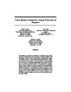
(2) as a result of “hard” splitting of input space. Each individual expert is trained individually on subsets of instances contained in these local regions, and finally the output of only one specialized expert is taken into consideration. Indeed, if the regions are non-intersecting then there is no reason to combine the outputs of different experts or modules and only one of them is explicitly used (a particular case when the weights of other experts are zero). In tree-like models such regions are constructed progressively narrowing the regions of the input space. The result is a hierarchy, a tree (often a binary one) with splitting rules in non-terminal nodes and the expert models in leaves (Fig. 1). Such models will be called in this paper mixtures of local experts (MLEs) and the experts will be referred to as modules, or specialized models. Models in MLEs could be of any type. If the model output is a nominal variable so that the classification problem is to be solved, then one of the popular methods is a decision tree. For solving numerical prediction (regression) problem, there is a number of methods that are based on the idea of a decision tree: (a) regression tree by Breiman et al. [4], where a leave is associated with an average output value of the instances sorted down to it (zero-order model), and (b) model tree, where leaves have regression functions of the input variables. In model trees, two approaches can be distinguished: one by Friedman [10] in the MARS (multiple adaptive regression splines) algorithm implemented as MARS software, and M5 model trees by Quinlan [20] implemented in Cubist software and, with some changes, in Weka software ([8]). The mentioned algorithms are suboptimal, “greedy”, since the choice of attribute for a split node is made once and is not reconsidered. The subject at this paper is optimisation of building LMEs consisting of simple (linear) regression models. M5 algorithm is chosen as the basic greedy algorithm allowing for building LMEs of linear models. Aim is to propose an approach allowing for building optimal LMEs. M5 algorithm is analogous to ID3 decision tree algorithm of Quinlan (also greedy) in a sense that it minimizes the intrasubset variation in the output values down each branch. In each node, the standard deviation of the output values for the examples reaching a node is taken as a measure of the error of this node and calculating the expected reduction in error as a result of testing each attribute and possible split values. Such

split attribute together with the split value that maximize the expected error reduction are chosen for each node. The splitting process will terminate if the output values of all the instances that reach the node vary only slightly or only a few instances remain. After the initial tree has been grown, the linear regression models are generated, and, possibly, simplified, pruned and smoothed. Wang & Witten [7] reported M5’ algorithm based on the original M5 algorithm but able to deal with enumerated attributes, to treat missing values and a different splitting termination condition.

Training Data Set

a1 New instance

a2

M3

a4

M1

a3

M4

where Mopt is a model with optimal configuration, {Mk} is a set of all possible model configurations, E is a model error. For the purpose of this paper it will be assumed that M is a LME and consists of a number of individual models Mi. In order to be more specific, we will limit the type of LME by assuming that a LMEs is built via a tree-like approach like M5. 2.2. Step-wise model construction The idea of optimisation is based on a simple empirical idea aimed at avoiding solving an overall hard optimization problem by splitting the generation of a LME into two steps: 1. Global optimisation. Generate upper layers of the tree (from the 1st layer) by a global (multi-extremum) optimization algorithm (better-than-greedy); 2. Greedy search. Generate the rest of the tree (lower layers) by a faster greedy algorithm like M5 [20], [32]. The layer up to which global optimization is applied could be different in different branches, as illustrated on Fig. 2. However, it would be reasonable to fix it at some value for all branches; in this case it will be denoted as L. This allows for a flexible trade-off between speed and optimality.

M5

a1 M2

Global Optimization

Output

a2

a4

Fig. 1: Consecutive application of rules in a tree-like structure leading to a local expert a1

2. Optimization of LMEs In the context of classification problems, a number of researchers aimed at improving the predictive accuracy of a tree-based model; they dealt mostly with decision trees and with greedy approaches: [5], [7], [9], [15], [19], and [23]. A rare exception of using a non-greedy approach for constructing decision trees was reported by Bennett [1]: the tree is represented as a system of linear inequalities and the system is solved using the iterative linear programming Frank-Wolfe method. The experiments indicated the advantages of the proposed method but also indicated that it may be trapped in a local minimum. To avoid that Bennett & Blue [2] used an Extreme Point Tabu Search (EPTS); it performed better than C4.5 on all 10 dataset tested. The problem of optimizing construction of local regression models like M5 tree is, however, addressed very little. 2.1. Optimization of LMEs The problem of building a LME can be posed in a general way ensuring that the error of the resulting overall model is minimal among all possible configurations: Find such Mopt that E(Mopt) = min, M ⊂ {Mk} ( 1 )

Greedy algorithm

a5

a3

a1

a1

a4

a5

a1

M8

a2

M3

a2

M9

M4

Fig. 2: Optimizing construction of a tree-like LME

2.3. M5opt algorithm for building LMEs The algorithmic approach presented above allows for the use of any type of the local regression model in the leaves of the generated tree. An implementation of this approach is the M5opt algorithm oriented at building the LMEs with linear regression models in the leaves, i.e. M5 model trees, and using exhaustive search is presented below. By a “tree structure” we understand an encoding of a tree which however does not have the associated split attributes and

2

values. By alg_parameters all the parameters specific to a particular implementation of M5 algorithm are understood. Input: instances, alg_parameters, number_of_attributes Output: Most_accurate_model_tree 1. Generate all trees structures {Ti} with the user defined tree layer 2. For each valid tree structure Ti do step 3-8 3. NOnes = the number of 1’s in the current tree Ti 4. Generate all possible attribute combinations corresponding to the tree nodes: Aj (NOnes, number_of_attributes) 5. For each attribute combination Aj do step 6-8 6. Build the current model tree based on Aj, alg_parameters 7. If the current model tree is more accurate than the Most_accurate_model_tree 8. then Replace the Most_accurate_model_tree with the current model tree 9. Stop.

2.4. Optimization of the upper subtree 1) Exhaustive search: The problem of overal tree optimization can be computationally costly since each attribute should be tested across a number of possible split values. The full problem of optimal binary decision tree construction (which is in essence applied in M5 as well) is reported to be NP-complete [13]. 2) M5opt with the randomized search: In order to find an estimate of the global optimum when the objective function is not known analytically, a number of methods could be applied. Random search techniques are most widely used for this purpose – genetic and evolutionary algorithms, controlled random search, adaptive cluster covering, tabu search, simulated annealing, and others ([16], [24], [29]). Evolutionary and genetic algorithms (GA) are among the popular techniques of global optimization, especially for discrete problems. A chromosome (or string) cab be encoded as integer-valued vectors representing a collection of attributes with the values in the range of [0, n] where n is the number of attributes. The position of particular element in the chromosome indicates the node position in the tree. The element value is the number of the attribute selected for this node; element zero means there is no node in the corresponding position of the tree. Chromosomes not corresponding to feasible trees are discarded. Software like GLOBE [11] allowing for using a number of global optimisation algorithms can be employed. The formulation of M5opt with GA as an optimizer for building M5 trees is similar to the version of the algorithm with exhaustive search presented above. 2.5. Additional features of M5opt M5 builds the initial model tree in a way similar to regression trees (Breiman et al., 1984) where each node is characterized by its split attribute and value, and by the averaged output values of the instances that reach a node. This latter is used for measuring the error of the initial model tree. M5opt algorithm, however, is able to build a linear model for the instances that reach a node, directly in the

initial model tree. This allows obtaining more accurate model already at initial stage. A better version of pruning (called compacting) was proposed as well.

3. Experiments For experiments we employed five benchmark data sets (Autompg, Bodyfat, CPU, Friedman and Housing) from Blake and Mertz [3], three hydrological data sets of Sieve catchment (Italy), and three hydrological data sets of Bagmati catchment (Nepal). The problem associated with hydrological data sets is to predict runoffs Qt+i several hours ahead (i=1, 3 or 6) on the basis of previous runoffs (Qt-τ) and effective rainfalls (REt-τ), τ being between 0 and 2. Before building a prediction model, it was necessary to analyze the physical characteristics of the catchment and then to select the input and output variables by analyzing the inter-dependencies between variables and the lags τ using correlation and average mutual information analysis. The final forms of the model of Sieve catchment are as follows: Qt+1 = f (REt, REt-1, REt-2, REt-3, REt-4, REt-5, Qt, Qt-1, Qt-2) Qt+3 = f (REt, REt-1, REt-2, REt-3, Qt, Qt-1) Qt+6 = f (REt, Qt,) The model for Bagmati case was set to be Qt+1 = f (REt, REt-1, REt-2, Qt, Qt-1) In Bagmati case study the data set was separated into high flows (>300 m3/s) and low flows, and two separate models were built. Three methods were employed: M5', M5opt and ANN (MLP). 1) M5’ models were built based on default parameter values of Weka software [32]: pruning factor 2.0 and employing smoothing. The same parameter settings were also used in M5opt experiments. 2) M5opt model trees allow for setting a large number of parameters’ combinations. In the experiments twelve various combinations were investigated; the best combinations reported here used the exhaustive search for subtrees of up to L=3 levels. More details on the parameters settings can be found in [22]. 3) ANNs were built using NeuroSolutions [17] and NeuralMachine software [18]. The best network appeared to be a three-layered perceptron (MLP) with 18 hidden nodes and hyperbolic tangent as activation functions. The stopping criteria was either mean squared error in training reaching the threshold of 0.0001 or the number of epochs reaching 5000.

4. Results and Discussion Algorithms' performance was measured by root mean squared error (RMSE) and the overall experimental results

3

TABLE 2 SCORING MATRIX FOR ALL ON ALL 11 VERIFICATION DATA SETS

are summarized in Table 1. M5opt model trees were the most accurate on seven data sets, and ANN on the other four. A so-called scoring matrix SM was used to present the results in a comparative way. This is a square matrix with the element SMi,j representing the average of relative performance of algorithm i compare to algorithm j with respect to all data sets used (diagonal elements are zero):

RMSE k , j − RMSE k ,i 1 , i≠ j  ∑ (2) SM i , j =  N k =1 max( RMSE k , j , RMSE k ,i ) 0, i = j  where N is the number of data sets. By summing up all the elements’ values column-wise one can determine the overall score of each algorithm, with the best algorithm having the highest positive score. M5opt has the highest score of 27.8. The experiments with M5opt indicated that the use of exhaustive search in building model trees could indeed give higher accuracy. Apart from the non-greedy optimization, an additional feature that was implemented in M5opt was improved pruning (compacting) scheme. The advantages of using it are: (1) the resulting model tree can be simpler (as simple as the user wants) and (2) the model tree itself is more balanced – this is desirable for the practical applications. To see the effect of optimization and compacting, compare model trees built for one of the case studies (Sieve Qt+6): M5’ tree has 7 rules with RMSE 22.894 (Fig. 3a), but M5opt has only 2 rules with RMSE 19.867 (Fig. 3b).

ANN

ANN 0

M5' 2.428

M5opt 13.871

M5'

-2.428

0

13.914

M5opt

-13.871

-13.914

0

Total

-16.299

-11.487

27.785

N

TABLE 1 RMSE OF M5’, M5OPT AND ANN ON ALL DATA SETS

Data sets

ANN Train. Verif.

Train.

M5' M5opt Verif. Train. Verif.

Sieve catchment 7.946 Qt+1 15.18 Qt+3 28.89 Qt+6

8.476 12.76 20.23

4.550 13.09 26.47

3.612 13.67 22.89

4.614 14.23 28.60

3.110 11.82 19.35

Bagmati catchment 97.34 All 224.6 High 31.92 Low

158.4 173.5 29.26

93.67 249.6 30.03

152.8 187.3 31.18

99.26 222.2 30.44

145.5 178.7 30.78

Benchmark data sets Auto-mpg 2.12 0.843 Body-fat 9.578 CPU Friedman 1.023

2.308 0.655 53.80 1.157

2.521 0.848 28.48 2.218

2.489 0.573 43.44 2.204

2.434 0.719 18.71 1.902

2.448 0.402 26.32 1.982

2.844

2.822

2.258

2.510

1.795

Housing

1.905

The superior performance of M5opt, even being tested on a limited number of examples, allows to assume that the approach used in the proposed framework may improve accuracy of other types of tree-like LMEs like CART and C4.5. More detailed analysis of the statistical properties of the proposed framework and the error margins of its performance are yet to be done.

5. Conclusion The proposed empirical algorithmic framework, combining greedy and non-greedy approaches to building local mixtures of experts, allows for flexible trade-off between speed and optimality. Its particular implementation, M5opt algorithm, makes it possible to construct modular linear regression models (M5 model trees) that are more accurate than the traditional greedy approach of M5 and M5’. The performance of M5opt with relation to ANN was investigated as well. The results indicate that M5opt outperforms M5’ on all cases and outperforms ANN on 8 out of 11 cases. An important advantage of regression and model trees in comparison with ANNs is their transparent structure providing a domain expert with a simple and reproducible data-driven model ([26]). Additional computational costs associated with a higher level of optimization (problem is NP-complete if fully exhaustive search is employed [13]) can be user-controlled by selecting the appropriate tree layer until which the non-greedy search is executed, and the type of search employed (exhaustive or randomised). Research is planned to apply the proposed approach to decision and regression trees, and to include non-linear regression models like MLPs and RBF networks to serve as local experts.

4

[6]

[7]

[8] [9]

[10] [11] a) Local expert models generated by M5 algorithm

[12] [13] [14] [15]

b) Local expert models generated by M5opt algorithm Fig. 3: Sieve Qt+6 cases study. Models generated by (a) M5’ and (b) M5opt algorithms. Numbers in parentheses given after liner models (LM) are numbers of examples sorted to this model and, after slash, RMSE divided by average absolute deviation, expressed in %. It can be seen that M5opt generates smaller and more accurate models.

[16]

References:

[17] [18]

[1]

[19]

[2] [3]

[4] [5]

Bennett, K.P., Global tree optimization: a non-greedy decision tree algorithm, Journal of Computing Science and Statistics, 26, 1994, 156-160. Bennett, K.P., & Blue, J.A., Optimal decision trees. R.P.I. Math Report No. 214., 1997. Blake, C.L., & Mertz, C.J., UCI Repository of machine learning databases. http://www.ics.uci.edu/ ~mlearn/MLRepository.html, Irvine, CA: University of California, Department of Information and Computer Science. Breiman, L., Friedman, J.H., Olshen, R.A., & Stone, C.J., Classification and regression trees (Wadsworth International, Belmont, CA., 1984). Caruana, R., & Freitag, D., Greedy attribute selection, Proc. International Conference on Machine Learning, 1994, 28-36.

[20]

[21] [22]

[23]

5

Drucker, H., Improving Regressor using Boosting. Proc. of the 14th Int. Conf. on Machine Learning, Douglas H. Fisher, Jr (Eds.), Morgan Kaufmann,1997, 107-115. Frank, E., & Witten, I.H., Selecting multiway splits in decision trees, Working paper 96/31, Dept. of Computer Science, University of Waikato, December, 1996. Frank, E., Wang, Y., Inglis, S., Holmes, G., & Witten, I.H., Using model trees for classification, Journal of Machine Learning, 32(1), 1998, 63-76. Freund, Y. & Mason, L. The alternating decision tree learning algorithm. Proc. 16th International Conf. on Machine Learning, Morgan Kaufmann, San Francisco, CA, 1999, 124-133. Friedman, J.H. Multivariate adaptive regression splines, Annals of Statistics, 19, 1991, 1-141. GLOBE: global and evolutionary optimisation tool, http://www.data-machine.com. Haykin, S. Neural networks. Second edition, PrenticeHall, 1999. Hyafil, L. & Rivest, R.L. Constructing Optimal Binary Decision Trees is NP-complete, Information Processing Letters, 5, 1976, 15-17. Jacobs, R.A., Jordan, M.I., Nowlan, S.J., & Hinton, G.E. Adaptive mixtures of local experts, Neural Computation, 3, 1991, 79-87. Kamber, M., Winstone, L., Gong, W., Cheng, S., & Han, J. Generalization and decision tree induction: efficient classification in data mining, Proc. of International workshop on research issues on data engineering (RIDE’97), Birmingham, England, April 1997, 111-20. Michalewicz, Z. Genetic algorithms + data structures = evolution programs. Third edition (Springer-Verlag, Hiedelberg, Germany, 1999). NeuroSolutions software. http://www.nd.com. NeuralMachine software: a neural network tool. http://www.data-machine.com. Pfahringer, B., Geoffrey, H., & Kirkby, R. Optimizing the induction of alternating decision trees, Proc. of the Fifth Pasific-Asia Conf. on Advances in Knowledge Discovery and Data Mining, 2001. Quinlan, J.R. Learning with continuous classes, Proc. AI’92, 5th Australian Joint Conference on Artificial Intelligence, Adams & Sterling (eds.), World Scientific, Singapore, 1992, 343-348. Quinlan, J.R., C4.5: Programs for Machine Learning, Morgan Kaufmann, San Mateo, CA, 1993. Siek, M.B.L.A., Flexibility and optimality in model tree learning with application to water-related problems, MSc Thesis Report, IHE Delft, Netherlands, 2003. Sikonja, M.R. & Kononenko, I., Pruning regression trees with MDL, ECAI 98, 13th European Conference on Artificial Intelligence, 1998.

[24]

[25]

[26]

[27]

Solomatine, D.P., Two strategies of adaptive cluster covering with descent and their comparison to other algorithms, Journal of Global Optimization, 14(1), 1999, 55-78. Solomatine, D.P., Applications of data-driven modelling and machine learning in control of water resources, Computational intelligence in control, M. Mohammadian, R.A. Sarker and X. Yao (eds.), Idea Group Publishing, 2002, 197 - 217. Solomatine, D.P., & Dulal, K.N., Model tree as an alternative to neural network in rainfall-runoff modelling, Hydrological Sciences Journal, 48(3), 2003, 399-411. Solomatine, D.P., Mixture of simple models vs ANNs in hydrological modelling, Proc. 3rd International Conference on Hybrid Intelligent Systems (HIS’03), Melbourne, December 2003.

[28]

[29] [30] [31]

[32]

6

D.P. Solomatine and D.L. Shrestha, AdaBoost.RT: a Boosting Algorithm for Regression Problems, Proc. 2004 Joint Conference on Neural Networks (IJCNN2004), Budapest, Hungary, 25-29 July 2004, 11631168. Törn, A. & Zilinskas, A., Global optimization, Springer-Verlag, Berlin, 1989, 255pp. Utgoff, P.E., Berkman, N.C., & Clouse, J.A., Decision tree induction based on efficient tree restructuring. Journal of Machine Learning, 29(1), 1997, 5-44. Wang, Y., & Witten, I.H., Induction of model trees for predicting continuous classes, Proc. of the European Conference on Machine Learning, Prague, Czech Republic, 1997, 128-137. Witten, I.H. and Frank, E., Data Mining, Morgan Kaufmann Publishers, 2000.