optimizing object-based classification in urban environments using ...

ISPRS Annals of the Photogrammetry, Remote Sensing and Spatial Information Sciences, Volume I-7, 2012 XXII ISPRS Congress, 25 August – 01 September 2012, Melbourne, Australia

OPTIMIZING OBJECT-BASED CLASSIFICATION IN URBAN ENVIRONMENTS USING VERY HIGH RESOLUTION GEOEYE-1 IMAGERY M.A. Aguilar a,*, R. Vicente a, F.J. Aguilar a, A. Fernández b, M.M. Saldaña a a

High School Engineering, Department of Agricultural Engineering, Almería University, 04120 La Cañada de San Urbano, Almería, Spain - [email protected], [email protected], [email protected], [email protected] b Escola de Enxeñaría Industrial, Department of Engineering Design, Vigo University, Campus Universitario, 36310 Vigo, Spain - [email protected] Commission VII, WG VII/4

KEY WORDS: Classification, Land Cover, Accuracy, Imagery, Pushbroom, High resolution, Satellite, Multispectral

ABSTRACT: The latest breed of very high resolution (VHR) commercial satellites opens new possibilities for cartographic and remote sensing applications. In fact, one of the most common applications of remote sensing images is the extraction of land cover information for digital image base maps by means of classification techniques. When VHR satellite images are used, an object-based classification strategy can potentially improve classification accuracy compared to pixel based classification. The aim of this work is to carry out an accuracy assessment test on the classification accuracy in urban environments using pansharpened and panchromatic GeoEye-1 orthoimages. In this work, the influence on object-based supervised classification accuracy is evaluated with regard to the sets of image object (IO) features used for classification of the land cover classes selected. For the classification phase the nearest neighbour classifier and the eCognition v. 8 software were used, using seven sets of IO features, including texture, geometry and the principal layer values features. The IOs were attained by eCognition using a multiresolution segmentation approach that is a bottom-up regionmerging technique starting with one-pixel. Four different sets or repetitions of training samples, always representing a 10% for each classes were extracted from IOs while the remaining objects were used for accuracy validation. A statistical test was carried out in order to strengthen the conclusions. An overall accuracy of 79.4% was attained with the panchromatic, red, blue, green and near infrared (NIR) bands from the panchromatic and pansharpened orthoimages, the brightness computed for the red, blue, green and infrared bands, the Maximum Difference, a mean of soil-adjusted vegetation index (SAVI), and, finally the normalized Digital Surface Model or Object Model (nDSM), computed from LiDAR data. For buildings classification, nDSM was the most important feature attaining producer and user accuracies of around 95%. On the other hand, for the class “vegetation”, SAVI was the most significant feature, obtaining accuracies close to 90%.

VHR is a very challenging task and has been the focus of intensive research for the last decade.

1. INTRODUCTION With the launch of the first very high resolution (VHR) satellites such as IKONOS in September 1999 or QuickBird in October 2001, conventional aerial photogrammetric mapping at large scales began to have serious competitors. In this way and in Spain there have already been several operational applications using QuickBird for othoimage generation covering large regions such as Murcia. In 2008 was launched a new commercial VHR satellite called GeoEye-1 (GeoEye, Inc.), which, nowadays, is the commercial satellite with the highest geometric resolution, in panchromatic (0.41 m) and in multispectral (1.65 m) products. More recently, on January 4, 2010, have begun to commercialize imagery of the last of the VHR satellites launched. It is WorldView-2 (DigitalGlobe, Inc.), whose more relevant technical innovation is the radiometric accuracy improvement, since the number of bands that compose its multispectral image are increased to 8, instead of the 4 classic bands (R, G, B, NIR) of all the previous VHR satellites.

The high resolution satellite images are being increasingly used for the detection of the buildings. Of the techniques used, automatic image classification is the most widely used technique for the detection of buildings. But very high resolution of the input image is usually joined to a high local variance of urban land cover classes. In this way, their statistical separability is limited using traditional pixel-based classification approaches. Thus, classification accuracy is reduced and the results could show a “salt and pepper” effect (e.g., Treitz and Howarth, 2000). Classification accuracy is particularly problematic in urban environments, which typically consist of mosaics of small features made up of materials with different physical properties (Mathieu et al., 2007). To overcome this problem, object-based classification can be used (Carleer and Wolff, 2006; Blaschke 2010). The aim of this work is to carry out an accuracy assessment test on the classification accuracy in urban environments using GeoEye-1 orthoimages. In this assay, the influence on supervised object-based classification accuracy is going to be evaluated with regard to the sets of image object (IO) features used for classification of the land cover classes selected. Concretely, seven sets of IO features are tested. A statistical test is carried out in order to strengthen the conclusions.

Many recent studies have used (VHR) satellite imagery for extracting georeferenced data in urban environments (e.g., Turker and San, 2010; Pu et al., 2011). In fact some of them used the newest GeoEye’s satellite for extracting buildings (e.g., Hussain et al., 2011; Grigillo and Kosmatin Fras, 2011). Concretely, automatic building extraction or classification from

*

Corresponding author

99

ISPRS Annals of the Photogrammetry, Remote Sensing and Spatial Information Sciences, Volume I-7, 2012 XXII ISPRS Congress, 25 August – 01 September 2012, Melbourne, Australia

Normalized Digital Surface Model (nDSM) was generated by subtracting DEM from DSM. In this way the buildings can be easily distinguished (Fig. 2). Also, orthoimages with 15 cm GSD were attained from this flight by Intergraph Z/I Imaging DMC (Digital Mapping Camera).

2. STUDY SITE AND DATASETS 2.1 Study site The study area comprises the little village of Villaricos, Almería, Southern Spain, including an area of 17 ha (Fig. 1). The working area is centered on the WGS84 coordinates (Easting and Northing) of 609,007 m and 4,123,230 m.

Figure 1. Location of the working area.

Figure 2. From left to right, details of pansharpened orthoimage, SAVI index, and nDSM.

2.2 GeoEye-1 orthoimages

3. METHODOLOGY

Over the study site an image of GeoEye-1 Geo from the imagery archive of GeoEye was acquired. It was captured in reverse scan mode on 29 September 2010, recording the panchromatic (PAN) band and all four multispectral (MS) bands (i.e., R, G, B and NIR). Finally, image products were resampled to 0.5 m and 2 m for the PAN and MS cases respectively. For these products, the pancharpened image with 0.5 m GSD and containing the four bands from MS image was attained using the PANSHARP module included in PCI Geomatica v. 10.3.2 (PCI Geomatics, Richmond Hill, Ontario, Canada). Finally, two orthoimages (PAN and pansharpened) were computed using the photogrammetric module of PCI Geomatica (OrthoEngine). Rational function model with a zero order transformation in image space, 7 DGPS ground control points and a very accurate LiDAR derived digital elevation models (which is going to be detailed later) were used for obtaining both orthoimages. These orthophotos presented a planimetric accuracy of 0.46 m, measured as root mean square error (RMSE) at 75 independent check points (Aguilar et al., 2012).

3.1 Multiresolution segmentation The object-based image analysis software used in this research was eCognition v. 8.0. This software uses a multiresolution segmentation approach that is a bottom-up region-merging technique starting with one-pixel objects. In numerous iterative steps, smaller IOs are merged into larger ones (Baatz and Schäpe, 2000). But this task is not easy, and it depends on the desired objects to be segmented (Tian and Chen, 2007).

2.3 Soil adjusted vegetation index (SAVI) Vinciková et al. (2010) reported that between the most commonly used vegetation indices in remote sensing applications are the Normalized Difference Vegetation Index (NDVI) and the Soil Adjusted Vegetation Index (SAVI). In fact, the attained results using these methods were very similar. In our work SAVI index was used. It was computed by SAVI algorithm from PCI Geomatica, and a new image was calculated from Red and NIR bands included in pansharpened orthoimage (Fig. 2).

Figure 3. Multiresolution segmentation. Left: Scale 20 at pixel level. Right: Scale 70 above. However, this work is not focused on VHR segmentation. So, and after visually inspecting the degree to which IOs matched the feature boundaries of the land cover types in the study area, we used the multiresolution segmentation with a scale of 20 at the first, and at the pixel level. Finally, a scale of 70 on the first segmentation level was used (Fig. 3). The segmentation was always developed using the four equal-weighed bands from pansharpened orthoimage. Furthermore, the compactness was assigned a weight of 0.5 and the shape was fixed at 0.3. Following this way, 2723 IOs were detected. For using this segmentation into ArcGis v. 9.3 and carrying out the following phases of manual classification and training areas selection,

2.4 Normalized Digital Surface Model (nDSM) The digital elevation model (DEM) and digital surface model (DSM) used in this work were a high accuracy and resolution LiDAR derived DEM with a grid spacing of 1 m. This LiDAR data was taken on August 28th, 2009, as a combined photogrammetric and LiDAR survey at a flying height above ground of approximately 1000 m. A Leica ALS60 airborne laser scanner (35 degree field of view, FOV) was used with the support of a nearby ground GPS reference station, being 1.61 points/m2 the average point density. The estimated vertical accuracy computed from 62 ICPs took a value of 8.9 cm. The

100

ISPRS Annals of the Photogrammetry, Remote Sensing and Spatial Information Sciences, Volume I-7, 2012 XXII ISPRS Congress, 25 August – 01 September 2012, Melbourne, Australia

neighbour classifier. For example, the 298 IOs from “Red Buildings” class had a mean area of 74.5 m2 per object, presenting a high standard deviation of 51.6 m2. Thus, for every different repetition chosen in this work, training areas for “Red Buildings” were always composed by 30 objects with a mean area of around 74 m2. The selection of training areas was developed into ArcGis, and after it was exported as GEOTIFF file. Four GEOTIFF files (four repetitions of training samples containing about 10% of total objects) were finally attained. They were imported into eCognition as a Test and Training Area mask (TTA Mask), and later on they were converted to samples for carrying out the training task.

2723 IOs were exported from eCognition as a shapefile vector data format (.SHP). 3.2 Manual Classification Only 1894 IOs from the initial 2723 could be visually indentified as meaningful objects. The hand-made or manual classification was developed into ArcGis v. 9.3 using the available datasets (orthoimages from GeoEye-1 and DMC, MDE, DSM, nDSM, SAVI). Table 1 shows the correctly manual classified IOs in each of the ten considered classes. A subset of 945 well-distributed IOs were selected to carry out the training phase of the classifier used in this work (i.e., nearest neighbour). The remaining 949 IOs, also well-distributed in the working area, were used for the validation or accuracy assessment phase. For each class, approximately a 50% of IOs were in the training subset, while the other 50% were selected for the validation subset. Subset IOs Subset IOs Validation Training Red buildings 298 149 149 White buildings 558 279 279 Grey buildings 68 34 34 Other buildings 55 28 27 Shadows 477 239 238 Vegetation 194 97 97 Bare soil 93 47 46 Roads 72 36 36 Streets 71 36 35 Swimming pools 8 4 4 Table 1. IOs after the segmentation process. Class

No. IOs

3.3 Training areas In this work, an object-based supervised classification has been used, being nearest neighbour the classifier chosen. In this type of automatic classification, the accuracy is a function of the training data used in its generation, principally size and quality (e.g., Foody and Mathur, 2006). Guidance on the design of the training phase of a classification typically calls for the use of a large sample of randomly selected pure or meaningful objects in order to characterise the classes.

Feature

Description

Blue Green Red NIR Pan SAVI Bright Max. Diff. nDSM NDBI Std. Blue Std. Green Std. Red Std. NIR Std. Pan Std. SAVI Ratio 1 Ratio 2 Ratio 3 Ratio 4 Ratio 5 Ratio 6 Hue

Mean of pansharpened GeoEye-1 blue band Mean of pansharpened GeoEye-1 green band Mean of pansharpened GeoEye-1 red band Mean of pansharp GeoEye-1 infrared band Mean of panchromatic GeoEye-1 band Mean of soil-adjusted vegetation index Average of means of four pansharp bands Maximum difference between bands Digital Surface Model or Object Model Normalized Difference of Blue band Index Standard deviation of blue Standard deviation of green Standard deviation of red Standard deviation of infrared Standard deviation of pan Standard deviation of SAVI Ratio to scene for blue band Ratio to scene for green band Ratio to scene for red band Ratio to scene for infrared band Ratio to scene for pan band Ratio to scene for SAVI band Mean of Hue image processed from pansharpened GeoEye-1 bands RGB Mean of Intensity image processed from pansharpened GeoEye-1 bands RGB Mean of Saturation image processed from pansharpened GeoEye-1 bands RGB The product of the length and the width of the corresponding object and divided by the number of its inner pixels. The border length of the IO divided by four times the square root of its area The ratio of the area of a polygon to the area of a circle with the same perimeter The number of edge that form the polygon GLCM homogeneity from infrared GLCM homogeneity from pan GLCM contrast from infrared GLCM contrast from pan GLCM dissimilarity from infrared GLCM dissimilarity from pan GLCM entropy from infrared GLCM entropy from pan GLCM standard deviation from infrared GLCM standard deviation from pan GLCM correlation from infrared GLCM correlation from pan GLDV angular second moment from infrared GLDV angular second moment from pan GLDV entropy from infrared GLDV entropy from pan GLDV contrast from infrared GLDV contrast from pan

Intensity Saturation Compact

Shape Index

2

Area of IOs (m ) No. Training IOs for each Standard Mean repetition Deviation 30 74 1.72 Red buildings 56 30 2.58 White buildings 7 77 3.37 Grey buildings 6 55 1.55 Other buildings 48 45 1.60 Shadows 20 89 1.64 Vegetation 10 166 2.74 Bare soil 8 218 5.24 Roads 8 103 2.99 Streets 1 43 9.36 Swimming pools Table 2. Characteristics of four IOs repetitions extracted for the classifier training.

Compactness

Class

Num. Edges GLCMH 1 GLCMH 2 GLCMC 1 GLCMC 2 GLCMD 1 GLCMD 2 GLCME 1 GLCME 2 GLCMStd 1 GLCMStd 2 GLCMCR 1 GLCMCR 2 GLDV2M 1 GLDV2M 2 GLDVE 1 GLDVE 2 GLDVC 1 GLDVC 2

In this work, four different repetitions of 10% IOs were extracted from the training subset of 945 IOs. This percentage was tried to keep constant for every classes, both in number of objects and in the mean area or size of them. In this way, Table 2 shows the number of IOs chosen for training the nearest

Table 3. Image Object (IO) features used in the classification phase.

101

ISPRS Annals of the Photogrammetry, Remote Sensing and Spatial Information Sciences, Volume I-7, 2012 XXII ISPRS Congress, 25 August – 01 September 2012, Melbourne, Australia

3.4

This accuracy assessment TTA Mask always included the same 949 IOs. Overall accuracy, producer’s accuracy and user’s accuracy were the studied values in this work. It is noteworthy that before computing these accuracy index, the four classes related with buildings (i.e., red, white, grey and other buildings) where grouped in only one class named buildings. Table 4 shows the area percentage occupied by the 1894 IOs which were manually classified. In the working area, “buildings” were the more extended class, following by “shadows”, “vegetation”, “bare soil” and “roads”. “Streets”, and especially “Swimming pools”, were the two classes with less area within the working area.

Feature extraction and selection

In addition to the four features (Red, Green, Blue and Infrared bands from pansharpened GeoEye-1 orthoimage) used for creating the IOs at the segmentation phase, other 43 features, described in Table 3, were used for supervised classification. A more in depth information about them could be found in the Definiens eCognition Developer 8 Reference Book (Definiens eCognition, 2009). The 47 features could be grouped as: (i) ten features were mean layer values, (ii) six standard deviation layer values, (iii) six ratios to scene layer values, (iv) three hue, saturation and intensity layer values, (v) two geometry features based on the shape, (vi) two geometry features based on polygons, and (vii) eighteen texture features based on the Haralick co-occurrence matrix (Haralick et al., 1973), as GrayLevel Co-occurrence Matrix (GLCM) or as Gray-Level Difference Vector (GLDV), always considering all the directions. A similar feature space for classification was utilized by previous researchers (Pu et al., 2011; Stumpf and Kerle, 2011).

3.6 Statistic analysis In order to study the influence of the studied factor (i.e., seven different strategies or features sets) on the final classification accuracy, an analysis of variance (ANOVA) test for one factor was carried out by means of a factorial model with four repetitions (Snedecor and Cochran, 1980). The observed variables were the overall accuracy, producer’s accuracy and user’s accuracy respectively. The source of variation was the set of features used for the nearest neighbour classifier. When the results of the ANOVA test turned out to be significant, the separation of means was carried out using the Duncan’s multiple range test at 95% confidence level.

Finally, seven sets of features were carried out for this work, and each of them supposed a different strategy for classification: (i) Set 1: This set is including only seven basic features of mean layer values such as Blue, Green, Red, Infrared, Pan, Brightness and Maximum difference. (ii) Set 2: It is composed by the seven basic features plus SAVI index. (iii) Set 3: It is formed by the seven basic features plus nDSM. (iv) Set 4: It is composed by the seven basic features plus SAVI and nDSM. (v) Set 5: Seven basic features plus SAVI and Normalized Difference of Blue band Index (NDBI), being the last computed as NDBI =(NIR−Blue)/(NIR+Blue). (vi) Set 6: Seven basic features plus CONTRAST texture feature (GLCM Contrast), computed from panchromatic band. (vii) Set 7: All the features presented in Table 3 except nDSM and NDBI.

4. RESULTS AND DISCUSSION Table 5 shows the overall accuracy results for each set of features tested in this work, considering the four classes related with buildings (i.e., red, white, grey and other buildings) grouped in one class named “buildings”. Sets 2 (7 basic features plus SAVI), 4 (7 basic features plus SAVI and nDSM), 5 (7 basic features plus SAVI and NDBI) and 7 (45 features) were the strategies with the best results. Although these four sets could not be statistically separated, globally and bearing in mind the extremely high computation time or “running time” needed for carried out the set 7 due to texture features principally, the best strategy could be the set 4, with nDSM and SAVI. Figure 4 shows a classification detail of one of the four repetitions using SAVI and nDSM, both for 10 classes and for 7 classes.

3.5 Classification and accuracy assessment

The following tables (5 to 10) try to assess the behaviour of the different sets of features or strategies tested in this work for the most relevant class. In all of them, values in the same column followed by different letters indicate significant differences at a significance level p < 0.05 and the bold values show the best significant accuracies.

For computing the classification, the seven sets of features were run applying standard nearest neighbour to classes. Bearing in mind that there were four repetitions of training samples, 28 different classification projects were carried out into eCognition. In all of them, the accuracy assessment was computed by mean of an error matrix based on a TTA Mask.

Features Overall Accuracy (%) Set 1 74.36 a Set 2 77.21 abc Set 3 75.92 ab Set 4 79.39 c Set 5 77.47 cb Set 6 75.66 ab Set 7 79.16 c Table 5. Comparison of mean values of Overall Accuracy for the seven set of features tested.

Occupied Grouped Occupied area (%) Class area (%) Red buildings 17.74 White buildings 13.60 Buildings 38.02 Grey buildings 4.22 Other buildings 2.46 Shadows 17.24 239 17.24 Vegetation 13.73 97 13.73 Bare soil 12.35 47 12.35 Roads 12.55 36 12.55 Streets 5.84 36 5.84 Swimming pools 0.27 4 0.27 Table 4. Area per class occupied by the 1894 IOs meaningful objects manual classified. Class

Regarding “buildings” class (Table 6), the most important feature for classifying them turned out to be the nDSM. This fact have already been reported by many authors such as Hermosilla et al. (2011), Awrangjeb et al. (2010), Turker and San (2010) or Longbotham et al. (2012). In our assay, both producer and user accuracy for buildings class were significantly better when nDSM was employed into the features

102

ISPRS Annals of the Photogrammetry, Remote Sensing and Spatial Information Sciences, Volume I-7, 2012 XXII ISPRS Congress, 25 August – 01 September 2012, Melbourne, Australia

set. In fact, a high accuracy level (around 95%) was reached using nDSM.

Shadows Producer’s Shadows User’s Features Accuracy (%) Accuracy (%) Set 1 87.99 87.87 Set 2 91.26 85.33 Set 3 85.38 85.03 Set 4 89.41 84.72 Set 5 90.89 85.22 Set 6 90.07 90.15 Set 7 92.46 91.23 Table 7. Comparison of mean values of producer’s and user’s accuracies for “shadows” class and the seven sets of features. Features

Vegetation Producer’s Vegetation User’s Accuracy (%) Accuracy (%) Set 1 74.02 a 84.62 bc Set 2 81.14 b 81.14 ab Set 3 70.02 a 72.97 a Set 4 79.10 ab 87.83 bc Set 5 83.04 ab 91.70 c Set 6 74.65 a 84.45 bc Set 7 88.43 b 86.36 bc Table 8. Comparison of mean values of producer and user accuracy for “vegetation” class and the seven set of features.

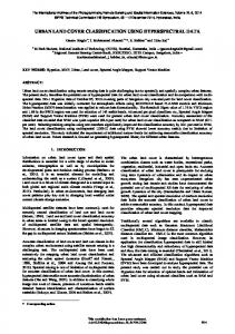
Figure 4. Classification detail of one of the four repetitions using SAVI and nDSM, with 10 classes (left above) and with 7 classes (left bellow). Class hierarchy is showed on the top right and samples for training are down to the right.

Features

Roads Producer’s Roads User’s Accuracy (%) Accuracy (%) Set 1 62.62 abc 61.88 Set 2 70.21 bc 62.77 Set 3 53.21 a 57.20 Set 4 59.00 abc 62.67 Set 5 72.21 c 63.39 Set 6 56.07 ab 59.54 Set 7 69.86 bc 68.16 Table 9. Comparison of mean values of producer’s and user’s accuracies for “Roads” class and the seven sets of features tested.

Regarding “shadows” class (Table 7), any features set was significantly better, although perhaps the texture feature “CONTRAST” could be highlighted. In the case of vegetation (Table 8), the best sets for producer accuracy were those which were containing the SAVI feature. With regard to user accuracy, both SAVI+nDSM (set 4) and SAVI+NDBI (set 5) were the best, although not significant features. For detecting vegetation, Zerbe and Liew (2004) pointed out that NDBI could help to distinguish vegetation class. In other way, authors as Haala and Brenner (1999) demonstrated the use of LiDAR to extract trees, besides buildings, in an urban area.

Features

Bare Soil Producer’s Bare Soil User’s Accuracy (%) Accuracy (%) Set 1 42.89 ab 44.30 ab Set 2 39.90 a 50.90 ab Set 3 41.59 a 44.52 ab Set 4 52.31 ab 49.57 ab Set 5 38.20 a 50.63 ab Set 6 57.84 b 49.96 ab Set 7 52.17 ab 53.77 b Table 10. Comparison of mean values of producer’s and user’s accuracies for “Bare Soil” class and the seven sets of features.

Regarding “roads” class (Table 9), nDSM and CONTRAST were the features with less repercussion in the classification results. On the other hand, using NDBI (set 5) the producer accuracy of the “roads” class was improved. Dinis et al. (2010) had already used this feature to discriminate between bare soil and roads in a QuickBird satellite image. “Bare soil” class had very poor results both in producer’s and user’s accuracies (Table 10). It could be due to the high heterogeneity of this class, which was including agricultural soils, non-asphalted road, building lots, and even beach.

5. CONCLUSION The accuracy assessment test on the supervised classification phase in urban environments using GeoEye-1 orthoimages, both pansharpened and panchromatic, and the statistical analysis carried out in this work has allowed us to draw the following conclusions:

Features

Buildings Producer’s Buildings User’s Accuracy (%) Accuracy (%) Set 1 88.90 a 83.05 a Set 2 90.27 ab 85.04 ab Set 3 94.98 c 95.46 c Set 4 95.18 c 95.35 c Set 5 90.51 ab 85.75 ab Set 6 89.26 a 86.50 ab Set 7 91.81 b 88.12 b Table 6. Comparison of mean values of producer’s and user’s accuracies for “buildings” class and the seven sets of features tested.

1.- Using seven basic features of mean layer values such as Blue, Green, Red, Infrared, Pan, Brightness and Maximum difference, a vegetation index as the Soil Adjusted Vegetation Index (SAVI), and the normalized Digital Surface Model or Object Model (nDSM), the best overall accuracy (79.39 %) was reached. This result improved even those carried out using 45 features, being the last strategy much more time consuming in terms of CPU.

103

ISPRS Annals of the Photogrammetry, Remote Sensing and Spatial Information Sciences, Volume I-7, 2012 XXII ISPRS Congress, 25 August – 01 September 2012, Melbourne, Australia

2.- nDSM was the most important feature for detecting buildings, as it had already reported by many authors working with other sources of images, such as Ikonos, WorldView-2, or digital aerial images. 3.- The inclusion of SAVI index was related with the detection of vegetation, and, together with NDBI, was a good strategy for the classification of roads. 4.- A percentage of 10% of training areas was enough for attaining good accuracies using object-based supervised classification with the nearest neighbour classifier.

Urban Remote Sensing Event --- Munich, Germany, April 1113, 2011. Haala, N. and Brenner, C., 1999. Extraction of buildings and trees in urban environments. ISPRS Journal of Photogrammetry and Remote Sensing, 54(2-3), pp. 130-137. Haralick, R.M., Shanmugam, K. and Dinstein, I., 1973. Textural features for image classification. IEEE Transactions on Geoscience and Remote Sensing, 3, pp. 610-621. Hermosilla, T., Ruiz, L.A., Recio, J.A. and Estornell, J., 2011. Evaluation of Automatic Building Detection Approaches Combining High Resolution Images and LiDAR Data. Remote Sensing, 3(2011), pp. 1188-1210.

6. ACKNOWLEDGEMENTS This work was supported by the Spanish Ministry for Science and Innovation (Spanish Government) and the European Union (FEDER founds) under Grant Reference CTM2010-16573. The authors also appreciate the support from Andalusia Regional Government, Spain, through the Excellence Research Project RNM-3575. Website of the CTM2010-16573 project: http://www.ual.es/Proyectos/GEOEYE1WV2/index.htm

Hussain, E., Ural, S., Kim, K., Fu, C., Shan, J., 2011. Building Extraction and Rubble Mapping for City Port-au-Prince Post2010 Earthquake with GeoEye-1 Imagery and Lidar Data. Photogrammetric Engineering and Remote Sensing, 77(10), pp. 1011-1023. Longbotham, N., Chaapel, C., Bleiler, L., Padwick, C., Emery, W.J. and Pacifici, F., 2012. Very High Resolution Multiangle Urban Classification Analysis. IEEE Transactions on Geoscience and Remote Sensing, 50(4), pp. 1155-1170.

7. REFERENCES Aguilar, M.A., Aguilar, F.J., Saldaña, M.M. and Fernández, I., 2012. Geopositioning accuracy assessment of GeoEye-1 Panchromatic and Multispectral imagery. Photogrammetric Engineering and Remote Sensing, 78(3), pp. 247-257.

Mathieu, R., J. Aryal, and Chong, A.K., 2007. Object-based classification of Ikonos imagery for mapping large-scale vegetation communities in urban areas. Sensors, 7(11), pp. 2860-2880.

Awrangjeb, M., Ravanbakhsh, M. And Fraser, C.S., 2010. Automatic detection of residential buildings using LIDAR data and multispectral imagery. ISPRS Journal of Photogrammetry and Remote Sensing, 65(2010), pp. 457-467.

Pu, R., Landry, S. and Yu, Q., 2011. Object-based urban detailed land cover classification with high spatial resolution IKONOS imagery. International Journal of Remote Sensing, 32(12), pp. 3285-3308.

Baatz, M. and Schäpe, M., 2000. Multiresolution segmentation An optimization approach for high quality multi-scale image segmentation. In: Strobl, J., Blaschke, T., Griesebner, G. (Eds.), Angewandte Geographische Informations-Verarbeitung XII. Wichmann Verlag, Karlsruhe, pp. 12-23.

Snedecor, G.W. and Cochran, W.G., 1980. Statistical Methods. Seventh edition. Iowa State University Press, Ames, Iowa. 507 pages. Stumpf, A. and Kerle, N., 2011. Object-oriented mapping of landslides using Random Forests. Remote Sensing of Environment, 115(2011), pp. 2564-2577.

Blaschke, T., 2010. Object based image analysis for remote sensing. ISPRS Journal of Photogrammetry and Remote Sensing, 65(2010), pp. 2-16.

Tian, J. and Chen, D.M., 2007. Optimization in multi-scale segmentation of high-resolution satellite images for artificial feature recognition. International Journal of Remote Sensing, 28(20), pp. 4625-4644.

Carleer, A.P. and Wolff, E., 2006. Region-based classification potential for land-cover classification with very high spatial resolution satellite data. In: Proceedings of 1st International Conference on Object-based Image Analysis (OBIA 2006), Salzburg University, Austria, July 4-5, 2006. Vol. XXXVI.

Treitz, P. And Howarth, P.J., 2000. High spatial resolution remote sensing data for forest ecosystem classification: An examination of spatial scale, Remote Sensing of Environment, 72, pp. 268-289.

Definiens eCognition, 2009. Definiens eCognition Developer 8 Reference Book. Definiens AG, München, Germany. Dinis, J., Navarro A., Soares, F., Santos, T., Freire, S., Fonseca, A., Afonso, N., Tenedório, J., 2010. Hierarchical object-based classification of dense urban areas by integrating high spatial resolution satellite images and LiDAR elevation data. The International Archives of the Photogrammetry, Remote Sensing and Spatial Information Sciences, Vol. XXXVIII-4/C7.

Turker, M. and San, K., 2010. Building detection from pansharpened Ikonos imagery through support vector machines classification. The International Archives of the Photogrammetry, Remote Sensing and Spatial Information Science, Vol. XXXVIII, Part 8, Kyoto Japan 2010. Vinciková, H., Hais, M., Brom, J., Procházka, J. and Pecharová, E., 2010. Use of remote sensing methods in studying agricultural landscapes - a review. Journal of Landscape Studies, 3(2010), pp. 53-63.

Foody, G.M. and Mathur, A., 2006. The use of small training sets containing mixed pixels for accurate hard image classification: Training on mixed spectral responses for classification by a SVM. Remote Sensing of Environment, 103(2006), pp. 179-189.

Zerbe, L.M. and Liew, S.C., 2004. Reevaluating the traditional maximum NDVI compositing methodology: The Normalized Difference Blue Index. In: Geoscience and Remote Sensing Symposium, 2004. IGARSS '04. Proceedings. 2004 IEEE International, vol.4, pp. 2401-2404.

Grigillo, D. and Kosmatin Fras, M., 2011. Classification Based Building Detection From GeoEye-1 Images. In: Stilla U, Gamba P, Juergens C, Maktav D (Eds) JURSE 2011 - Joint

104