Different application development tools have not been well integrated or automated. The methodology to improve software performance, i.e. performance tuning ...
OPTIMIZING PARALLEL APPLICATIONS
by Shih-Hao Hung
A dissertation submitted in partial fulfillment of the requirements for the degree of Doctor of Philosophy (Computer Science and Engineering) in The University of Michigan 1998
Doctoral Committee: Professor Edward S. Davidson, Chair Professor William R. Martin Professor Trevor N. Mudge Professor Quentin F. Stout
©Shih-Hao Hung
All Rights Reserved
1998
For my family.
ii
ACKNOWLEDGMENT I owe a special thanks to my advisor, Professor Edward S. Davidson. Without his support, guidance, wisdom, and kindly revising my writing, my study toward Ph.D degree and writing this dissertation would have been much more painful. I would like to thank Prof. Gregory Hulbert, Prof. William Martin, Prof. Trevor Mudge, and Prof. Quentin Stout for their advises that helped improve this dissertation. I would like to thank Ford Motor Company, Automative Research Ceter (U.S. ArmyTACOM), and the National Partnership for Advanced Computational Infrastructure (NPACI, NSF Grant No. ACI-961920) for their generous financial support of this research. Parallel computer time was provided by the University of Michigan Center of Parallel Computing which is sponsored in part by NSF grant CDA-92-14296. Thanks to CPC staff, particularly Paul McClay, Andrew Caird, and Hal Marshall, for providing excellent technical support on the KSR, HP/Convex Exemplar, IBM SP2, and SGI PowerChallenger. I have been fortunate to meet numerous marvelous fellow students in the Parallel Performance Project (formerly the Ford Project). Lots of my work in this dissertation has been inspired or based on their research. These are what I learned from these friends who have been my officemates in 2214 EECS: hierarchical performance bounds models (Tien-Pao Shih, Eric Boyd), synthetic workload (Eric Boyd), domain decomposition (Karen Tomko), relaxed synchronization (Alex Eichenberger), and machine performance evaluation (Gheith Abandah). Thanks to Ed Tam and Viji Srinivasan for letting me use their cache simulation tools. Jude Rivers has been a bright, delightful fellow of mine, whose constant skeptical attitude toward parallel computing has been one motivation for this research. Thanks to many people, Ann Arbor has been a very wonderful place to me in the last 5 years. To people who I have played volleyball, basketball, softball, and majong with. To people who lend me tons of anime to kill countless hours. To my family back in Taiwan for their full support of my academic career over the years. To our cute little black cat, Ji-Ji, for bringing lots of laughters to our home. Finally, to my lovely wife, Weng-Ling, for always finding ways to make our lives here more interesting and meaningful. iii
TABLE OF CONTENTS DEDICATION .................................................................................... ii ACKNOWLEDGMENT ....................................................................... iii LIST OF TABLES ............................................................................ vii LIST OF FIGURES ......................................................................... viii CHAPTER 1 INTRODUCTION ...................................................................................... 1 1.1
Parallel Machines .................................................................................... 3 1.1.1 Shared-Memory Architecture - HP/Convex Exemplar ............... 4 1.1.2 Message-Passing Architecture - IBM SP2 .................................. 5 1.1.3 Usage of the Exemplar and SP2.................................................. 6
1.2
Parallelization of Applications ................................................................ 7
1.3
Problems in Developing Irregular Applications ..................................... 9 1.3.1 Irregular Applications.................................................................. 9 1.3.2 Example - CRASH...................................................................... 10 1.3.3 Parallelization of CRASH .......................................................... 13 1.3.4 Performance Problems ............................................................... 14
1.4
Developing High Performance Parallel Applications........................... 15 1.4.1 Conventional Scheme................................................................. 16 1.4.2 Recent Trends............................................................................. 17 1.4.3 Problems in Using Parallel Tools .............................................. 18 1.4.4 The Parallel Performance Project ............................................. 19 1.4.5 Goals of this Dissertation .......................................................... 21
1.5
Summary and Organization of this Dissertation ................................. 22
2 ASSESSING THE DELIVERED PERFORMANCE .................................... 24 2.1
Machine Performance Characterization ............................................... 25
2.2
Machine-Application Interactions......................................................... 29 2.2.1 Processor Performance............................................................... 29 2.2.2 Interprocessor Communications................................................ 32 2.2.3 Load Balancing, Scheduling, and Synchronization.................. 33 iv
2.2.4 2.2.5
Performance Problems in CRASH-SP....................................... 35 Overall Performance .................................................................. 37
2.3
Performance Assessment Techniques................................................... 38 2.3.1 Source Code Analysis ................................................................. 38 2.3.2 Profile-Driven Analysis.............................................................. 39 2.3.3 Trace-driven Analysis ................................................................ 48 2.3.4 Other Approaches....................................................................... 51
2.4
Efficient Trace-Driven Techniques for Assessing the Communication Performance of Shared-Memory Applications...................................... 52 2.4.1 Overview of the KSR1/2 Cache-Only Memory Architecture .... 52 2.4.2 Categorizing Cache Misses in Distributed Shared-Memory Systems....................................... 55 2.4.3 Trace Generation: K-Trace ........................................................ 57 2.4.4 Local Cache Simulation: K-LCache........................................... 62 2.4.5 Analyzing Communication Performance with the Tools.......... 67
2.5
Summary ................................................................................................ 70
3 A UNIFIED PERFORMANCE TUNING METHODOLOGY ....................... 72 3.1
Step-by-step Approach ........................................................................... 73
3.2
Partitioning the Problem (Step 1) ......................................................... 74 3.2.1 Implementing a Domain Decomposition Scheme ..................... 75 3.2.2 Overdecomposition ..................................................................... 78
3.3
Tuning the Communication Performance (Step 2)............................... 79 3.3.1 Communication Overhead ......................................................... 79 3.3.2 Reducing the Communication traffic ........................................ 79 3.3.3 Reducing the Average Communication Latency ...................... 89 3.3.4 Avoiding Network Contention ................................................... 93 3.3.5 Summary .................................................................................... 95
3.4
Optimizing Processor Performance (Step 3)......................................... 96
3.5
Balancing the Load for Single Phases (Step 4) .................................. 100
3.6
Reducing the Synchronization/Scheduling Overhead (Step 5).......... 101
3.7
Balancing the Combined Load for Multiple Phases (Step 6)............. 105
3.8
Balancing Dynamic Load (Step 7)....................................................... 106
3.9
Conclusion ............................................................................................ 110
4 HIERARCHICAL PERFORMANCE BOUNDS AND GOAL-DIRECTED PERFORMANCE TUNING .................................................................... 116 4.1
Introduction.......................................................................................... 117 4.1.1 The MACS Bounds Hierarchy ................................................. 117 4.1.2 The MACS12*B Bounds Hierarchy......................................... 119 4.1.3 Performance Gaps and Goal-Directed Tuning........................ 120 v
4.2
Goal-Directed Tuning for Parallel Applications................................. 120 4.2.1 A New Performance Bounds Hierarchy .................................. 120 4.2.2 Goal-Directed Performance Tuning ........................................ 123 4.2.3 Practical Concerns in Bounds Generation .............................. 124
4.3
Generating the Parallel Bounds Hierarchy: CXbound ...................... 125 4.3.1 Acquiring the I (MACS$) Bound ............................................. 125 4.3.2 Acquiring the IP Bound ........................................................... 126 4.3.3 Acquiring the IPC Bound......................................................... 127 4.3.4 Acquiring the IPCO Bound ...................................................... 128 4.3.5 Acquiring the IPCOL Bound ................................................... 129 4.3.6 Acquiring the IPCOLM Bound ................................................ 129 4.3.7 Actual Run Time and Dynamic Behavior ............................... 131
4.4
Characterizing Applications Using the Parallel Bounds ................... 133 4.4.1 Case Study 1: Matrix Multiplication....................................... 133 4.4.2 Case Study 2: A Finite-Element Application.......................... 140
4.5
Summary .............................................................................................. 143
5 MODEL-DRIVEN PERFORMANCE TUNING ........................................ 147 5.1
Introduction.......................................................................................... 147
5.2
Application Modeling ........................................................................... 151 5.2.1 The Data Layout Module ......................................................... 154 5.2.2 The Control Flow Module ........................................................ 155 5.2.3 The Data Dependence Module................................................. 168 5.2.4 The Domain Decomposition Module ....................................... 170 5.2.5 The Weight Distribution Module............................................. 173 5.2.6 Summary of Application Modeling .......................................... 174
5.3
Model-Driven Performance Analysis .................................................. 175 5.3.1 Machine Models........................................................................ 176 5.3.2 The Model-Driven Simulator................................................... 176 5.3.3 Current Limitations of MDS ................................................... 178
5.4
A Preliminary Case Study ................................................................... 180 5.4.1 Modeling CRASH-Serial, CRASH-SP, and CRASH-SD......... 181 5.4.2 Analyzing the Performance of CRASH-Serial, CRASH-SP, and CRASH-SD ........................................................................ 185 5.4.3 Model-Driven Performance Tuning......................................... 194 5.4.4 Summary of the Case Study .................................................... 216
5.5
Summary .............................................................................................. 216
6 CONCLUSION ...................................................................................... 219
REFERENCES ................................................................................ 222
vi
LIST OF TABLES Table 1-1 2-1 2-2 2-3 2-4 2-5 2-6 2-7 3-1 3-2 4-1 5-1 5-2 5-3 5-4 5-5 5-6 5-7 5-8 5-9 5-10 5-11 5-12 5-13 5-14 5-15
Vehicle Models for CRASH............................................................................. 13 Some Performance Specifications for HP/Convex SPP-1000........................ 26 The Memory Configuration for HP/Convex SPP-1000 at UM-CPC ............. 26 Microbenchmarking Results for the Local Memory Performance on HP/Convex SPP-1000 ................................................................................ 27 Microbenchmarking Results for the Shared-Memory Point-to-Point Communication Performance on HP/Convex SPP-1000 ...... 27 Collectable Performance Metrics with CXpa, for SPP-1600......................... 42 D-OPT Model for characterizing a Distributed Cache System. ................... 56 Tracing Directives........................................................................................... 62 Comparison of Dynamic Load Balancing Techniques ................................ 109 Performance Tuning Steps, Issues, Actions and the Effects of Actions. (1 of 2)...................................................................... 114 Performance Tuning Actions and Their Related Performance Gaps. (1 of 2) ................................................... 145 A Run Time Profile for CRASH.................................................................... 182 Computation Time Reported by MDS.......................................................... 186 Communication Time Reported by MDS. .................................................... 186 Barrier Synchronization Time Reported by MDS ....................................... 186 Wall Clock Time Reported by MDS. ............................................................ 186 Hierarchical Parallel Performance Bounds (as reported by MDS) and Actual Runtime (Measured).................................................................. 188 Performance Gaps (as reported by MDS). ................................................... 188 Working Set Analysis Reported by MDS..................................................... 188 Performance Metrics Reported by CXpa (Only the Main Program Is Instrumented). ................................................ 191 Wall Clock Time Reported by CXpa............................................................. 191 CPU Time Reported by CXpa....................................................................... 191 Cache Miss Latency Reported by CXpa....................................................... 191 Cache Miss Latency and Wall Clock Time for a Zero-Workload CRASH-SP, Reported by CXpa........................................ 192 Working Set Analysis Reported by MDS for CRASH-SP, CRASH-SD, and CRASH-SD2........................................................................................... 199 PSAT of Arrays Position, Velocity, and Force in CRASH........................... 207
vii
LIST OF FIGURES Figure 1-1 1-2 1-3 1-4 1-5 2-1 2-2 2-3 2-4 2-5 2-6 2-7 2-8 2-9 2-10 2-11 2-12 3-1 3-2 3-3 3-4 3-5 3-6 3-7 3-8 3-9 3-10 3-11 3-12 3-13 3-14 4-1
HP/Convex Exemplar System Overview. ........................................................ 4 Example Irregular Application, CRASH. ...................................................... 11 Collision between the Finite-Element Mesh and an Invisible Barrier. ....... 12 CRASH with Simple Parallelization (CRASH-SP). ...................................... 15 Typical Performance Tuning for Parallel Applications. ............................... 16 Performance Assessment Tools...................................................................... 25 Dependencies between Contact and Update ................................................. 36 CPU Time of MG, Visualized with CXpa....................................................... 43 Workload Included in CPU Time and Wall Clock Time. .............................. 45 Wall Clock Time Reported by the CXpa. ....................................................... 46 Examples of Trace-Driven Simulation Schemes. .......................................... 50 KSR1/2 ALLCache. ......................................................................................... 53 An Example Inline Tracing Code. .................................................................. 59 A Parallel Trace Consisting of Three Local Traces....................................... 60 Trace Generation with K-Trace. .................................................................... 61 Communications in a Sample Trace. ............................................................. 64 Coherence Misses and Communication Patterns in an Ocean Simulation Code on the KSR2................................................... 69 Performance Tuning. ...................................................................................... 72 An Ordered Performance-tuning Methodology ............................................. 73 Domain Decomposition, Connectivity Graph, and Communication Dependency Graph .............................................................. 76 A Shared-memory Parallel CRASH (CRASH-SD) ........................................ 76 A Message-passing Parallel CRASH (CRASH-MD), A Psuedo Code for First Phase is shown. ...................................................... 78 Using Private Copies to Enhance Locality and Reduce False-Sharing ....... 84 Using Gathering Buffers to Improve the Efficiency of Communications .... 85 Communication Patterns of the Ocean Code with Write-Update Protocol. 87 Communication Patterns of the Ocean Code with Noncoherent Loads....... 87 Example Pairwise Point-to-point Communication........................................ 93 Communication Patterns in a Privatized Shared-Memory Code ................. 94 Barrier, CDG-directed Synchronization, and the Use of Overdecomposition............................................................... 103 Overdecomposition and Dependency Table................................................. 103 Approximating the Dynamic Load in Stages. ............................................ 108 Performance Constraints and the Performance Bounds Hierarchy. ......... 121 viii
4-2 4-3 4-4 4-5 4-6 4-7 4-8 4-9 4-10 4-11 4-12 4-13 4-14 4-15 4-16 5-1 5-2 5-3 5-4 5-5 5-6 5-7 5-8 5-9 5-10 5-11 5-12 5-13 5-14 5-15 5-16 5-17 5-18 5-19 5-20 5-21 5-22 5-23 5-24 5-25
Performance Tuning Steps and Performance Gaps. ................................... 123 Calculation of the IPCO, IPCOL, IPCOLM, IPCOLMD Bounds. .............. 130 An Example with Dynamic Load Imbalance. .............................................. 132 The Source Code for MM1. ........................................................................... 134 Parallel Performance Bounds for MM1. ...................................................... 135 Performance Gaps for MM1. ........................................................................ 135 The Source Code for MM2. ........................................................................... 136 Parallel Performance Bounds for MM2. ...................................................... 136 Comparison of MM1 and MM2 for 8-processor Configuration. .................. 137 Source Code for MM_LU .............................................................................. 138 Performance Bounds for MM_LU ................................................................ 139 Performance Comparison of MM2 on Dedicated and Multitasking Systems .......................................................... 139 Performance Bounds for the Ported Code.................................................... 140 Performance Bounds for the Tuned Code.................................................... 142 Performance Comparison between Ported and Tuned on 16-processor Configuration ..................................................................... 142 Model-Driven Performance Tuning. ............................................................ 149 Model-driven Performance Tuning. ............................................................. 151 Building an Application Model..................................................................... 152 An Example Data Layout Module for CRASH. ........................................... 154 A Control Flow Graph for CRASH. .............................................................. 157 The Tasks Defined for CRASH..................................................................... 158 A Hierarchical Control Flow Graph for CRASH. ........................................ 159 An IF-THEN-ELSE Statement Represented in a CFG. ............................. 159 A Control Flow Module for CRASH. ............................................................ 160 Program Constructs and Tasks Modeled for CRASH ................................. 162 A Control Flow Graph for a 2-Processor Parallel Execution in CRASH-SP. ............................................................................................... 163 Associating Tasks with Other Modules for Modeling CRASH-SP on 4 Processors. ........................................................ 164 Modeling the Synchronization for CRASH-SP. ........................................... 166 Modeling the Point-to-Point Synchronization, an Example. ...................... 167 A Data Dependence Module for CRASH. .................................................... 169 An Example Domain Decomposition Module for CRASH-SP. ................... 171 Domain Decomposition Schemes Supported in MDS. ................................ 172 An Example Domain Decomposition for CRASH-SD. ................................ 172 An Example Workload Module for CRASH/CRASH-SP/CRASH-SD......... 173 Model-driven Analyses Performed in MDS. ................................................ 175 An Example Machine Description of HP/Convex SPP-1000 for MDS. ................................................................... 176 A Sample Input for CRASH. ........................................................................ 180 Decomposition Scheme Used in CRASH-Serial, SP, and SD. .................... 184 Performance Bounds and Gaps Calculated for CRASH-Serial, CRASH-SP, and CRASH-SD.............................................. 187 The Layout of Array Position in the Processor Cache in CRASH-SD........ 190
ix
5-26 Comparing the Wall Clock Time Reported by MDS and CXpa. ............................................................................................ 194 5-27 Performance Bounds Analysis for CRASH-SP. ........................................... 195 5-28 Performance Bounds Analysis for CRASH-SP and SD............................... 196 5-29 Layout of the Position Array in the Processor Cache in CRASH-SD2....... 197 5-30 Comparing the Performance Gaps of CRASH-SD2 to Its Predecessors. ... 198 5-31 Comparing the Performance of CRASH-SD2 to Its Predecessors.............. 199 5-32 A Pseudo Code for CRASH-SD3................................................................... 200 5-33 Comparing the Performance Gaps of CRASH-SD3 to Its Predecessors. ... 201 5-34 Comparing the Performance of CRASH-SD3 to Its Predecessors.............. 202 5-35 A Pseudo Code for CRASH-SD4................................................................... 203 5-36 Comparing the Performance of CRASH-SD4 to Its Predecessors.............. 204 5-37 The Layout in CRASH-SD2, SD3, SD4, SD5, and SD6. ............................. 205 5-38 Comparing the Performance of CRASH-SD5 to CRASH-SD4. .................. 206 5-39 Comparing the Performance of CRASH-SD6 to Previous Versions........... 208 5-40 Delaying Write-After-Read Data Dependencies By Using Buffers............ 209 5-41 The Results of Delaying Write-After-Read Data Dependencies By Using Buffers........................................................................................... 210 5-42 A Pseudo Code for CRASH-SD7................................................................... 211 5-43 Performance Bounds Analysis for CRASH-SD5, SD6, and SD7. ............... 212 5-44 A Pseudo Code for CRASH-SD8................................................................... 214 5-45 Data Accesses and Interprocessor Data Dependencies in CRASH-SD8.... 215 5-46 Performance Bounds Analysis for CRASH-SD6, SD7, and SD8. ............... 215 5-47 Summary of the Performance of Various CRASH Versions. ...................... 217 5-48 Performance Gaps of Various CRASH Versions. ........................................ 217
x
CHAPTER 1. INTRODUCTION “A parallel computer is a set of processors that are able to work cooperatively to solve a computational problem” [1]. Today, various types of parallel computers serve different usages ranging from embedded digital signal processing to supercomputing. In this dissertation, we focus on the application of parallel computing to solve large computational problems fast. Highly parallel supercomputers, with up to thousands of microprocessors, have been developed to solve problems that are beyond the reach of any traditional single processor supercomputer. By connecting multiple processors to a shared memory bus, parallel servers/ workstations have emerged as a cost-effective alternative to mainframe computers. While parallel computing offers an attractive perspective for the future of computers, the parallelization of applications and the performance of parallel applications have limited the success of parallel computing. First, applications need to be parallel or parallelized to take advantage of parallel machines. Writing parallel applications or parallelizing existing serial applications can be a difficult task. Second, parallel applications are expected to deliver high performance. However, more often than not, the parallel execution overhead results in unexpectedly poor performance. Compared to uniprocessor systems, there are many more factors that can greatly impact the performance of a parallel machine. It is often a difficult and timeconsuming process for users to exploit the performance capacity of a parallel computer, which generally requires them to deal with limited inherent parallelism in their applications, inefficient parallel algorithms, overhead of parallel execution, and/or poor utilization of machine resources. The latter two problems are what we intend to address in this dissertation. Parallelization is a state-of-the-art process that has not yet been automated in general. Most programmers have been trained in and have experience with serial codes and there exist many important serial application codes that could well benefit from the performance increases offered by parallel computers. Automatic parallelization is possible for loops where data dependency can be analyzed by the compiler. Unfortunately, the complexity of interpro-
1
cedural data flow analysis often limits automatic parallelization to basic loops without procedure calls. Problems can occur even in these basic loops if, for example, there exist indirect data references such as pointers or indirectly-indexed arrays. Fortunately, many of those problems are solvable with some human effort, especially from the programmers themselves, to assist the compiler. Regardless of whether parallelization is automatic or manual, high performance parallel applications are needed to better serve the user community. So far, while some parallel applications do successfully achieve high delivered performance, many others only achieve a small fraction of peak machine performance. It is often beyond the compiler’s or the application developer’s ability to accurately identify and consider the many machine-application interactions that can potentially affect the performance of the parallelized code. Over the last several decades, during which parallel computer architectures have constantly been modified and improved, tuned application codes and software environments for these architectures have had to be discontinued and rebuilt. Different application development tools have not been well integrated or automated. The methodology to improve software performance, i.e. performance tuning, like parallelization, has never been mature enough to reduce the tuning effort to routine work that can be performed by compilers or average programmers. Poor performance and painful experiences in performance tuning have greatly reduced the interest of many programmers in parallel computing. These problems must be solved to permit routine development of high performance parallel applications. Irregular applications [2] (Section 1.3), including sparse problems and those with unstructured meshes, often require more human parallel programming effort than regular applications, due to their indirectly indexed data items and irregular load distribution among the problem subdomains. Most full scale scientific and engineering applications exhibit such irregularity, and as a result they are more difficult to parallelize, load balance and optimize. Due to the lack of systematic and effective performance-tuning schemes, many irregular applications exhibit deficient performance on parallel computers. In this dissertation, we aim to provide a unified approach to addressing this problem by integrating performance models, performance-tuning methodologies and performance analysis tools to guide the parallelization and optimization of irregular applications. This approach will also apply to the simpler problem of parallelizing and tuning regular applications.
2
In this chapter, we introduce several key issues in developing high performance applications on parallel computers. Section 1.1 classifies parallel architectures and parallel programming models and describes the parallel computers that we use in our experiments. Section 1.2 describes the process and some of the difficulties encountered in the parallelization of applications. In Section 1.3, we discuss some aspects of irregular applications and the performance problems they pose. In Section 1.4, we give an overview of current application development environments and define the goals of our research. Section 1.5 summarizes this chapter and overviews the organization of this dissertation.
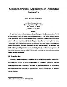
1.1 Parallel Machines There are various kinds of parallel computers, as categorized by Flynn [3]. We focus on multiple instruction stream, multiple data stream (MIMD) machines. MIMD machines can be further divided into two classes: shared-memory and message-passing. These two classes of machines differ in the type and amount of hardware support they provide for interprocessor communication. Interprocessor communications are achieved via different mechanisms on shared-memory machines and message-passing machines. A shared-memory architecture provides a globally shared physical address space, and processors can communicate with one another by sharing data with commonly known addresses, i.e. global variables. There may also be local or private memory spaces that belong to one processor or cluster of processors and are protected from being accessed by others. In distributed shared-memory (DSM) machines, logically shared memories are physically distributed across the system, and nonuniform memory access (NUMA) time results as a function of the distance between the requesting processor and the physical memory location that is accessed. In a message-passing architecture, processors have their own (disjoint) memory spaces and can therefore communicate only by passing messages among the processors. A message-passing architecture is also referred to as a distributed-memory or a shared-nothing architecture. In this section, we briefly discuss two cases that represent current design trends in shared-memory architectures (the HP/Convex Exemplar) and message-passing architectures (the IBM SP2). The Center for Parallel Computing of the University of Michigan (CPC) provides us with access to these machines.
3
1.1.1 Shared-Memory Architecture - HP/Convex Exemplar The HP/Convex1 Exemplar SPP-1000 shared memory parallel computer was the first model in the Exemplar series. It has 1 to 16 hypernodes, with 4 or 8 processors per hypernode, for a total of 4 to 128 processors. Processors in different hypernodes communicate via four CTI (Coherent Toroidal Interconnect) rings. Each CTI ring supports global memory accesses with the IEEE SCI (Scalable Coherent Interface) standard [4]. Each hypernode on the ring is connected to the next by a pair of unidirectional links. Each link has a peak transfer rate of 600MB/sec. Within each hypernode, four functional blocks and an I/O interface communicate via a 5port crossbar interconnect. Each functional block contains two Hewlett-Packard PARISC7100 processors [5] running at 100MHz, 2 banks of memory and controllers. Each processor has a 1MB instruction cache and a 1MB data cache on chip. Each processor cache is a
Functional Block M M
P
F.B.
F.B.
F.B.
hypernode 0
P
C I/O Interface 5-port crossbar
Functional Block M M
P
F.B.
F.B.
F.B.
hypernode n
P
C I/O Interface 5-port crossbar
F.B. - Functional Block P - Processor M - Memory C - Controllers
CTI rings
Figure 1-1: HP/Convex Exemplar System Overview.
1. Convex Computer Company was acquired by Hewlett-Packard (HP) in 1996. As of 1998, Convex is a division of HP and is responsible for the service and future development of the Exemplar series.
4
direct-mapped cache with a 32-byte line size. Each hypernode contains 256MB to 2GB of physical memory, which is partitioned into three sections: hypernode-local, global, and CTIcache. The hypernode-local memory can be accessed only by the processors within the same hypernode as the memory. The global memory can be accessed by processors in any hypernode. The CTIcaches reduce traffic on the CTI rings by caching global data that was recently obtained by this hypernode from remote memory (i.e. memory in some other hypernode). The eight physical memories in each hypernode are 8-way interleaved by 64-byte blocks. The basic transfer unit on the CTI ring is also a 64-byte block. The CPC at the University of Michigan was among the first sites with a 32-processor SPP1000 as the Exemplar series was introduced in 1994. In August, 1996, the CPC upgraded the machine to an SPP-1600. The primary upgrade in the SPP-1600 is the use of more advanced HP PA-RISC 7200 processors [6], which offer several major advantages over the predecessor, PA-RISC 7100: (1) Faster clock rate (the PA7200 runs at 120MHz), (2) the Runway Bus - a split transaction bus capable of 768 MB/s bandwidth, (3) an additional on-chip 2-KByte fullyassociative assist data cache, and (4) a four state cache coherence protocol for the data cache. The newest model in the Exemplar series is the SPP-2000, which incorporates HP PARISC 8000 processors [7]. The SPP-2000 has some dramatic changes in the architectural design of the processor and interconnection network, which provide a substantial performance improvement over the SPP-1600. Using HP PA-RISC family processors, the Exemplar series runs a version of UNIX, called SPP-UX, which is based on the HP-UX that runs on HP PARISC-based workstations. Thus, the Exemplar series not only maintains software compatibility within its family, but can also run sequential applications that are developed for HP workstations. In addition, using mass-produced processors reduces the cost of machine development, and enables more rapid upgrades (with minor machine re-design or modification), as new processor models become available.
1.1.2 Message-Passing Architecture - IBM SP2 The IBM Scalable POWERparallel SP2 connects 2 to 512 RISC System/6000 POWER2 processors via a communication subsystem, called the High Performance Switch (HPS). Each processor has its private memory space that cannot be accessed by other processors. The HPS is a bidirectional multistage interconnect with wormhole routing. The IBM SP2 at CPC has 64
5
nodes in four towers. Each tower has 16 POWER2 processor nodes. Each of the 16 nodes in the first tower has a 66 MHz processor and 256MB of RAM. Each node in the second and third towers has a 66 MHz processor and 128MB of RAM. The last 16 nodes each have a 160 MHz processor and 1GB of RAM. Each node has a 64KB data cache and 32 KB instruction cache. The line size is 64 bytes for the data caches and 128 bytes for the instruction caches. The SP2 runs the AIX operating system, a version of UNIX, and has C, C++, Fortran77, Fortran90, and High Performance Fortran compilers. Each POWER2 processor is capable of performing 4 floating-point operations per clock cycle. This system thus offers an aggregate peak performance of 22.9 GFLOPS. However, the fact that the nodes in this system differ in processor speed and memory capacity results in a heterogeneous system which poses additional difficulties in developing high performance applications. Heterogeneous systems, which often exist in the form of a network of workstations, commonly result due to incremental machine purchases. As opposed to heterogeneous systems, a homogeneous system, such as the HP/Convex SPP-1600 at CPC, uses identical processors and nodes, and this is easier to program and load-balance for scalability. In this dissertation, we focus our discussion on homogeneous systems, but some of our techniques can be applied to heterogeneous systems as well.
1.1.3 Usage of the Exemplar and SP2 The HP/Convex Exemplar and IBM SP2 at the CPC have been used extensively for developing and running production applications, as well as in performance evaluation research. Generally, shared-memory machines provide simpler programming models than messagepassing machines, as discussed in the next section. The interconnect of the Exemplar is focused more on reducing communication latency, so as to provide faster short shared-memory communications. The SP2 interconnect is focused more on high communication bandwidth, in order to reduce the communication time for long messages, as well as to reduce network contention. Further details of the Convex SPP series machines can be found in [8][9]. The performance of shared memory and communication on the SPP-1000 is described in detail in [10][11][12]. A comprehensive comparison between the SPP-1000 and the SPP-2000 can be found in [13]. Detailed performance characterizations of the IBM SP2 can be found in [14][15][16].
6
1.2 Parallelization of Applications Parallelism is the essence of parallel computing, and parallelization exposes the parallelism in the code to the machine. While some algorithms (i.e. parallel algorithms) are specially designed for parallel execution, many existing applications still use conventional (mostly sequential) algorithms and parallelization of such applications can be laborious. For certain applications, the lack of parallelism may be due to the nature of the algorithm used in the code. Rewriting the code with a parallel algorithm could be the only solution. For other applications, limited parallelism is often due to (1) insufficient parallelization by the compiler and the programmer, and/or (2) poor runtime load balance. In any case, the way a code is parallelized is highly related to its performance. To solve a problem by exploiting parallel execution, the problem must be decomposed. Both the computation and data associated with the problem need to be divided among the processors. As the alternative to functional decomposition, which first decomposes the computation, domain decomposition first partitions the data domain into disjoint subdomains, and then works out what computation is associated with each subdomain of data (usually by employing the “owner updates” rule). Domain decomposition is the method more commonly method used by programmers to partition a problem, because it results in a simpler programming style with a parallelization scheme that provides straightforward scaling to different numbers of processors and data set sizes. In conjunction with the use of domain decomposition, many programs are parallelized in the Single-Program-Multiple-Data (SPMD) programming style. In a SPMD program, one copy of the code is replicated and executed by every processor, and each processor operates on its own data subdomain, which is often accessed in globally shared memory by using index expressions that are functions of its Processor IDentification (PID). A SPMD program is symmetrical if every processor performs the same function on an equal-sized data subdomain. A near-symmetrical SPMD program performs computation symmetrically, except that one processor (often called the master processor) may be responsible for extra work such as executing serial regions or coordinating parallel execution. An asymmetrical SPMD program is considered as a Multiple-Programs-Multiple-Data (MPMD) program whose programs are packed into one code.
7
In this dissertation, we consider symmetrical or near-symmetrical SPMD programs that employ domain decomposition, because they are sufficient to cover a wide range of applications. Symmetrical or near-symmetrical SPMD programming style is favored not only because it is simpler for programmers to use, but also because of its scalability for running on different numbers of processors. Usually, a SPMD program takes the machine configuration as an input and then decomposes the data set (or chooses a pre-decomposed data set if the domain decomposition algorithm is not integrated into the program) based on the number of processors, and possibly also the network topology. For scientific applications that operate iteratively on the same data domain, the data set can often be partitioned once at the beginning and those subdomains simply reused in later iterations. For such applications, the runtime overhead for performing domain decomposition is generally negligible. Parallel programming models refer to the type of support available for interprocessor communication. In a shared-memory programming model, the programmers declare variables as private or global, where processors share the access to global variables. In a message-passing programming model, the programmers explicitly specify communication using calls to message-passing routines. Shared-memory machines support shared-memory programming models as their native mode; while block moves between shared memory buffer areas can be used to emulate communication channels for supporting message-passing programming models [8]. Message-passing machines can support shared-memory programming models via software-emulation of shared virtual memory [17][18]. Judiciously mixing shared-memory and message-passing programming models in a program can often result in better performance. The HP/Convex Exemplar supports shared-memory programming with automatic parallelization and parallel directives in its enhanced versions of C and Fortran. Message-passing libraries, PVM and MPI, are also supported on this machine. The SP2 supports Fortran 90 and High-Performance Fortran (HPF) [19] parallel programming languages, as well as the MPI [20], PVM [21], and MPL message-passing libraries. Generally, parallelization with sharedmemory models is less difficult than with message-passing models, because the programmers (or the compilers) are not required to embed explicit communication commands in the codes. Direct compilation of serial programs for parallel execution does exist today [22][23][24], but the state-of-the-art solutions are totally inadequate. Current parallelizing compilers have some success parallelizing loops where data dependency can be found . Unfortunately, prob-
8
lems often occur when there exist indirect data references or function calls within the loops, which causes the compiler to make safe, conservative assumptions, which in turn can severely degrade the attainable parallelism and hence performance and scalability. This problem limits the use of automatic parallelization in practice. Therefore, most production parallelizing compilers, e.g. KSR Fortran [25] and Convex Fortran [26][27], are of very limited use for parallelizing application codes. Interestingly, many of those problems can be solved by trained human experts. Use of conventional languages enhanced with parallel extensions, such as Message-Passing Interface (MPI), are commonly used by programmers to parallelize codes manually, and in fact many manually-parallelized codes perform better than their automatically-parallelized versions. So far, parallel programmers have been directly responsible for most parallelization work, and hence, the quality of parallelization today usually depends on the programmer’s skill. Parallelizing large application codes can be very time-consuming, taking months or even years of trial-and-error development, and frequently, parallelized applications need further fine tuning to exploit each new machine effectively by maximizing the application performance in light of the particular strengths and weakness of the new machine. Unfortunately, fine tuning a parallel application, even when code development and maintenance budgets would allow it, is usually beyond the capability of today’s compilers and most programmers. It often requires an intimate knowledge of the machine, the application, and, most importantly, the machine-application interactions. Irregular applications are especially difficult for the programer or the compiler to parallelize and optimize. Irregular application and their parallelization and performance problems are discussed in the next section.
1.3 Problems in Developing Irregular Applications 1.3.1 Irregular Applications Irregular applications are characterized by indirect array indices, sparse matrix operations, nonuniform computation requirements across the data domain, and/or unstructured problem domains [2]. Compared to regular applications, irregular applications are more difficult to parallelize, load balance and optimize. Optimal partitioning of irregular applications is an NP-complete problem. Compiler optimizations, such as cache blocking, loop transforma-
9
tions, and parallel loop detection, cannot be applied to irregular applications since the indirect array references are not known until runtime and the compilers therefore assume worst-case dependence. Interprocessor communications and the load balance are difficult to analyze without performance measurement and analysis tools. For many regular applications, domain decomposition is straightforward for programmers or compilers to apply. For irregular applications, decomposition of unstructured domains is frequently posed as a graph partitioning problem in which the data domain of the application is used to generate a graph where computation is required for each data item (vertex of the graph) and communication dependence between data items are represented by the edges. The vertices and edges can be weighted to represent the amount of computation and communication, respectively, for cases where the load is nonuniform. Weighted graph partitioning is an NP-complete problem, but several efficient heuristic algorithms are available. In our research, we have used the Chaco [28] and Metis [29] domain decomposition tools, which implement several algorithms. Some of our work on domain decomposition is motivated and/or based on profile-driven and multi-weight weighted domain decomposition algorithms developed previously by our research group [2][30].
1.3.2 Example - CRASH In this dissertation, an example application, CRASH, is a highly simplified code that realistically represents several problems that arise in an actual vehicle crash simulation. It is used here for demonstrating these problems and their solutions. A simplified high level sketch of the serial version of this code is given in Figure 1-2. CRASH exhibits irregularity in several aspects: indirect array indexing, unstructured meshes, and nonuniform load distribution. Because of its large data set size, communication overhead, multiple phase and dynamic load balance problems, this application requires extensive performance-tuning to perform efficiently on a parallel computer. CRASH simulates the collision of objects and carries out the simulation cycle by cycle in discrete time. The vehicle is represented by a finite element mesh which is provided as input to the code, such as illustrated in Figure 1-3. Instead of a mesh, the barrier is implicitly modeled as a boundary condition. Elements in the finite-element mesh are numbered from 1 to
10
program CRASH integer Type(Max_Elements),Num_Neighbors(Max_Elements) integer Neighbor(Max_Neighbors_per_Element,Max_Elements) real_vector Force(Max_Elements),Position(Max_Elements), Velocity(Max_Elements) real t, t_step integer i,j,type_element call Initialization c Main Simulation Loop t=0 c First phase: generate contact forces 100 do i=1,Num_Elements Force(i)=Contact_force(Position(i),Velocity(i)) do j=1,Num_Neighbors(i) Force(i)=Force(i)+Propagate_force(Position(i),Velocity(i), Position(Neighbor(j,i),Velocity(Neighbor(j,i)) end do end do c Second phase: update position and velocity 200 do i=1,Num_Elements type_element=Type(i) if (type_element .eq. plastic) then call Update_plastic(i, Position(i), Velocity(i), Force(i)) else if (type_element .eq. glass) then call Update_elastic(i, Position(i), Velocity(i), Force(i)) end if end do if (end_condition) stop t=t+t_step goto 100 end Figure 1-2: Example Irregular Application, CRASH. Num_Elements. Depending on the detail level of the vehicle model, the number of elements varies. Variable Num_Neighbors(i) stores the number of elements that element i interacts with (which in practice would vary from iteration to iteration). Array Neighbors(*,i) points to the elements that are connected to element i in the irregular mesh as well as other elements with which element i has come into contact during the crash. Type(i) specifies the type of material of element i. Force(i) stores the force calculated during contact that will be applied to element i. Position(i) and Velocity(i) store the position and velocity of element i. Force, position, and velocity of an element are declared as type real_vector variables, each of which is actually formed by three double precision (8-byte) floating-point numbers representing a three dimensional vector. Assuming the integers are 32-bits (4-bytes) 11
Time=Before Collision
Time=During Collision
Time=After Collision
Figure 1-3: Collision between the Finite-Element Mesh and an Invisible Barrier.
12
Vehicle Model
Num_Elements
Max_Neighbors_ per_Element
Working Set (Mbytes)
Small
10000
5
1
Large
100000
10
12
Table 1-1: Vehicle Models for CRASH. each, the storage requirement, or the total data working set, for CRASH is about (84+4*Max_Neighbor_per_Element)*Num_Elements bytes. In this dissertation, we assume two different vehicle models; their properties are shown in Table 1-1. The program calculates the forces between elements and updates the status of each element for each cycle. In the first phase, the Contact phase, the force applied to each element is calculated by calling Contact_force() to obtain and sum the forces between this element and other elements with which it has come into contact. In second phase, the Update phase, the position and velocity of each element are updated using the force generated in the contact phase. Depending on the type of material, the Update phase calls Update_Plastic() or Update_Elastic() for updating the position and velocity as a function of Force(i). Each cycle thus outputs a new finite-element mesh which is used as input to the next cycle. This example program shows irregularities in several aspects. First, objects are represented by unstructured meshes. Second, in the Contact phase, properties of neighbor elements are referenced with indirect array references, e.g. Velocity(Neighbor(j,i)), referring to the velocity of the j-th neighbor of element i. Third, the load is nonuniform because the load of calculating the force for an element during the Contact phase depends on how many neighbors each element has, and the load of updating the status of an element during the Update phase depends on the type of element being updated.
1.3.3 Parallelization of CRASH Even for codes as simple as CRASH, most parallelizing compilers fail to exploit the parallelism in CRASH because of the complexity of analyzing indirect array references, such as Velocity(Neighbor(j,i)), and procedure calls. The communication pattern needs to be explicitly specified for a message-passing version, yet determining the pattern is not a trivial
13
task. Fortunately, a shared-memory parallelization does not require the specification of an explicit communication pattern, and hence is initially much easier to develop. Performance tuning does, however, require some understanding of the communication pattern, in both cases. The parallelism in CRASH can quite easily be recognized by a parallel programmer: the calculations for different elements within each phase can be performed in parallel, because they have no data dependence. Manual parallelization of CRASH can be implemented by parallelizing the major loop in each phase (indexed by i). A straightforward, simple parallel version of CRASH on HP/Convex Exemplar, CRASH-SP, is illustrated in Figure 1-4. Note that the parallel directive, c$dir loop_parallel, is inserted ahead of each parallel loop. By default, loop_parallel instructs the compiler to parallelize the loop by partitioning the index into p subdomains: elements {1,2, ... N/p } are assigned to processor 1, elements { N/p+1 ... 2N/p } are assigned to processor 2, etc., where N is Num_Elements and p is the number of processors used in the execution. Since this parallelization partitions the domain into subdomains of nearly equal size, the workload will be evenly shared among the processors, if the load is evenly distributed over the index domain. However, for irregular applications like CRASH, this simple decomposition could lead to enormous communication traffic and poor load balance due to the unstructured meshes and nonuniform load distribution. More sophisticated domain decomposition algorithms are commonly used for partitioning the unstructured meshes so that the communication traffic is reduced [30].
1.3.4 Performance Problems In this dissertation, we focus on solving major performance problems resulting from irregular applications because they pose more difficult optimization problems and lack an effective general method to guide the programmers toward achieving high performance. Once such methods exist, regular applications may be handled as a degenerate case. These problems are described in the next chapter and are addressed throughout this dissertation.
14
program CRASH-SP integer Type(Num_Elements),Num_Neighbors(Num_Elements) integer Neighbor(Max_Neighbor_per_Elements,Num_Elements) real_vector Force(Num_Elements),Position(Num_Elements), Velocity(Num_Elements) real t, t_step integer i,j,Num_Neighbors,type_element call Initialization c Main Simulation Loop t=0 c First phase: generate contact forces c$dir loop_parallel 100 do i=1,Num_Elements Force(i)=Contact_force(Position(i),Velocity(i)) do j=1,Num_Neighbors(i) Force(i)=Force(i)+Propagate_force(Position(i),Velocity(i), Position(Neighbor(j,i),Velocity(Neighbor(j,i)) end do end do c Second phase: update position and velocity c$dir loop_parallel 200 do i=1,Num_Elements type_element=Type(i) if (type_element .eq. plastic) then call Update_plastic(i, Position(i), Velocity(i), Force(i)) else if (type_element .eq. glass) then call Update_glass(i, Position(i), Velocity(i), Force(i)) end if end do if (end_condition) stop t=t+t_step goto 100 end Figure 1-4: CRASH with Simple Parallelization (CRASH-SP).
1.4 Developing High Performance Parallel Applications Often, performance tuning is called hand tuning, which emphasizes the programer’s central role in most performance tuning work. While many people hope that someday compiler technology will automate most performance tuning work, most parallel programmers today are directly responsible for a large portion of the performance tuning work, which often requires extensive knowledge of the underlying hardware characteristics. Parallel programmers seem to spend more time poring over performance information and repeatedly modifying the source code in a cut-and-try approach, rather than simply deciding how best to tune the performance, and then simply doing it in one pass. In this section, we discuss this conven-
15
programmer
application
performance tools
machine
compiler
Figure 1-5: Typical Performance Tuning for Parallel Applications.
tional scheme, recent trends, current problems, and our approach for developing high performance applications.
1.4.1 Conventional Scheme Figure 1-5 shows how performance tuning is typically done today. The compiler transforms the source code into an executable code with optimizations derived from source-code analysis and programmer written directives. Although, theoretically, compilers could accept feedback from the execution and use it when deciding whether and how to apply certain optimizations, such as during instruction scheduling [31][32], no effective feedback mechanism exists today in any compiler that provides a sufficient amount of information to guide its optimizations. Performance enhancement is the programmer’s responsibility to carry out, primarily by revising the source code and modifying directives, perhaps with some help from performance assessment tools. The hardware details of a computer are usually hidden from the user by commonly used programming models. Programmers may ignore many hardware issues that can greatly degrade a code’s performance, even when substantial effort is spent varying the directives and flag settings for an optimizing compiler. As a result, hand tuning is subsequently involved to improve code performance, inefficient performance is accepted, or the parallel execution is 16
abandoned altogether. Under this conventional scheme, the effort to tune a parallel application, especially an irregular application, can be very time-consuming and/or ineffective. However, without proper tuning, peak performance on parallel computers, or even a respectable fraction of peak, can be very difficult to achieve. It should be no surprise that few tools can be used to facilitate the tuning, because for a long time, development of tools has been neglected or discontinued due to the typically short life times of parallel machines. Poor performance and painful experiences in performance tuning have greatly reduced the interest of many programmers in parallel computing. These are the major problems in a conventional parallel application development environment.
1.4.2 Recent Trends Until the early ‘90s, some optimistic researchers believed that parallelization could and would soon be fully automated and fairly well optimized by future parallelizing compilers, and some believed that parallel machines would then be able to carry out parallel execution fairly efficiently with a minimum of hand tuning. Unfortunately, parallelization and performance tuning turned out to be more difficult than they thought, and none of those expectations have been satisfied. More and more researchers realize that (1) manual parallelization is necessary and should be properly supported, and (2) the key to develop high performance applications lies in a strong understanding of the interactions between the machine and the application, i.e. machine-application interactions. Given these awareness, the parallel computing community started several projects (e.g. the Parallel Tools Consortium, est. 11/93) to promote the development of standardized application environments and performance tools to ease programmer’s burden and study machine-application interactions. Since then, more research has been focused on improving parallel tools, such as the following, to form a better application development environment:
• Standard Parallel Languages or Message-Passing Libraries, such as HPF [19] and MPI [20], which enable programmers to develop machine-independent codes and encourage vendors to optimize their machines for these languages. Among these new standards, MPI has been widely supported on almost all message-passing machines and even most sharedmemory machines (e.g. HP/Convex Exemplar).
17
• Parallelized and Tuned Libraries, such as Convex LAPACK [33], which ease the programmers’ burden by parallelizing and fine-tuning commonly-used routines. Many scientific/ engineering applications can benefit from the availability of such libraries.
• Domain Decomposition Packages, such as Chaco [28] and Metis [29], which provide various algorithms for decomposing irregular problem domains. With such packages, programmers are likely to save a considerable amount of time that would otherwise be spent writing and maintaining their own domain decomposition routines for irregular applications.
• Source-code Analyzers or Visualizers, such as APR Forge [34], which assist the users in parallelizing existing applications by revealing the data dependencies or data flow in the codes. Such tools directly assist the users, instead of attempting to accomplish automatic parallelization with a parallelizing compiler.
• Performance Assessment Tools, such as CXpa [35] and IBM PV [36], which assist the users in exploring the machine-application interactions in their applications. Performance assessment tools can be further categorized into three groups: performance extraction/ measurement, performance evaluation/characterization, and performance visualization. Performance extraction/measurement tools focus on finding specific events in the application and measuring their impact on the performance. Performance evaluation/characterization tools analyze the application performance, characterize the performance, and roughly identify the performance problems. Performance visualization tools provide a friendly graphics interface to help the users access and understand performance information. Note that some of these parallel tools address the problems in parallelizing applications, while some others, also known as performance tools, address the problems which limit the application performance. Often, these two goals are both considered by one tool, since the way that the code is parallelized is highly correlated with the application performance.
1.4.3 Problems in Using Parallel Tools Recent development of parallel tools has considerably improved the application development environment. However, current application development environments are still far from satisfactory. Typical problems that we have experienced are described below:
18
1. Lack of Tools and Difficulty of Using the Tools: While many tools have resulted from academic research, machine vendors have not been aggressively developing performance tools. According to the Ptools Consortium (http://www.ptools.org/): “Current parallel tools do not respond to the specific needs of scientific users who must become quasi-computer scientists to understand and use the tools”. 2. Lack of Tool Integration: Combining the use of different tools can be painful and tricky. For example, feeding performance information from the CXpa to Metis requires a mechanism to convert the performance data output from CXpa to a form that is accepted as input to Metis. Due to the lack of integration, programmers still need to spend a substantial amount of time in interfacing the use of tools. Such routine work should be automated as much as possible, allowing the programmers simply to monitor the process and make high-level decisions. 3. Unpredictable and Unreliable Tuning Methodologies: Programmers have been relying for better or worse on their personal experiences and trial-and-error processes in their practice of performance tuning. The learning curve is tedious and time consuming with no guarantee of how much if any performance improvement to expect for a particular application. Furthermore, because the side-effects of one optimization applied to solve one problem can expose or aggravate other problems, there are many cases where performance problems cannot be solved individually. 4. Unsuitable for Dynamic Applications: For one application, performance tuning may need to be repeated for different input data sets and different machines. Although integrating the performance tuning mechanism into the runtime environment would ameliorate this problem, runtime performance tuning is difficult to implement because performance tuning is far from automatic. Most performance tuning tools, either cannot be, or are not integrated into the runtime environment.
1.4.4 The Parallel Performance Project The Parallel Performance Project (PPP) research group was established at the University of Michigan (http://www.eecs.umich.edu/PPP/PPP.html) in 1992. The objective of our work is to develop and implement automated means of assessing the potential performance of applications on targeted supercomputers, high performance workstations and parallel computer systems, identifying the causes of degradations in delivered performance, and restructuring the application codes and their data structures so that they can achieve their full 19
performance potential. Many of the techniques presented in this dissertation are based on or motivated by some previous or concurrent work in the PPP group, including:
• Experiences in Hand-tuning Applications: We have worked jointly with scientists and engineers in developing high performance applications in various fields, including: (1) vehicle crash simulation with the Ford Motor Company, (2) ocean simulation for the Office of Naval Research, (3) modeling and simulation of ground vehicle with the Automotive Research Center (http://arc.engin.umich.edu/) for the U.S. Army (TACOM), and are continuing work of this kind on (4) antenna design and scattering analysis with the Radiation Laboratory at U. of Michigan (http://www.eecs.umich.edu/RADLAB/), (5) modeling soil vapor extraction and bioventing of organic chemicals in unsaturated geological material with the Environmental and Water Resources Engineering program at U. of Michigan (http://www-personal.engin.umich.edu/~abriola/simulation.html) for the U.S. Environmental Protection Agency, and (6) computer simulation of manufacturing processes of materials and structures with the Computational Mechanics Laboratory (http://www-personal.engin.umich.edu/~kikuchi/) at U. of Michigan. This ongoing work is supported in part by the National Partnership for Advanced Computational Infrastructure (NPACI) (http://www.npaci.edu/) of the National Science Foundation.
• Machine Performance Evaluation: The PPP group has developed performance evaluation methodologies (e.g. [37]) and tools (e.g. [38]) and has evaluated targeted high performance workstations (IBM RS/6000 [39][40], HP PA-RISC, DEC Alpha) and parallel computer systems (KSR1/2 [41][42], IBM SP2 [14][15], HP/Convex Exemplar [11][12][13], Cray T3D). The knowledge gained regarding target machines helps develop future machines and machine-specific performance tuning techniques [43].
• Goal-Directed Performance Tuning: A machine-application hierarchical performance bounds methodology has been developed to characterize the runtime overhead and guide optimizations (e.g. [44][45][46][47][48][49]). Major optimization techniques developed in the PPP group include data layout (e.g. [45][50]), restructuring data access patterns (e.g. [51]), communication latency hiding (e.g. [52]), instruction scheduling (e.g. [53][54]), and register allocation (e.g. [55][56]).
• Domain Decomposition Techniques and Advanced Synchronization Algorithms: Our experiences show that irregular problem domains commonly exist in many scientific/engineering applications. The PPP group has evaluated the performance of several domain decomposition packages, including Chaco [28] and Metis [29], for balancing the load in tar-
20
get applications. A profile-driven domain decomposition technique [30] and a multiple weight (multiphase) domain decomposition algorithm [2] have been developed for balancing non-uniformly distributed computations in single-phase as well as multiple-phase applications. Advanced synchronization algorithms, such as fuzzy barriers [57] and pointto-point synchronization [58], have been studied and implemented to improve the load balance in target applications. These techniques, together with other available tools, such as CXpa, CXtrace, and IBM PV, constitute the current application development environment for our targeted machines. While these techniques and tools have helped our performance tuning work in the PPP group, the resulting application development environment still suffered from the problems that we mentioned in Section 1.4.3 and led to the goals of this research.
1.4.5 Goals of this Dissertation In this dissertation, we discuss several new techniques that have been developed to address the weaknesses within this application development environment. More importantly, we present a unified approach to developing high performance applications by linking most of these known techniques within a unified environment. We believe that this unified approach will eventually lead to a well-integrated and fairly automated application development environment. The following statements describe the general goals of our research and the scope of this dissertation: 1. Develop New Tools and Improve Existing Tools: More techniques and tools are needed to characterize the machine and the machine-application interactions. The user interface of each tool should be designed so that it can be used by non-computer scientists with minimal knowledge about the underlying computer architecture. 2. Develop a Unified Performance Tuning Methodology: To speed up the performance tuning process and aim at making it more automated in the future, it would be best to develop a systematic method for selecting among optimization techniques and applying them in a proper order. 3. Provide an Environment for Programmers and Computer Architects to Work Jointly in Developing Applications: Programmers often possess an intimate knowledge of the inherent behavior of the underlying algorithms of their codes, while computer architects are
21
generally more familiar with machine characteristics. For tuning a large application, direct communications between these two groups of people are generally both time-consuming and inefficient. We thus need an environment that helps programmers expose their application behavior to computer architects. 4. Incorporate Runtime Performance Tuning within Applications: For optimizing applications whose behavior may not be discoverable at compile time, some performance tuning should be carried out during runtime. To achieve this goal, proper runtime performance monitoring support, well-integrated performance tools, and automatic performance tuning algorithms are necessary. Although we cannot satisfy this goal without the cooperation of computer manufacturers and software providers, this dissertation will lay the groundwork for satisfying this goal.
1.5 Summary and Organization of this Dissertation In this chapter, we have overviewed parallel machines, parallelization of applications, common performance problems, and approaches to developing high performance parallel applications, and we have discussed the weaknesses in current application development environments. While most researchers focus on developing more parallel tools to help solve individual parallelization/performance problems, we aim at an integrated suite of existing and new tools and a unified approach to considering and solving the performance problems that they expose. In the following chapters, we discuss the techniques that we have developed and integrated to pursue these goals:
• Chapter 2 Assessing the Delivered Performance discusses the machine-application interactions in a parallel system, how machine performance characterization and performance assessment techniques can expose these relatively subtle interactions to help programmers visualize performance problems in their applications. We also present some innovative techniques that we developed for analyzing communication patterns in cache-based distributed shared-memory applications.
• Chapter 3 A Unified Performance Tuning Methodology summarizes our performance tuning methodology: a unified, step-by-step performance tuning approach that logically integrates various useful techniques that may be used to solve specific performance problems in an irregular application. For each step, we identify certain key issues that concern the
22
performance tuning at that step, as well as specific tuning actions that are most appropriate to solving these issues. The interactions among these issues, and actions that are vital to effectively tuning the application, are clarified in this chapter.
• Chapter 4 Hierarchical Performance Bounds and Goal-Directed Performance Tuning further extends previously developed goal-directed performance tuning work to more completely characterize a parallel application. This new performance characterization scheme is partly automated on the HP/Convex Exemplar with the CXbound tool that we developed. We explain how the performance bounds and the gaps between successive bounds can be used in conjunction with the step-by-step performance tuning scheme discussed in Chapter 3 to tune an application more efficiently.
• Chapter 5 Model-driven Performance Tuning describes our approach to facilitating the communications between programmers and performance tuning specialists and speeding up the performance tuning process. We discuss how the application behavior exposed by the programmers and performance assessment tools can be integrated to form application models. These application models can be analyzed by the model-driven simulation tools that we developed to model the application performance. Model-driven analysis guides performance tuning specialists in tuning the application models and greatly reduces the number of tuning iterations that must be carried out explicitly on the actual application code. This model-driven performance tuning methodology thus serves as a means to shorten the application development time, and hopefully in the future, to tune the code dynamically during runtime.
• Chapter 6 Conclusion concludes this dissertation by summarizing the key contributions of this research and their significance. Some topics of further research that may be investigated in the future are also presented.
23
CHAPTER 2. ASSESSING THE DELIVERED PERFORMANCE In the world of scientific computing, peak performance is an upper bound on the performance of a computer system. However, users often find that there is a large gap between the peak performance and the performance that their applications actually see, the delivered performance. Without proper utilization of the hardware resources, applications can perform very inefficiently. As the peak performance of parallel computers is approaching TeraFLOPS (10 billion FLoating-Point Operations per Second), the computer architecture is increasingly complex, and the performance gap is growing. Current compiler technology makes an effort to close this gap, but still leaves much to be desired, especially for parallel computing. The performance gap between peak performance and delivered performance is a complex function of the machine-application interactions. The ability to observe detailed machineapplication interactions is necessary in order to determine the primary causes of the performance gap, and subsequently resolve them by boosting delivered performance, reducing cost, and finally accepting the remaining gap. Various public domain and commercial performance assessment tools have been developed for gathering, analyzing, and visualizing application performance. However, we have not seen any single tools or tool suites that provide complete performance assessment at various needed levels of detail. In most cases that we have encountered during our practice of performance tuning, we have had to find ways to integrate the use of existing tools and often develop new tools in order to gain a sufficient assessment of the delivered performance, relative to the aspects shown in Figure 2-1. This chapter focuses on analyzing machine-application interactions for parallel applications. While the performance of a modern processor is relatively complex, the performance of a parallel system, with the addition of communication and synchronization, is even more mysterious for most users. For a user to gain a sufficient understanding of the performance of an application, the target machine must be well-characterized. For tuning the applications, the 24
performance assessment application cache misses pipeline stalls communication overhead synchronization wait
performance assessment tools machine
Figure 2-1: Performance Assessment Tools. characterization of the target machine forms a basis by providing the target machine’s performance metrics and performance constraints. In Section 2.1, we discuss approaches to characterizing the machine performance. In Section 2.2, we categorize the machine-application interactions and discuss their correlation with common performance problems. Section 2.3 categorizes existing performance assessment techniques and discuss how they apply to observe specific machine-application interactions and trace the performance problems in the application. Our research on efficient communication performance analysis using trace-driven analysis is described in Section 2.4.
2.1 Machine Performance Characterization A well-characterized machine makes it less difficult for programmers to develop high performance applications on the machine. A good machine performance characterization generates useful information in two respects: (1) The characterization serves to identify performance metrics that are important for modeling application performance on this machine. Performance metrics, such as memory access time and communication latency, provide the basis for modeling the machine and thence for quantitative analysis of application performance. (2) By analyzing the performance metrics, one may gain a sufficient understanding of the machine performance and develop certain guidelines on how to utilize the machine effectively.
25
Processor clock rate/cycle
100 MHz / 10 ns
Peak floating-point performance
200 M FLOPS
Processor cache size (data or instruction)
1 MByte
Processor cache line size
32 Bytes
Processor cache associativity
1
Processor cache access latency (data or instruction)
~ 10 ns
Number of processors, per hypernode
8
Local hypernode memory access latency
~ 500 ns
Processors-to-hypernode memory interconnection bandwidth
1.25 GByte/s
Remote hypernode memory access latency
~ 2000 ns
CTI bandwidth, per ring
600 MByte/s
Hypernode memory line size
64 Bytes
Table 2-1: Some Performance Specifications for HP/Convex SPP-1000
Number of Hypernodes
4
Hypernode memory size, per hypernode
1 GByte
Hypernode-local memory size, hypernode 0
578 MByte
Hypernode-global memory size, hypernode 0
272 MByte
Hypernode-local memory size, hypernode 1-3
322 MByte
Hypernode-global memory size, hypernode 1-3
528 MByte
CTIcache size, per hypernode
166 MByte
Table 2-2: The Memory Configuration for HP/Convex SPP-1000 at UM-CPC
There are a few ways that one might obtain a performance characterization of the target machine: 1. Manufacturer/administrator’s specifications: The machine specifications from the manufacturer usually contain basic performance information. Some useful information also comes from the system administrator, as the configuration of a particular machine may vary. Table 2-1 and Table 2-2 list some major performance metrics of the HP/Convex SPP1000 as documented in [8] and the memory system configuration of the machine at the Center of Parallel Computing at the University of Michigan.
26
Transfer rate, read from processor cache
800 MByte/sec
Transfer rate, write to processor cache
400 MByte/sec
Local-hypernode memory access latency, read
55.4 cycles (average)=554ns
Local-hypernode memory access latency, write
63.3 cycles (average)=663ns
Local-hypernode memory access bandwidth, read
52 MB/sec
Local-hypernode memory access bandwidth, write
50 MB/sec
Table 2-3: Microbenchmarking Results for the Local Memory Performance on HP/Convex SPP-1000
Distance Near Far
Cached?
Latency (ms)
Transfer Rate (MByte/sec)
No
1.3
23.5
Yes
2.0
15.4
No
9.1
5.0
Yes
10.0
4.6
Table 2-4: Microbenchmarking Results for the Shared-Memory Point-to-Point Communication Performance on HP/Convex SPP-1000
2. Microbenchmarking: Microbenchmarking [12][59] characterizes the performance of the target system with small specific microbenchmark programs that are designed to isolate and characterize primitive operations in the system that commonly lie on the critical path. Various microbenchmarks have been developed to characterize the performance of particular operations or help decide on machine configurations. Results from microbenchmarks simulate the performance of primitive operations delivered by the system, including the required machine operations and related software overhead. Tables 2-3 and 2-4 list some of the performance metrics of local memory and the shared-memory communication on HP/Convex SPP-1000 that have been characterized by using microbenchmarks [12]. Note that the shared-memory performance is a function of the distance between the requesting processor and the physical memory location that is accessed. Highest sharedmemory performance is attainable only if the data is present in a near memory (in the same hypernode as the requesting processor) but not cached in any processor’s data cache. Acquiring data from a far memory across the CTI ring has a latency of at least 9.1 ms. Accessing a cached block requires an extra 0.7-0.9 ms for flushing the block back to the shared-memory and modifying the cache status. 27
3. Benchmark suites: Benchmark suites, such as SPLASH/SPLASH-2 [60][61] and NAS Parallel Benchmarks (NPB) [62] have been developed to resemble the workload of combinations of commonly used routines (also known as kernels, e.g. FFT) and full applications. The characteristics of benchmarks in SPLASH-2 vary in concurrency, load balance, working sets, temporal locality, communication-to-computation ratio, communication traffic, spatial locality, and false sharing1. In [61], Woo et. al. show the use of SPLASH-2 for characterizing a target machine qualitatively, by observing how the machine behavior changes across different benchmarks. 4. Synthetic workload experiments: Methods for synthesizing parameterized, controllable workloads have been developed to resemble various application workload in a parameterized space [41][37][63]. In [41], a sparse matrix multiplication program is used to generate synthetic workloads for evaluating communication performance on the KSR1. This workload generation is controlled by a few basic parameters: the number of processors, the average number of point-to-point communications per processor, the degree of data sharing, and the computation-to-communication ratio. With this approach, the communication performance of the KSR1 was characterized by varying these four parameters. Among these four methods, machine specifications and microbenchmarking directly characterize the target machine quantitatively in terms of performance metrics, while benchmark suites and synthetic workload experiments tend to characterize the machine qualitatively in terms of its suitability for specific modes of usage. From the performance metrics, experienced computer architects may notice weaknesses in the performance of the machine. Some qualitative characterizations of the HP/Convex SPP-1000, which should be familiar to the application developers, are as follows:
• From Table 2-1, one may notice that memory access latency varies from 10ns (hit in processor cache), to 500ns (miss in the processor cache, but found in the local hypernode memory), to 2000ns (miss in both the processor cache and the local hypernode memory, but found in a remote hypernode memory). Since the latency differs so dramatically, cache utilization should be a serious concern for achieving good application performance. The cache and memory configurations in Table 2-1 and Table 2-2 are vital for applying data layout techniques to improve the cache utilization.
1. False-sharing is further discussed in Section 3.3.
28
• From Table 2-4, we notice that the communication performance is highly sensitive to the distance of communication. Near communications, which take place within a hypernode, are about 4 to 7 times faster than far communications. Therefore, the programmer should try to reduce the number of far communications. In fact, many Exemplar programmers have problems scaling their applications beyond 8 processors due to this high far communication cost.
• In [12], Abandah and Davidson approximate the synchronization time required for synchronizing p processors with a barrier synchronization by: Tsync(p) = 7.1 p2 microseconds, for p≠8,
(EQ 1)
and they pointed out that the implementation of the barrier is particularly inefficient for 8 processors, which requires at least 3 times longer (> 1500µs) than synchronizing 9 or 10 processors. This characterization not only models the performance of barrier synchronization, but also reveals a weakness in the machine that may seriously affect an application’s performance.
2.2 Machine-Application Interactions In this section, we categorize common machine-application interactions, discuss how these interactions affect the application performance, speculate as to the performance problems that they may cause, and point out previous work and future directions for solving these problems.
2.2.1 Processor Performance Here, we consider the performance of individual processor subsystems with private caches and/or private memory. Low processor performance is often the most serious performance problem even for parallel codes on parallel systems. Yet this problem is surprisingly often ignored by machine designers and users of parallel systems. Processor performance is most critical to those applications whose performance scales poorly with the number of processors. It is also important for efficient use of machine resources and for approaching potentially deliverable performance even when performance gains can be made by increasing the number of processors.
29
The current trend in processor design is to discover and exploit more of the instructionlevel parallelism (ILP) in the application. With multiple pipelines, today’s high performance processors can exploit a high degree of ILP (6-8 instructions per cycle as of 1997) by executing many instructions simultaneously. To fully exploit the performance capability of these processors, it is necessary to: 1. Provide sufficient bandwidth and low latency for instruction and data supply: The performance of the memory system is important for supplying enough instruction and data supply bandwidth. Memory systems are organized in a hierarchical fashion with faster, but costlier caches placed between the processor and main memory to reduce average latency and control cost, by exploiting data locality. Even relatively few cache misses can seriously degrade the performance of a highly concurrent processor. As we mentioned in Section 2.1, a processor cache miss on HP/Convex SPP-1000 requires a latency of more than 50 instruction cycles, and about 200 cycles if the requested data resides in a remote hypernode memory (see Table 2-1). Efficient utilization of caches is thus a key issue for developing applications on this machine. In fact, the performance of CRASH suffers seriously due to cache misses. In each phase, CRASH iterates through every element in its finite-element mesh. When the working set is greater than the capacity of the processor cache, the processor cache has to reload the working set for every iteration. With 32-byte cache lines, the miss ratio is at least 0.25 while loading 8-byte double precision floating-point numbers. Utilization of instruction cache can also be a problem for large application codes. 2. Expose sufficient instruction-level parallelism in the applications: Ideally, the compiler and/or the scheduler in the processor should exploit the parallelism in the instruction stream. In practice, they often fail to do so, even when there is abundant ILP in the application. In contrast with runtime hardware schedulers, compilers should be able to perform more sophisticated and thorough source-code analysis for exploiting ILP, but they are weak when memory references and program flow are ambiguous. Although runtime schedulers operate after some of this ambiguity has been resolved, they cannot find the parallelism between distant instructions. Compilers may have difficulty exposing the ILP in CRASH, due to the ambiguity in indirect array references. Fortunately, this is a minor problem as far as the overall performance is concerned, because most of the runtime is spent in the subroutines whose memory references are not ambiguous.
30
3. Optimize the instruction schedules: Given adequate ILP and instruction/data supply, a processor approaches its peak performance by maintaining a sufficient number of independent instructions in flight within each critical functional unit. For real applications, in light of limited ILP and imperfect instruction/data supply, optimizing the instruction schedules can be very difficult. First, the complexity of finding an optimal schedule grows quickly as the number of instructions that are considered for scheduling increases. Second, accurate information regarding the code’s cache behavior, data dependencies, and control flow are needed for optimizing the schedule, which is an area in which performance tools can help. For a large application code, it is helpful to identify the code portions that deserve more elaborate effort from the compiler. The code schedule can be characterized for this purpose, and then fed back for recompilation. Without proper tools, it is extremely difficult to characterize the schedule. A failure in any of the above three categories can easily degrade the processor performance. Observing the application’s behavior in terms of the performance impact of cache misses, degree of ILP, and inefficient scheduling will help to pinpoint these processor performance problems. Various well established optimizing compiler techniques for uniprocessors can help optimize the processor performance. For example, loop unrolling, software pipelining, and trace scheduling can be used to expose ILP [64][31], data prefetching can be used to hide memory access latencies [52][65], loop blocking can be used to reduce cache capacity misses [66][67], and data layout methods can be used for reducing conflict misses [45]. Performance information is useful for clarifying the ambiguity of data and control flow, and is widely used in the areas of hand-tuning of programs [68], trace scheduling [31], superblock scheduling [32], data preloading [69], branch prediction [70] and improving instruction cache performance [32]. Hierarchical machine-application performance bounds models have been developed that also exploit performance information to analyze the performance of scientific codes and suggest where, in what respect, and how much improvement may be possible [44][45][46][47][48][49]. This performance bounds methodology is further developed in Chapter 4.
31
2.2.2 Interprocessor Communications Communications between processors need to be performed efficiently, in the light of latency and bandwidth limitations. Communications impact the performance of a parallel program as the execution is delayed due to communication latency and/or network contention. Proper organization of communications is important to reduce the communication latency, enhance overlap, and keep the required bandwidth well below the bandwidth limitations of the system. Communications are explicitly specified by the programmers in message-passing codes. Organizing the communication patterns properly is often a challenge for the programer. Poor communication performance can result from: 1. Improper scheduling of communications can result in an uneven distribution of communications which can cause network contention and waste bandwidth; communications may be serialized in some parts of the network due to contention, while bandwidth in the other parts may be wasted. Accurately scheduling the communication tasks in the code requires information regarding the execution time of computation and communication tasks. 2. Improper domain decomposition can cause excess communications. To select a better domain decomposition algorithm, the domain’s geometrical properties and data dependencies among the elements should be well-analyzed, which is usually a difficult process since it requires knowledge of the application as well as the available domain decomposition algorithms. Shared-memory programming helps relieve the programmers of having to explicitly specify communications in their codes. However, the actual communication patterns are then only implicit and hence more difficult to identify and analyze. Although application developers like to view the shared memory as a unified centralized memory where multiple processors can access any memory location with some fixed latency (as in the Parallel Random Access Machine, PRAM, model [71]), in scalable shared-memory machines (KSR1, HP/Convex Exemplar, Cray T3D, SGI Origin, etc.), the shared memory is distributed over the system and the communication latency can be highly unpredictable. As a result, shared-memory programmers or compilers need to expose the hidden communication patterns in order to solve performance problems due to memory access latency.
32
The use of coherent caches complicates the analysis of communication patterns for a shared-memory application. The cache coherence protocol tends to move or replicate data to caches near the processors that have recently requested the data. This is done automatically by hardware on the HP/Convex Exemplar, the KSR1, and many other modern DSM machines. Sometimes, the presence of caches degrades the application performance by causing superfluous communication traffic due to false-sharing and unnecessary coherence operations (further discussed in Section 3.3). To address such problems, we would like to characterize and control the data movement and the resulting coherence operations (invalidates, updates, etc.), collectively referred to as memory traffic, in the application. However, exposing the memory traffic for CRASH-like irregular applications with source code analysis is very difficult. Better decomposition of the problem domain is a key to reducing communication traffic, and this has been a consideration in most domain decomposition packages. The cache coherence protocol can have a strong impact on the performance of a distributed-cache shared-memory system [72][73][74][75]. Choosing an appropriate cache coherence protocol is an important issue in machine design, but has not yet become a fine-tuning option that end users can vary statically for particular data structures or dynamically in time within their particular applications. In addition, prefetching/pre-updating techniques have been developed for hiding communication latencies in shared-memory codes [52]. Asynchronous (nonblocking) communications can be used for overlapping communication and computation in message-passing codes. Array grouping can change the data layout to improve the efficiency of communications by reducing superfluous information within communication transactions and the false sharing that it can cause [45]. The communication patterns in message-passing applications can be traced by instrumentation/visualization tools such as PICL/Paragraph [76][77], AIMS [78] and CXtrace [79]. However, exposing communication patterns in sufficient detail for tuning shared-memory applications is relatively time consuming and was not available before this dissertation work, which is further addressed in Section 2.4.
2.2.3 Load Balancing, Scheduling, and Synchronization Even with abundant exposed parallelism, the degree of parallelism achieved in an execution may be limited by the load imbalance and scheduling constraints in the execution. The performance of a parallel region is limited by the processor with the most work, and the
33
degree of parallelism achieved is reduced if some processors are idle waiting for the slowest processor. Scheduling constraints often force some processors to be idle, waiting for the arrival of schedulable tasks. Load imbalance affects the degree of parallelism (i.e. efficiency) achieved in a parallel execution. The performance of a parallel region is limited by the processor with the most work; the degree of parallelism is imperfect if some processors are idle waiting for the slowest processor. The metric Load Imbalance = (Tmax-Tavg)/Tavg
(EQ 2)
is often used to describe the load balance of a parallel region, where Tmax is the execution time for the processor with the most work and Tavg is the average execution time. An application using p processors will have an imbalance of 0 when it is perfectly load balanced or an imbalance of p-1 when all the work is performed by one processor. The degree of parallelism is defined as Degree of Parallelism = p*Tavg/Tmax = p/(1+imbalance),
(EQ 3)
ranging from 1 (total serial) to p (fully parallel). Synchronization/scheduling overhead reduces the efficiency of a parallel execution. Synchronization overhead includes the latency for performing the synchronization operations (synchronization costs) and the idle time that processors spend waiting at the synchronization points (synchronization idle time). Scheduling overhead includes the latency for scheduling tasks onto processors (scheduling costs) and the idle time that processors spend waiting for their tasks to become ready for scheduling (scheduling idle time). For loop-based applications, a large load imbalance often results in long synchronization idle time, due to the need to synchronize with the most heavily loaded processor. Inefficient scheduling can cause unnecessary scheduling idle time due to unnecessary blocking of tasks. Scheduling constraints are imposed by the application to ensure correct execution, usually enforced by various forms of synchronizations. Scheduling constraints enforce a proper ordering of memory references and instruction executions to satisfy the data and control dependence in the code. Some synchronization operations are required for correct execution, but some forms of synchronization, such as barriers, often impose excessive scheduling con-
34
straints, which result in extra synchronization overhead. The parallelization in CRASH-SP (Figure 1-4) implicitly employs barriers to isolate two individual phases, which illustrates such a case. For multiple-phase applications like CRASH, if the load is distributed differently for different phases, finding a decomposition that balances the load individually for each of the multiple phases is more difficult to determine. Some schemes, such as fuzzy barriers, have been proposed to relax barrier synchronizations by scheduling unrelated ready tasks whenever a wait occurs [80][81]. Point-to-point synchronizations reduce synchronization wait time by minimizing scheduling constraints. Long idle times are often due to load imbalance, in which case domain decomposition techniques can be used to better balance the load by adjusting the sizes of the sub-problems handled by individual processors. Static balancing techniques are most efficient for problems whose load distribution does not change during the runtime. Dynamic balancing techniques that monitor and periodically rebalance the load as the run progresses can be used effectively within programs that exhibit dynamic load behavior. For better load balance, an accurate performance assessment of the load distribution is needed [30]. Multiple phase load balance problems, where multiple parallel regions are divided by synchronization operations in a program, are more difficult to solve; the load must be balanced in each such region by either a static multiobjective decomposition [2] or by dynamically rebalancing as each new and different phase is entered. Measuring load imbalance is discussed in Section 2.3. Load balancing techniques are further discussed in Sections 3.5-3.8.
2.2.4 Performance Problems in CRASH-SP Here we summarize the performance problems related to running CRASH-SP on the HP/ Convex SPP-1000/1600, based on the previous discussions: 1. Parallelizing this program by partitioning the loop indices (i) normally results in poor load balance and excessive communication overhead. A graph-partition algorithm is required to decompose the unstructured finite-element meshes.
35
Contact Phase Read Velocity(Neighbor(j,i))
barrier
Update phase
Write-after-Read (WAR) Dependency
Write Velocity(i)
barrier
Read-after-Write (RAW) Dependency
Contact Phase Read Velocity(Neighbor(j,i)) Time
Figure 2-2: Dependencies between Contact and Update
2. The communication pattern needs to be explicitly specified for a message-passing version, yet determining the pattern is not a trivial task. While a shared-memory version does not require an explicit communication pattern, analyzing its communication overhead is more difficult. 3. In order to balance the load among the components of a partition, performance assessment is needed to extract the load associated with individual elements of various types in the finite mesh, for each of the phases in the application code. 4. Orchestrating the code in two phases, which appears to have no impact on serial performance, can significantly degrade parallel performance, e.g. by doubling the number of cache capacity misses if the data working set is much larger than the cache size. Note that the 1MB processor cache on HP PA-RISC7100, although quite large as a first level cache, is relatively small, compared to the desired data set size of many parallel codes, such as CRASH and NPB[62]. 5. Loop fusion cannot be applied to help combine the workload or reduce capacity misses for this example, because execution of one phase cannot start until the other is completely executed. As shown in Figure 2-2, array Velocity is read in the Contact phase and written in the Update phase, which creates Write-After-Read (WAR) and Read-After-Write
36
(RAW) dependencies between these two phases. Since Velocity is referenced indirectly in the Contact phase, it is difficult to determine when an arbitrary array element, e.g. Velocity(k), is no longer referenced in the Contact phase. Therefore, some sort of mechanism, such as a synchronization barrier, is used to conservatively enforce all these potential data dependencies. 6. Since the Contact phase and the Update phase cannot be fused, they are orchestrated in the code as two phases. It is generally difficult to balance two program phases with one static domain decomposition, because their load distributions can be different; however, use of two different domain decompositions can result in excessive communication between phases. 7. As the program’s iterations proceed, the load distribution may vary considerably as contacts occur (and cease) during the runtime. Dynamic load balancing techniques should be considered in this case.
2.2.5 Overall Performance The performance problems in CRASH are interrelated, it is almost impossible to solve one problem without affecting the other problems. A complete performance tuning scheme should consider them jointly, so as to optimize the overall performance, which makes optimization of parallel applications complex. For example, changing domain decomposition affects both communication traffic and load balance in the application. To efficiently optimize the overall performance, a complete and global performance assessment is often necessary for identifying performance problems and orchestrating performance tuning actions. In the next section, we discuss various performance assessment techniques for characterizing a wide range of performance problems as well as for exposing detailed machine-application interactions. In Chapter 3, we optimize the overall performance by carefully characterizing the interrelationship among major performance problems and suggest a logically-ordered sequence of performance tuning steps. In Chapter 4 and Chapter 5, we use highlevel performance assessment and program abstraction respectively to reduce the complexity of optimizing the overall performance.
37
2.3 Performance Assessment Techniques In this section, we discuss performance assessment techniques for characterizing the performance problems as well as exposing machine-application interactions. Performance assessment techniques are categorized into three basic types: source code analysis, profile-driven analysis, and trace-driven analysis. We discuss how these different types of tools can be applied to characterize different performance problems.
2.3.1 Source Code Analysis Source code analysis, including the use of compilers, is useful for extracting an application’s high-level semantics that may be lost after compilation. Most parallelizing compilers perform limited data and control dependency analysis to parallelize the code and attempt to optimize its performance. Some attempt to optimize without such knowledge simply by trying a series of cut-and-try options, which is usually very tedious and achieves only mixed results. Users often need to assess the code performance independently in order to decide how to set the many compiler switches appropriately for good optimization. Even when the requisite knowledge is obtained, the compiler switches are often defined at too coarse a granularity for effective control of the process. Besides conventional compilers, pre-compilers (a.k.a. pre-processors or source-to-source translators), such as Parafrase-2 [23] and APR Forge [34], specialize in data and/or control flow analysis and are designed primarily to assist manual parallelization by exposing the results of their analysis to the users. Some of them even interact with the users by providing a visualization the results and accepting user commands using graphical user interfaces. Nevertheless, difficulties in analyzing indirect references and procedure calls often limit a source code analyzer’s ability to pursue global analysis of the application. Global events, such as shared-memory accesses, communications, and synchronizations, often interact with the application beyond the scope of the loops, the procedures, or even the processors where they reside. As a result, current source code analyzers are fairly ineffective in providing vital performance assessment for irregular parallel applications.
38
An experienced programmer can, with sufficient effort, carry out a source code analysis quite effectively, as is done in practice by hand-tuning today. People, especially the code authors, seem to be able (with practice) to learn how to envision their high-level codes and data structures relatively well in cases where most compilers fail. For example, it should quite easy for a programmer to examine the procedure Contact_force(Position(i), Velocity(i)) in our simple CRASH example and verify whether there might be any sideeffects within the procedure, such as when referencing variables other than Position(i) and Velocity(i). Our performance tuning experience in the Parallel Performance Project shows that the knowledge, insights, and statements of purpose from a code’s author are extremely useful when carrying out source code analysis. It is doubtful that this sort of human art can be eliminated from performance tuning at any time in the near future. We believe, however, that such human effort should be further assisted, utilized, and integrated into the application development environment. In Chapter 5, we show how our performance modeling methodology addresses such issues.
2.3.2 Profile-Driven Analysis A profiling tool, or profiler, counts the occurrence of specific performance-related events in the application. These counts, also known as performance metrics, provide a quantitative characterization of certain aspects of the application performance as well as a description of application behavior which might be useful for analyzing the application. For example, the cache miss ratio generally characterizes the utilization (efficiency) of a cache. Communication latency is essential to characterization of the communication performance. The runtime distribution over the processors in each program region is a good indication of load balance. The control flow profile provides the user with the execution counts for loops and subroutines. Hardware-only profiling was intended for evaluating the machine performance by monitoring the machine operation at the system component level [82]. A hardware-only approach, however, is improper for application development since it is not controllable by software, nor can the profiles be associated with the application in a way that exposes machine-application interactions. Software-only profilers, such as gprof [68] and QPT [83], are capable of collecting the control flow and the execution time profile at some coarse resolution by a user-defined 39
instrumentation of the application. While such software-only profilers are relatively machineindependent, they are of limited use because (1) the code instrumentation may be intrusive to the application performance, (2) some important, but detailed machine operations, such as cache misses, operation system activities, and library routines, generally cannot be profiled, and (3) the profiling process is usually time-consuming, since the profile data are collected by software via interrupting the execution of the target application. It has become a trend in processor design to support hardware performance monitoring (event counters), such as KSR’s PMON [84] and HP/Convex’s CXpa [35]. Using the hardware performance monitors, profiling software can selectively probe some detailed machine operations with less intrusiveness to the application, yet still provide a user-controllable profiling process and expose machine-application interactions. Such hybrid approaches tend to provide the most accurate, detailed, and efficient profiling process today. Profiling is an important skill to master for characterizing application performance. Recent profilers, such as CXpa, are quite useful and user-friendly for this purpose. In this section, we illustrate the role of profilers in application development with CXpa as a case study. After this case study, we discuss the weaknesses and the desired features of profiling tools.
2.3.2.1 The Convex Performance Analyzer (CXpa) The Convex Performance Analyzer (CXpa) is a HP/Convex software product for profiling application performance on HP/Convex Exemplar machines. CXpa is capable of profiling performance for selected routines and loops of a shared-memory or message-passing program written in C or Fortran. Thanks to the performance monitoring hardware embedded in the HP PA-RISC 7100/7200 processors, CXpa gives accurate profiles with very low interference to the regular execution. Detailed user references about CXpa can be found in [35].
Performance Metrics for the Application Use of CXpa basically consists of three major stages: instrumentation, profile collection, and profile visualization/report. First, using a compiler directive, -cxpa, the users can instruct the compiler to instrument their programs. Then, execution of a CXpa-instrumented program generates a performance profile (*.pdf). Finally, the users can review the profile
40
with a utility called cxpa. Advanced users can use the cxpa utility to select the performance metrics and the portions of the code that need to be profiled. CXpa can instrument the following program regions: (1) routines, (2) loops, (3) parallel loops, and (4) basic blocks. Profiling basic blocks is incompatible with profiling the other program structures in the same run. Loops that are automatically parallelized by the compiler or parallelized by the programmer using compiler directives are parallel regions that are recognized by CXpa, while other parallel regions that are formed by direct use of the parallel libraries (the CPSLib) may or may not be recognized by CXpa. For users who are interested in profiling library routines, pre-instrumented libraries are available and should be linked at compile-time. For the HP/Convex Exemplar SPP-1600, CXpa provides the performance metrics listed in Table 2-5 for each user-selected program region (loop or routine). Performance assessment can be performed by identifying the most time-consuming program regions or other individual regions. Note that local memory accesses are the memory accesses for data not found in the processor cache that was found in local memory (the portion of memory allocated to that processor’s hypernode), and remote memory accesses are the memory accesses for data not found in the processor cache that was found in a remote memory (memory in some other hypernode). Also note that while various memory access events can be profiled by CXpa, only one type of on-processor events and one type of off-processor events can be chosen for CXpa to profile within a run. CXpa includes a performance visualizer that provides three different views for a profile: (1) text report, (2) 2-dimensional visualization, and (3) 3-dimensional visualization. Examples of the 2-D and 3-D views are shown in Figure 2-4. Below we discuss how the performance metrics collected by CXpa can be used to analyze the machine-application interactions in the target application.
Assessing the Processor Performance The overall processor performance is indicated by the average instructions per clock cycle (IPC) or average million instructions per second (MIPS), calculated by
41
Wall Clock Time
The wall clock time measures the time duration from the beginning to the end of workload in a profiled program region. The CPU time measures the execution time that each processor
CPU Time
spends in performing computation and/or memory access (not including the time the processor spends in the OS routines or outside the profiled program). CXpa profiles the count and time for every caller-callee (a.k.a.
Dynamic Call Graph
parent-child) pair to generate a call graph or report. A call graph helps the user understand the distribution of runtime and pinpoint time-consuming program regions.
Execution Counts
The number of times that a profiled program region is executed. The number and latency of specific on-processor memory access events, which can be one of the following four categories: (1) exe-
On-Processor Event Counts and Latency
cuted instructions, (2) instruction cache misses, (3) data access count and cache misses, or (4) instruction and data TLB (translation lookaside buffer) misses. The number and latency of specific off-processor memory access events, which can be one of the following three categories: (1) local
Off-Processor Memory Access Event Counts and Latency
memory accesses, (2) remote memory access, or (3) both local and remote memory accesses. For each category, CXpa can be configured to profile: (1) read accesses, (2) write accesses, or (3) both read and write accesses.
Table 2-5: Collectable Performance Metrics with CXpa, for SPP-1600
IPC = (Number of instructions) / (Execution time in cycles) ,
(EQ 4)
MIPS = (Number of instructions) / (Execution time in microseconds) ,
(EQ 5)
or
where the number of instructions is obtained by configuring the on-processor counters to measure the executed instructions. A larger IPC (MIPS) indicates higher processor performance, where the maximum achievable IPC (MIPS) is 2 (240) on each 120MHz HP PA-RISC 7200 processor in the SPP-1600. Low IPC indicates inefficient processor utilization.
42
Routines (plus children) 0
10
20
10
20
30
40
50
30
40
50
start mg3pp residp psinvp interpp zran3 comm3p rprj3p vranl zero3p norm2u3p norm2u3 bubble setup comm3 0
CPU (secs)
(a) Two-Dimensional Visualization
(b) Three-Dimensional Visualization Figure 2-3: CPU Time of MG, Visualized with CXpa.
The on-processor counters can also be configured to monitor instruction or data cache misses. A large cache miss ratio and/or long cache miss latency indicates inefficiency in caching. The cache miss ratio for CRASH-SP reveals one problem that we mentioned in Section 2.2.4 for the large vehicle model (see Table 1-1) whose data working set is larger than the processor data cache (1MB). In this case, the miss ratio of the processor data cache is relatively high. Increasing the number of processors from 1 to 8 does not reduce the number of cache
43
misses, instead, we observe an increase in the average cache miss latency. The increase in the average cache miss latency is possibly due to the increasing degree of sharing and/or degree of memory contention. The high miss ratio and high cache miss latency appear to be major reasons that the processors deliver poor IPC, but the CXpa profiles alone do not suffice to determine the exact causes of the performance problems.
Assessing the Communication Time The off-processor memory access counters can be configured to acquire one specific type of communication events in one profiling. The number and latency of local memory accesses characterize the communications together with the processor cache misses within each hypernode. Since cache misses and communications are usually treated differently in performance tuning, further characterization is necessary to differentiate between the overhead of these two. When the working data set is much greater than the processor cache, such as for the large vehicle model running on 1 to 8 processors, the communications are overshadowed by the cache capacity misses. In fact, the number of local memory accesses (cache misses) in CRASH-SP increases slightly while increasing from 1 to 8 processors. The number and latency of remote memory accesses characterize the (long distance) communications among the processors in different hypernodes via the CTI rings. Running CRASH-SP on 9 or more processors results in a large amount of remote memory accesses, which indicates that the domain decomposition in CRASH-SP performs poorly. Longer average local (remote) memory latency per access indicates a higher degree of sharing or contention in the local (remote) memory system or the interconnection network.
Assessing the I/O and OS Time For shared-memory parallel programs, memory access includes cache misses and coherence communications. Computation, memory accesses (including communication), I/O and OS events can be overlapped during the execution, as illustrated in Figure 2-4. The wall clock time on a processor measures the total elapsed time in these activities whereas the CPU time excludes the time that the processor spends exclusively in the I/O and OS routines, i.e. the CPU time is the wall clock time minus the time during which the processor is not performing
44
CPU time Wall clock time
}
I/O, OS overhead
CPU time
computation memory accesses (cache misses, communications) I/O, OS events, etc. Figure 2-4: Workload Included in CPU Time and Wall Clock Time.
either computation or memory accesses. Wall clock minus CPU time can be used to characterize the overhead due to I/O and other OS events. CRASH performs I/O sequentially only at the beginning and the end of the simulation. The I/O time is not a serious problem in CRASH, as it is relatively small compared to the computation time.
Assessing the Load Imbalance On the HP/Convex SPP, when a parallel loop is executed, multiple threads are spawned and assigned to the processors. Barriers are mandatory to synchronize the processors at the beginning and at the end of the parallel loop. Between the barriers, each thread is essentially the same as the original sequential loop but the loop index values are partitioned among the processors. As illustrated in Figure 2-5, the wall clock time reported for each processor (e.g. w1,0, w1,1,...) in the parallel loop is the wall clock time required by that processor to perform its thread. The wall clock times of parallel loops (W1,W3) measure the time from the beginning to the end of the parallel loop, including the overhead of barrier synchronizations, i.e. Wi=Maxp{wi,p} + (Synchronization Cost in the Parallel Loop)
45
(EQ 6)
time
proc 0 w1,0
proc 1
w2,0
w1,1
proc 2
w3,1
w1,2
proc 3
w3,2
w1,3
W1
W0 region 0
w3,0
busy idle barrier
w3,3
W2
W3
region 1 region 2 region 3 (parallel loop 1) (parallel loop 2)
Wr : Total wall clock time the processors spent on program region r. wr, p : Total wall clock time that processor p spent in program region r Figure 2-5: Wall Clock Time Reported by the CXpa. Some processors may be idle while waiting for the slowest processor. The amount of work performed in a parallel loop is indicated by the total wall clock time (busy time) on individual processors. For example, the total busy time in parallel loop 1 is Σq w1,p = (w1,0 + w1,1 + w1,2 + w1,3), and the processor utilization (efficiency) in this parallel loop can be characterized by Efficiency = (total workload)/(total time) = (Σp w1,p)/(4*Maxp{w1,p}) ,
(EQ 7)
or Degree of Parallelism = (total workload)/(wall clock time) = (Σp w1,p)/Maxp{w1,p} , (EQ 8) or Load Imbalance = (wall clock time - average workload)/(average workload) = (4 * Maxp{w1,p} - Σp w1,p) / (Σp w1,p) .
(EQ 9)
Despite interpreting the performance slightly differently from one another, these metrics provide essentially the same performance assessment regarding the degree of parallelism achieved in the parallel loop and can be used interchangeably. Note that CXpa does not report any of the above metrics, instead, it reports a CPU time/ wall clock time ratio, (Σp ci,p)/Wi , for loop i, where ci,p is the computation time that processor p spent in the loop. This particular performance metric views both computation and com46
munication time as useful work only the additional I/O and OS time included in the wall clock time is viewed as overhead. This metric (CPU time/wall clock time ratio) often yields similar value for the degree of parallelism of a parallel loop, but significant differences can emerge when a parallel loop spends a considerable amount of time in OS events or synchronization operations. We notice that the load imbalance for CRASH-SP generally increases as the number of processors increases, which is typical for irregular applications.
2.3.2.2 Limitations of Profile-Driven Analysis Profiling tools are generally useful in permitting the user to probe various machine-application interactions, as we have demonstrated in Section 2.3.2.1. However, the user usually has to reason carefully about what the performance metrics actually represent in order to gain realistic insights about the application performance. In addition to counting events, more sophisticated analysis should be integrated into profiling tools in order to permit their effective use by inexperienced programmers. To save hardware cost, some profilers may use the same set of counters for profiling various types of events. For example, in a particular run, the HP PA7100/7200 on-processor counters can be configured to profile one of the four types of memory access events described in Table 2-5, thus one would need four profile runs in order to acquire the counts of all those four types of events. This results in an inconvenient and less consistent performance assessment; profiles obtained from different runs may not be consistent, especially for applications with dynamic behavior. Profilers do not record performance metrics of different iterations separately; they simply accumulate the time in each region over all iterations and report the sum. As a result, dynamic behavior from iteration to iteration cannot be ascertained simply by using a profiler. However, if a profiler allows the profiled program to turn profiling on and off during runtime, a user with a great deal of patience could profile part of the execution in each run and capture some of the dynamic behavior. Even with hardware support, profiling can be very intrusive to application performance, particularly when the application is profiled in detail. The accuracy of profiling can also be 47
influenced by other programs in a multitasking environment. Unfortunately, since current profile-driven analysis tools are far from foolproof, one should be cautious in using profiles until they are well-validated.
2.3.3 Trace-driven Analysis Trace-driven analysis allows detailed assessment of the application’s runtime behavior by performing post-run analysis of the event traces recorded during a run of the application. A trace contains a sequence of events, such as instructions, memory references, communications, and synchronizations, which may immediately interest the user, or help to define a more focused trace-driven simulation to derive a more detailed performance assessment. Trace-driven analysis has conventionally been used by computer architects for studying processor performance in earlier design stages (e.g. [85][86][87][88]) and characterizing existing machines (e.g. [38][89]). In such usages, traces are often collected, sampled, or synthesized from benchmark programs. The storage and time required for collecting and analyzing traces are usually costly. For accurately assessing the application performance, trace collection needs to be less intrusive. Furthermore the functionality and complexity of the analysis need to be considered when making trade-offs in the design of trace-driven analysis tool. For example, a precise cycle-by-cycle simulation that models detailed machine-application interactions may be too complex to be applied to the entire application. Simplified machine or application models are often used to reduce the complexity and hence time requirements of trace-driven analyses, and yet provide useful results.
2.3.3.1 Assessing the Processor Performance An instruction trace driven processor simulation that models major operations of the processor core, i.e. the datapath, yields a first-order approximation for assessing the processor performance on this application (e.g. [87][88]), as illustrated in Figure 2-6(a), which is useful for analyzing the instruction schedule, the instruction-level parallelism, or the efficiency of branch prediction. Traditionally, other factors, such as cache and memory effects on performance, are investigated separately to reduce the complexity of the processor simulation. Behavioral cache simulators, such as Dinero [90], examine the memory reference trace and
48
report the number of references and cache misses in the application, as illustrated in Figure 2-6(b). Various schemes, such as out-of-order execution, trace caches (e.g. [91]), prefetching (e.g. [65]), and multithreading (e.g. [92]), have been employed in recent high-performance processor designs to reduce the performance impact of cache and memory. Simulating the processor and/or cache individually may not produce satisfactory results for studying the performance of these designs. A timing simulation that models the datapath, the cache, and the memory (e.g. [93][94]), as illustrated in Figure 2-6(c), can provide better accuracy in one unified simulation, yet the complexity and cost of such a simulation is higher than simulating the processor and the cache individually. In our Parallel Performance Project, we organize individual simulation modules, KLCache (see Section 2.4.4) or CIAT/CDAT [38], mlcache [93], and SimpleScalar [94], in a hierarchical fashion to reduce the complexity of the simulator, as illustrated in Figure 2-6(d): 1. First, the memory reference trace is examined by a shared memory simulator (K-LCache or CIAT/CDAT) to expose and flag the shared-memory communications in the trace; 2. Then, the memory reference trace, with exposed communications flagged, is sent to a cache simulator (mlcache) to expose and flag the cache misses in the trace; 3. Finally, the memory reference trace, with the exposed communications and cache misses flagged, is used together with the instruction trace to perform a timing simulation of the processor-memory system using SimpleScalar. This approach simplifies the implementation in each of these modules, and also allows us to use a variety of existing cache and memory simulators.
2.3.3.2 Assessing Shared-Memory Communication Performance For a shared-memory application, we first focus on exposing its communication pattern, which is the key to detecting and solving performance problems in communications. Simulating the shared-memory with the memory reference trace is sufficient to expose this communication pattern. Tools of this kind and performance assessment examples can be found in [11][38][44]. This topic, as well as our shared-memory simulator, K-LCache, are further dis-
49
instruction trace
Processor Model
runtime branch prediction efficiency instruction scheduling efficiency instruction-level parallelism
(a) First order approximation of the processor performance
memory reference trace
Cache Model
cache misses
(b) Simulating the cache
instruction trace
Processor Model
runtime branch prediction efficiency instruction scheduling efficiency instruction-level parallelism cache utilization memory latency
Cache Model
Memory Model
(c) Simulating the processor, the cache, and the memory system simultaneously
instruction trace
Processor Simulation (SimpleScalar) + cache misses
runtime branch prediction efficiency instruction scheduling efficiency instruction-level parallelism cache utilization memory latency
Cache Simulation (mlcache) + shared memory communications memory reference trace
Shared-Memory Simulation (CIAT/CDAT)
(d) Simulating the processor, the cache, and the memory system in a hierarchical fashion Figure 2-6: Examples of Trace-Driven Simulation Schemes.
50
cussed in Section 2.4. K-LCache provides innovative techniques for categorizing shared-memory cache misses, and speeds up its simulation by using parallel execution. After the communication pattern is exposed, we can further analyze the timing of the communication events by carrying out a processor-cache simulation, as mentioned in Section 2.3.3.1.
2.3.3.3 Assessing Message-Passing Performance The performance of communication and synchronization in a message-passing application is explored by examining messages. As opposed to shared-memory applications, messages can be more conveniently exposed by instrumenting the message-passing library itself, or calls to the message-passing library. The source, destination, length, type, as well as time-stamps are commonly attached to each exposed message event that is recorded in the message trace. While time-stamps are prohibitively costly for instruction or memory reference traces, the cost of time stamping is small for message traces since the time between messages usually consists of a great many (normally more than thousands) instructions. PICL/ParaGraph [76][77], AIMS [78], and CXtrace [79] are representative tools that employ this approach. In these tools, the runtime is partitioned into the computation (busy) time between messages, message time (time for transferring/receiving messages), and idle time (time spent in message routines waiting to communicate/synchronize). The runtime and the network traffic are analyzed to characterize the load imbalance (degree of parallelism) and the communication performance of the application.
2.3.4 Other Approaches An approach similar to trace-driven analysis, execution-driven simulation, such as Proteus [95], Tango/Tango-lite [96][97], or Sim-OS [98], extracts the behavior of an application by running its executable code on a simulating machine with instrumentations that emulate the machine-application interactions between the application and a target machine. This approach allows one to analyze the application performance with an existing or hypothetical machine model. It also saves the space and time required for storing and retrieving traces. However, the implementation of execution-driven simulation is more complicated and error-
51
prone, thus, execution-driven simulation has not been a popular tool for application development. Mixing profiling and tracing, hybrid approaches (such as IBM’s Performance Visualizer (PV) [36]) monitor and trace selected machine-application events (e.g. messages) and performance metrics (e.g. number of cache misses). With the hardware performance monitors integrated into the RS/6000 POWER2 processor, PV can visualize selected runtime events and various performance metrics for the user in real-time during an application run. These visualized events and metrics can also be recorded in a trace and played back for post-execution analyses.
2.4 Efficient Trace-Driven Techniques for Assessing the Communication Performance of Shared-Memory Applications In this section, we present techniques for accelerating the analysis of communication patterns. The tools that we developed for the KSR may have become obsolete, but most of the techniques used in these tools are applicable to newer machines. We summarize the KSR1/2 Cache-Only Memory Architecture (COMA) in Section 2.4.1. The communication patterns in this COMA machine are more subtle and less predictable than for most Uniform Memory Access (UMA) or the Non-Uniform Memory Access (NUMA) machines that prevail today. In Section 2.4.2, we categorize and identify communications in a distributed cache system. In Section 2.4.3 and Section 2.4.4, we present the techniques and tools that employ trace collection and trace-driven simulation to expose the implicit communications that occurs in a parallel execution. Analysis of the communication patterns in the codes are important for reducing the communication overhead. Section 2.4.5 shows a case study how the tools can be used for analyzing the communication patterns.
2.4.1 Overview of the KSR1/2 Cache-Only Memory Architecture The Kendall Square Research KSR1 was the first commercially available shared-memory parallel system to employ a COMA design. The memory system of the KSR1/21, also known as
1. The KSR1 and its successor KSR2 shared the same memory system design.
52
ALLCACHE Engine: 1 ALLCACHE Directory
...
... ALLCACHE ALLCACHE Engine: 0 Directory Local Cache Directory Local Cache
Local Cache Directory
...
Processor
Local Cache Processor
ALLCACHE Group:0 (AG:0)
ALLCACHE Group: 1 (AG:1) Figure 2-7: KSR1/2 ALLCache.
ALLCACHE, was conceived to be a group of ALLCACHE engines, connected in a fat tree hierarchy of rings, as shown in Figure 2-7. In practice, up to 34 rings could be connected by a single second-level ring for a maximum configuration of 1088 processors. Each single ring consists of up to 32 processor cells and up to two ALLCACHE directories. The ALLCACHE memory system provides programmers with a uniform 64-bit address space for instructions and data, which is called the System Virtual Address space (SVA). The contents of SVA locations are physically distributed among the caches situated in the single-processor cells. An ALLCACHE Engine 0 is associated with each lower level ring and is physically comprised of a set of local caches, each capable of storing 32 MB. There is one local cache for each processor in the system. Hardware cache management mechanisms cause the page containing a referenced SVA address to be allocated, and to contain a valid copy of the referenced subpage, in the local cache of the referencing processor. That subpage remains in that local cache until the page is replaced or the subpage is marked invalid by some other processor.
53
Data items are dynamically moved and replicated, updated and invalidated, among the local caches based on the reference patterns in the parallel program. The programmer does not have to explicitly control the placement of data in the system. Besides specifying parallelism, the programmer’s only concern is the work distribution and scheduling which implicitly controls the location of data and hence the traffic on the network. However, COMA systems require a run time mechanism to search for copies of valid cache lines in the system and manage them properly with a complex cache coherence protocol, which adds runtime overhead. Nevertheless, the KSR1, as opposed to traditional supercomputers, offered scalable performance, a competitive price, a familiar UNIX (OSF/1) operating system, an easy-to-use sharedmemory programming model, and a parallelizing Fortran compiler. Upon its introduction in 1991, the KSR1 became popular as a low-cost supercomputer. Each KSR1 node contains a 64-bit custom VLIW RISC processor with a 20 MHz clock. The processor allows a two-instruction issue per clock cycle: one address calculation, branch, or memory instruction and one integer or floating-point calculation instruction. The instruction scheduling on the KSR1 is done purely by the compiler, including nop (no operation) instructions placed for hazard-protection since there is no hardware interlocking mechanism on the pipelines. Cache misses generate exceptions that invoke system routines (firmware) to perform the cache coherence protocol and memory accesses. Floating-point multiply-add triad instructions allow a peak performance rating of 40 MFLOPS. However, as microprocessor performance continued to evolve rapidly in the early 90’s, the custom-designed processors of the KSR1 quickly fell far behind high performance commodity microprocessors, such as the IBM RS6000, HP PA-RISC and DEC Alpha. Due to the inability to provide new generation custom processors in time, the KSR2, which incorporated processors twice fast (40 MHz) as the KSR1, was not released until 1994, and its single processor performance was quite far behind many of its competitors at that time. Mediocre single processor performance, combined with financial problems caused KSR to go bankrupt in 1995. A 32-processor KSR1 system was the first parallel machine installed at the CPC of the University of Michigan in 1991. A 64-processor KSR2 system was later installed at the CPC in 1993. References [84][99] provide detailed descriptions of the KSR1. Performance evaluations of the KSR1 can be found in [44][84][41][52].
54
2.4.2 Categorizing Cache Misses in Distributed Shared-Memory Systems In UMA machines, there is no need to distinguish communications from memory accesses since they have the same latency. In NUMA machines without caches, communications are said to occur when processors access remote memory locations. The remote memory accesses can usually be identified by their addresses. However, in a distributed cache shared-memory or cache-only machine, such as the KSR1/2, the data movement in the system is hidden from the user because the cache system moves data among the caches automatically. In the KSR1/2, each subpage that is cached in a local cache has an associated state. As viewed by the requesting processor, a memory access is a hit if the subpage that holds the requested data is cached in the local cache of the requesting processor and the state of the subpage satisfies the type of the memory access; otherwise, it results in a local cache miss that requires copy, invalidation, or update of the requested subpage from/to remote caches [84]. There are several types of local cache misses. Besides compulsory, capacity, and conflict misses that occur in single caches, coherence misses are references to subpages that are not in whose state in the local cache is not appropriate for that reference, according to the cache coherence protocol. In a parallel execution, these misses are intermixed and difficult to identify during runtime. Thus, we developed a post-execution methodology to categorize cache misses in a distributed cache system by extending Sugumar’s OPT methodology [100]. This new cache miss categorization system, called D-OPT model, includes a hierarchy of compulsory, coherence, capacity, mapping, and replacement misses, as defined below: (Note that a cache line in this definition is equivalent to a subpage in the KSR1/2). Definition 1. Categories of Misses in Distributed-Cache Systems (D-OPT Model): Given a target distributed-cache system, where each individual cache has size C, associativity A, line size L, and replacement policy R, the cache misses generated in an application are categorized as:
• Compulsory miss: the misses that would still occur for a unified cache of infinite size. A compulsory miss occurs when the program accesses a cache line for the first time.
55
Cache Miss Category
Cache Misses in the Category
Compulsory
Misses(L, ∞, ∞, - , unified)
Coherence
Misses(L, ∞, ∞, - , distributed) - Misses(L, ∞, ∞, - , unified)
Capacity
Misses(L, C, C/L, opt, distributed) - Misses(L, ∞, ∞, - , distributed)
Mapping
Misses(L, C, A, opt, distributed) - Misses(L, C, C/L, opt, distributed)
Replacement
Misses(L, C, A, R, distributed) - Misses(L, C, A, opt, distributed)
Table 2-6: D-OPT Model for characterizing a Distributed Cache System.
• Coherence miss: the additional misses that would occur for a distributed cache system where each individual cache is of infinite size. The number of coherence misses is the total number of misses in this system minus the compulsory misses above.
• Capacity miss: the additional misses that would occur for a distributed cache system where each individual cache has size C, full associativity, and an optimal replacement policy, i.e. all misses in this system minus the compulsory and coherence misses above.
• Mapping miss: the additional misses that would occur for a distributed cache system where each individual cache has size C, associativity A, and optimal replacement policy, i.e. all misses in this system minus the compulsory, coherence, and capacity misses above.
• Replacement miss: the additional misses that occur for the actual distributed cache system, where each individual cache has size C, associativity A, and replacement policy R, i.e. all misses minus all the above types of misses. Given a memory access pattern, let Misses(l, c, a, r, d) represent the cache miss pattern in a cache where l, c, a, r, and d are the line size, cache size, associativity, replacement policy, and distribution (unified or distributed) of that cache. Table 2-6 shows the characterization of the cache misses in the target distributed cache system. In this table, note that full-associativity is represented as C/L, opt replacement indicates an optimal replacement policy with bypass [100], and a replacement policy is not necessary (indicated as -) for a cache of infinite size. The D-OPT model represents a hierarchical view of the target cache system. From compulsory misses to replacement misses, each cache miss category characterizes a level of hierarchy with respect to idealization of the cache system from a perfect, but not preloaded,
56
system (most idealized view), then successively adding individual caches, finite capacity, associativity, and the actual replacement policy (most detailed view). The D-OPT model is not suitable for categorizing cache misses in real time, because it requires evaluations of multiple cache configurations and an optimal replacement policy, but it can be carried out by using trace-driven simulation. We have developed tools to extract the coherence misses in an application by simulating an infinite-size distributed-cache system and an infinite-size unified cache system given an the application’s memory reference trace. Such a simulation is much faster than conventional cache simulation schemes, yet it is sufficient to provide the coherence misses that are inherent to a given parallel application, as categorized in our D-OPT model. Once compulsory and coherence misses are identified and marked in the trace, the capacity, mapping, and replacement misses of each individual cache can be extracted by simulating each cache individually.
2.4.3 Trace Generation: K-Trace K-Trace is a tracing tool for the KSR1/2 parallel computer; it modifies an assembly program by inserting tracing instructions so that the program can automatically generate a memory reference trace during the run-time. K-Trace has successfully generated traces for our performance studies on the KSR1 at the University of Michigan. Simulation is an important technique in hardware and software studies, providing measurements to evaluate the performance of computer systems [85][86][89]. In studies of the KSR1, the traces generated by K-Trace can be used by trace-driven simulators to simulate processor caches, local caches, and communication traffic. Thus, K-Trace enables detailed studies of program behavior, compiler optimizations, and the architecture of the KSR1, in a way that is helpful for tuning the performance of practical applications. K-Trace is based on in-line tracing, a method that has been broadly used in other tracing and performance tools [101][83]. However, it is not straightforward to port tracing tools from other platforms to the KSR1 because of some unique hardware and software features of the KSR1. Some difficulties we encountered in developing K-Trace are machine-specific problems which require detailed or undocumented information about the KSR1. For example, assembly language programming was essential to developing K-Trace, but was not supported by KSR.
57
2.4.3.1 The Design of K-Trace In-Line Tracing K-Trace employs in-line tracing techniques which consist of the following two phases:
• Instrumentation: K-Trace reads the assembly version of a source program and produces a modified source to be executed. The instrumentation includes the insertion of tracing code and transformations of conditional branch instructions. Figure 2-8 shows an example inline code. The instrumentation of a file is relatively fast, taking less time than compiling the source program. The K-Trace preprocessor is written in a mixture of C and lex, a compiler generating tool under Unix
• Trace Generation: The modified program is then linked with K-Trace run-time routines and executed. The execution produces a trace that includes the addresses, instruction ID’s and processor ID’s that identify memory references. The synchronization points in the program are also marked in the trace. Figure 2-9 shows an example trace. Since K-Trace directly modifies assembly programs without any information from compilers, it is independent of compilers and can be used to trace C, Fortran and assembly programs on the KSR1/2. The instructions inserted during instrumentation do not affect the state of the processors in the trace generation phase. The state of a processor is composed of registers and condition codes. The results of an instrumented program should remain the same as the original program, although its timing behavior may be different from the original programs because of the run-time dilation introduced by instrumentation. Basically, K-Trace scans the original assembly code, looks for memory instructions, and inserts a trap code before each memory instruction. The trap codes that are inserted by KTrace will be executed to record the memory references in the trace. Each trap code starts with #Trap, and ends with #EndTrap. Each trap is assigned a number, location id, which can be used to identify the location of the trapped instruction. A trap code calls the add_trace subroutine in the K-Trace runtime library to record the location id, address, and type of a memory reference.
58
# Trap 2: finop finop finop finop finop finop movi8 finop finop finop movi8 finop finop finop # EndTrap 2: finop
104, %i6
20002, %i6
; ; ; ; ; ; ; ; ; ; ; ; ; ;
cxnop cxnop st8 st8 st8 st8 ld8 st8 st8 jsr ld8 st8 cxnop cxnop
%sp, -64(%sp) %i6, -32(%sp) %c6, -24(%sp) %c10, -8(%sp) MAIN_$TRAP-MAIN_+8(%cp), %c6 %i6, -72(%sp) %c14, -16(%sp) %c14, 16(%c6) MAIN_$TRAP-MAIN_(%cp), %c10 %i6, -80(%sp)
;
st8
%c14, 104(%sp)
Figure 2-8: An Example Inline Tracing Code. The inserted trap codes add to the length of the instrumented code. Because conditional branches have limited branch offsets, K-Trace replaces conditional branch instructions with jump instructions. The constant tables of instrumented assembly subroutines also have to be modified so that the add_trace subroutine can be called within those subroutines. In a uniprocessor system, the run-time dilation does not affect the accuracy of the collected traces because the memory references are recorded in the same order as in the original program. In a shared-memory multiprocessor system, the timing of memory references in a set of processors is very important because the order of all references among all processors to a particular global address can easily affect the amount of interprocessor communications.
Parallel Traces and Synchronization Points On an MIMD machine like the KSR1, the overall instruction sequence of a parallel program is not deterministic. In an MIMD machine, each processor executes its own instruction stream at its own rate until a synchronization point is reached, therefore the order of the instructions, and more particularly the memory references, between synchronization points is not deterministic over the whole system. A trace generated by K-Trace may be just one case from numerous possible traces of the same program. One may argue that using only one trace is not enough to characterize the behavior of a program; however, it is almost impossible to explore all the possibilities. A trace format has been developed to solve this problem. By modifying the KSR1 Presto thread-control library, synchronization points are automatically inserted into a trace by the
59
Local-trace-1
Local-trace-2
Local-trace-3
ProgramStart
CheckInBarr 1 seq 1
CheckInBarr 1 seq 2
ld 0
ld 110
ld 120
ld 118
ld 128
ld 8
Region-1
st 100
st 110
CheckInBarr 1 seq 0
ld 110
ld 120
ld 100
ld 118
ld 128
ld 108
st 110
st 120
CheckOutBarr 1 seq 1
CheckOutBarr 1 seq 2
st 100
Region-2a
Region-2b
st 120
Region-2c
ld 100 ld 108 st 100 CheckOutBarr 1 seq 0 ld 900 st 900
Region-3
ProgramEnd
Figure 2-9: A Parallel Trace Consisting of Three Local Traces. K-Trace runtime library. Each processor sequentially outputs its memory references and synchronization points to a separate file, which is called a local trace. This format improves the performance of trace generation with parallel trace recording and provides more complete information as to the order of memory referencing for trace-driven simulation tools, such as K-LCache. Local traces, rather than a single unified trace, are used because sequential file access to a unified trace would be a bottleneck in trace generation, since only one processor at a time can access the next element of a unified trace file. Figure 2-9 shows an example with three local traces. CheckInBarr and CheckOutBarr are synchronization points, which separate the traces into regions. The execution order of the regions is fixed by the synchronization operations. For example, Region-1 must complete before the other regions begin. The Region-3 can begin only after Region-2a, Region-2b, and Region-2c all complete. However, the actual memory reference sequence among the three processors within Region-2 is uncertain.
2.4.3.2 Generating Traces with K-Trace There are five steps for generating a trace for a program with K-Trace. As shown in Figure 2-10, these steps are:
60
Original Source Files
a.f b.f c.f
Step 1 Prepare the source files a1.f b1.f c1.f
a2.f b2.f c2.f
Step 2 Generate the assembly files a1.s b1.s c1.s
f77 -para -S a1.f b1.f c1.f
Step 3 Instrument the assembly files a1.i.s b1.i.s c1.i.s
ktrace 1 < a1.s > a1.i.s ktrace 2 < b1.s > b1.i.s ktrace 3 < c1.s > c1.i.s
Step 4 Link the program
paratrace.o ktracelib.o kbarrier.o
f77 -para -o exampl a1.i.o b1.i.o c1.i.o a2.f b2.f c2.f paratrace.o ktracelib.o kbarrier.o
exampl Step 5 Execute the instrumented program
_ktrace_00 _ktrace_01 _ktrace_02 ....
allocate_cells 16 exampl
Figure 2-10: Trace Generation with K-Trace. 1. Prepare the source files: Users of K-Trace can decide which portions of the source code to trace and instrument those portions only. For example, in Figure 2-10, a1.f, b1.f, c1.f are the portions to be instrumented. K-Trace provides a set of tracing directives, listed in Table 2-7, which control the trace generation during run time. 2. Generate the assembly files: The source code portions that need to be instrumented are compiled into assembly language. 3. Instrument the assembly files: Each assembly file generated in step 2 is assigned a different file identification number and instrumented independently. The file identification number will be recorded with the memory references in the corresponding file.
61
Directive
Comments
ktrace_on
Turn on tracing.
ktrace_off
Turn off tracing.
ktrace_end
Dump the references in buffer and stop the program execution.
ktrace_mark_location
Output a location identification number to the trace file.
ktrace_mark_variable
Output the identification number and the address of a variable to the trace file. Table 2-7: Tracing Directives.
4. Link the program: Link the instrumented assembly files with the un-instrumented files and the K-Trace runtime library files. 5. Execute the instrumented program: The memory references in the instrumented portions will be recorded in a trace when the instrumented program is executed. Multiple trace files will be generated to store the memory references on different processors.
2.4.3.3 Limitations of K-Trace A common disadvantage for inline tracing is that the library routines cannot be traced without access to their source codes. Also, the mapping between data structures and addresses is not available in the trace file because the KSR Fortran and C Compilers do not generate a memory allocation map file when optimization is turned on, so the users need to manually insert function calls (mark directives) to record key addresses of interesting data structures in the trace file. These addresses can then be used to construct the map.
2.4.4 Local Cache Simulation: K-LCache K-LCache takes a parallel trace generated by K-Trace, simulates the local cache coherence protocol of the KSR1/2, and reports compulsory and coherence misses in the parallel execution. In general, simulation of a distributed-cache system is very time-consuming and memory-demanding. As mentioned in Section 2.4.2, we focus on the coherence misses, which represent true interprocessor communication. By simulating infinite distributed caches, KLCache extracts the compulsory and coherence misses much more efficiently than conventional cache simulators, and the simulation can be performed on portions of the trace address
62
space to reduce the memory requirements of K-LCache. We also introduce two types of communications, required and optional, for characterizing the effect of cache line sharing. We shall show how further speedups of the simulation can be achieved by decomposing the traces and simulating disjoint portions of address space in parallel.
Categorizing Communications In an MIMD shared-memory computer, the order of memory references in a parallel execution may be nondeterministic. Nondeterministic communication patterns can occur whenever two processors access the same cache line in their execution of a particular parallel region. We identify two types of communications in a parallel region:
• Required (minimum, inherent) communication, which occurs regardless of the actual memory reference order that occurs in a particular parallel execution run.
• Optional communication, which occurs only when one of a particular proper subset of the memory reference orders occurs among accesses from multiple processors to the same memory block. Consider the example trace shown in Figure 2-9. A communication pattern obtained from simulating that trace is shown in Figure 2-11. The labels R.C. indicate the required communications, and O.C. indicate optional communications. O.C. are due to subpage sharing, where one processor invalidates the useful data in other local caches by writing to the same subpage. Recall that a subpage is 128 bytes, so addresses 100-17F are in the same subpage. For example, in local-trace 1, Region-1 ends with a store to address 100 and Region-2a begins with a load from 100. However, either of other two processors may write the subpage where 100 resides by executing the “st 110” instruction in Region-2b or the “st 120” instruction in Region-2c before the “ld 100” instruction in Region-2a is executed. The load could generate communication if the subpage 100-17F is written by another processor, so this communication is optional. On the other hand, the required communications are independent of the order of execution in the parallel region.
63
Local-trace-1
Local-trace-2
Local-trace-3
CheckInBarr 1 seq 1
CheckInBarr 1 seq 2
ProgramStart R.C.
ld 0 ld 8
R.C.
Region-1
st 100 CheckInBarr 1 seq 0
O.C.
R.C.
ld 100 ld 108
O.C.
st 100
O.C.
ld 100
Region-2a
R.C.
st 110
O.C.
ld 110
O.C.
ld 900 st 900
ld 120 ld 128
Region-2b
R.C
st 120
O.C.
ld 120
ld 118
st 100 CheckOutBarr 1 seq 0
R.C.
R.C.
ld 118
ld 108 O.C.
ld 110
Region-2c
ld 128 O.C.
st 110 CheckOutBarr 1 seq 1
st 120 CheckOutBarr 1 seq 2
Region-3 R.C. - Required communication O.C. - Optional communication
ProgramEnd
Figure 2-11: Communications in a Sample Trace.
Finding Required Communications For finding required communications, K-LCache simulates each local cache independently of the others within each parallel region. The status of a set of local caches only needs to be reconciled when a synchronization among them is found in their associated traces. As parallel regions can be nested in a program, K-LCache maintains cache state accordingly. Whenever processors check in at a region, K-LCache creates a next-level subpage state table to record the local cache state transitions within this region for each processor. The local cache state transitions for a processor are driven by the corresponding local trace and recorded in the corresponding subpage state table. By searching the corresponding subpage state table and the previous-level subpage state table (which holds the cache state before entering the region), K-LCache checks if a memory reference can be satisfied by the local cache. When those processors check out of that region, the previous-level subpage state tables are updated coherently by reconciling the information in all the subpage state tables in that region. K-LCache uses a recursive algorithm to deal with nested parallel regions. Dynamically allocated subpage tables are used for storing local cache states at each nesting level. This simulation reports the required communications for each parallel region.
64
Finding Optional Communications The optional communications are detected by comparing the subpage state tables when the processors check out of the region. The simulator reports the addresses, the processors, the number of reads and the number of writes associated with the optional communications. The user can locate shared objects in the source code by using the addresses and the processor identifiers. The amount of optional communication can be estimated and bounded by the number of reads and writes. Possible patterns for the optional communications can be extracted by performing simulation on the shared subpages. A very loose upper bound of the optional communications generated by a subpage accessed in a parallel region is 0 if PRW
= 1, or Min{W+R, W*(PR+1)} if PRW >1 , where W is
the number of writes to that subpage in that parallel region, R is the number of reads to that subpage in that region, PR is the number of processors that have read that subpage in that region, and PRW is the number of processors that have read and/or written that subpage in that region. When PRW = 1, there is no optional communication since the access pattern of the subpage is fixed. When PRW > 1, the subpage is shared by multiple processors. It is clear that the number of misses is not larger than the number of memory references, i.e. R+W. When R is larger than W*PR, each write to the subpage in the parallel region can generate at most one write miss for the writing processor and PR read misses for the reads following this write, and hence the number of misses should not exceed W*(PR+1). Note that when W=0, no optional communications can occur in the parallel region, since the reads to the subpage in the region can only result in required communications. A large upper bound on optional communications can be the result of a large W and/or a large PR for shared (PRW
> 1) subpages, which indicates a potential performance hazard or
even (in the presence of insufficient synchronization in the code) an incorrect execution that could occur when a particular memory reference order is executed in the parallel region. There are two kinds of sharing that have been generally used to refer to such a problem.
• True-sharing: The sharing of a memory location is referred to as true-sharing if the location could potentially be accessed by multiple processors. When true-sharing occurs within one parallel region, the shared memory location could be accessed in a nondeterministic order and could cause incorrect execution if at least one of these accesses is a write. For
65
example, if two processors both execute x=x+1 in the same parallel region, since (1) the order of true-sharing accesses is uncertain, and (2) the operation is not atomic, the execution may not produce consistent results and thus should not be allowed in a well-orchestrated code, unless the sharing accesses are protected with locks or orchestrated within a reduction operation. K-LCache issues a warning message that flags the sharing accesses when it detects true-sharing (with at least one write) within one parallel region. Given a warning message, the programmer can then verify whether these sharing accesses comply with the intended program semantics or are due to programming errors.
• False-sharing: The sharing of a subpage is referred to as false-sharing if there is no truesharing within that subpage, but that subpage is accessed by multiple processors. Falsesharing within in one parallel region can cause a performance hazard if some of the accesses are writes. For example, the memory accesses labeled as optional communications in Figure 2-11 are false-sharing accesses. False-sharing accesses can impose unnecessary coherence misses on a parallel execution. The programmer may reduce false-sharing accesses by reducing the number of falsely shared subpages using data layout techniques, and/or by making local copies of falsely shared subpages (privatization), as further discussed in Section 3.3.
Parallel Execution of the Simulation with Multiple Processor Traces Since K-LCache simulates each local cache independently of the others within each synchronization region, simulation for memory references in different local traces can be performed independently. Given the K-Trace output from an instrumented run of an application code on P processors, K-LCache can simulate the P local traces concurrently on P processors. The speedup of the parallel simulation is good when the parallel regions of the program are long.
Accelerating the Simulation with Address Filtering For extracting compulsory and coherence misses, simulation of memory references to different subpages can be performed independently because references to different subpages do not interfere with one another in infinite caches. K-LCache is capable of simulating a filtered trace, which contains only the memory references in a specific address range. The user can focus on certain data structures by filtering out references to the others. We have developed a filter program that is capable of reporting the address histogram of a trace and partitioning
66
trace files into evenly-sized subtrace files that contain different ranges of addresses. With their smaller sizes and smaller address ranges, a separate simulation on each trace portion done in parallel with the other portions can be performed much faster and requires less storage than one simulation done on the original trace.
2.4.5 Analyzing Communication Performance with the Tools For irregular applications, compile-time analysis of the communication overhead may not be possible due to indirect array references. In this section, we show how our tools can be used for analyzing the performance of an ocean simulation code, OCEAN, running on the KSR2. We analyze the communication patterns, estimate the execution time, and propose ways to reduce the communication overhead of the program, using the tools that we developed. We found that more than 90% of the communication is of multicast, producer-consumer type, where a data item is written by one processor, but read by multiple processors during the program. This type of communication is commonly found in many parallel programs, such as CRASH; the NAS Parallel Benchmarks [11] are also of this type. OCEAN has indirectly indexed arrays, but the computation load is uniformly distributed over the problem domain. The problem domain is evenly partitioned for the parallel execution. The domain decomposition results in good load balance, yet the parallel speedups on the KSR2 are 3.685 for 16 processors, and 3.74 for 25 processors. Using the KSR Performance MONitor (PMON), we identify that the cause of this poor scalability is essentially due to the local cache miss latency. We collected a parallel trace of the first 3 iterations using K-Trace. There are 7 synchronization regions in each iteration and 120M memory references in 25 sub-trace files. The actual working set size is about 80 MB. To reduce the memory requirement for carrying out a tracedriven simulation with K-LCache, the set of sub-traces is partitioned into 70 portions, with a 4MB address range for each portion. The simulation reports the number of compulsory misses and coherence misses for every address over the first 3 iterations.
67
Analyzing the Communication Patterns First, we identify the data structures that cause coherence misses, as shown in Figure 212(a). The number of misses is high in the first iteration due to compulsory misses. The numbers in 2nd and 3rd iterations indicate the communication overhead. To analyze the communication pattern further, we categorize the coherence misses by the degree of sharing of the data item in the program. A data item can be (1) read and/or written only by one processor (private), (2) read by multiple processors (read-only), (3) written by one and read by multiple processors (producer-consumer), or (4) both read and written by multiple processors (e.g. synchronization variables, data migration, reduction variables, or false sharing). Only the last two types of data items cause coherence communication. As Figure 2-12(b) shows, 97.6% of the data items are of producer-consumer type, and they are the major source of the communication overhead. The communication pattern for a producer-consumer type data item is visualized as shown in Figure 2-12(c). In this case, processors P2 and P3 are consumers that read the data item during consuming region. Processor P1 updates the data item during producing region. Consuming regions and producing regions are separated by barriers to ensure correct access order. With the KSR2 write-invalidate protocol, the first write to a subpage by P1 in each producing region invalidates the copies on P2 and P3, and the first reads by P2 and P3 in consuming regions need to copy the updated subpage from P1. These invalidation and copy operations compose the communication pattern. This producer-consumer communication pattern is due to the data dependency between boundary elements of the domain decomposition. The boundary elements are updated by their owners in one parallel region, and some other processors request copies of the updated boundary elements in some later parallel region. The above analysis and visualization can also be performed automatically by our tools, without knowledge of the original program. Actually, K-LCache and the analysis can also be integrated into K-Trace for runtime analysis, thereby saving trace storage. Compared to other profiling tools, our tools provide more complete and detailed information about the objects, their locations, and the patterns of communications.
68
Number of Cache Misses Data Structure Iteration 1
Iteration 2
Iteration 3
ETA
11584
1320
1320
VELD
30256
7630
7630
VELD2
30240
7626
7626
HOLD
15438
4206
4206
V
67231
25670
7674
U
98655
25621
7635
H
108509
66829
48885
Others
128309
1023
749
(a) Statistics of Cache Misses
Category
Number of Subpages
Percentage
Producer-Consumer
59882
97.6%
Multiple Read/Write
1486
2.4%
(b) Categorizing Coherence Communications
P1 P2 P3
barrier
barrier
barrier
barrier write
write read
read copy invalidation
read
read
valid invalid
(c) Producer-Consumer Communication
Figure 2-12: Coherence Misses and Communication Patterns in an Ocean Simulation Code on the KSR2.
69
Knowing the sources of communications and the communication pattern, we can be more accurate in orchestrating the communications. For example, to hide the communication latency in OCEAN, a prefetch instruction can be issued by the consumer to request the data before it is needed; or a post-store instruction can be executed immediately after the producer writes the data to force the subpage that contains the data to be sent to the consumers, giving them an opportunity to achieve an early update (a more detailed discussion of latency hiding techniques on the KSR1/2 can be found in [52]). Since the invalidation traffic is an artifact of the cache coherence protocol, its impact might be reduced by using a different protocol, e.g. write-update, and/or using a relaxed memory consistency model that allows the invalidates to be carried out after the writes. Information about communication patterns is useful in selecting and applying certain performance-tuning techniques as well as in automatic program conversion from shared-memory to message-passing [102]. The above techniques, as well as some other techniques that concern communication performance, are discussed further in Section 3.3.
2.5 Summary In Section 2.1, we have introduced several aspects of machine performance characterization and discussed its usefulness in assessing application performance. The machine model that results from machine characterization can be used to roughly estimate the application performance and expose problems in the performance. In Section 2.2, we have discussed a range of machine-application interactions that are often be associated with major performance problems. In particular, in Section 2.2.4, we described the performance problems that we have speculated about with respect to running CRASH-SP on the HP/Convex SPP-1000/1600. With the intuition provided by this discussion, talented programmers may be able to envision specific machine-application interactions and identify some major problems in their applications; but for most programmers, better tools are needed to expose various run time events and assess application performance in a detailed, accurate, and timely fashion. In Section 2.3, we surveyed a range of existing performance assessment tools. Source code analysis usually provides information that is most directly related to the source code, and is thus particularly useful for hand-tuning the source code. Unfortunately, source code analysis
70
is often limited by the ambiguity of data and control flow in the application that cannot be resolved before the actual execution. Profiling tools provide performance information by directly measuring specific machine-application interactions during runtime. Such information is useful for characterizing performance problems quantitatively, yet the exact cause of a problem and locations where it arises may not be accurately pinpointed. Trace-driven analysis can be used to study specific event patterns in the application. The trade-offs among functionality, cost, and accuracy of performance assessment are major concerns in designing and using trace-driven tools. Various trace-driven simulation schemes have been discussed. In Section 2.4, we described K-Trace and K-LCache, which were, to our knowledge, the only trace-driven simulation tools available on the KSR1/2 for analyzing shared-memory communications. Based on our new D-OPT cache miss categorization system and communication categorization (required/optional communications), we have reduced the complexity of simulating the KSR1/2 distributed cache system, and furthermore, we have provided two mechanisms (multiple traces and multiple address ranges) to accelerate the simulation by executing K-LCache on parallel processors. Although these tools are obsolete now, most techniques mentioned in this section can be applied in the design of similar tools for recent shared-memory machines, such as the HP/Convex Exemplar and SGI Origin2000.
71
CHAPTER 3. A UNIFIED PERFORMANCE TUNING METHODOLOGY In Chapter 2, we discussed some common performance problems in irregular applications. As these problems are often correlated, solving one problem may expose or aggravate in other problems that reduce the overall improvement, or actually make the performance worse. Unfortunately, most performance-tuning techniques previously developed tend to address performance problems in regular applications or focus on solving individual performance issues. For example, Tseng et. al. [103] have addressed these performance issues with unified compilation techniques, but their work focuses on compiler techniques for regular applications. Currently, irregular applications are for the most part tuned manually by programmers, as illustrated in Figure 3-1. Our work aims at techniques for irregular applications that will
modifying the application code
application
performance assessment
performance tuning
machine adjusting the machine
Figure 3-1: Performance Tuning.
72
initially be used to aid in the hand-tuning effort, and hopefully, after more experience is gained, will find their way into future compilers. In this chapter, a unified performance-tuning methodology is presented for solving these performance problems. We show how performance tuning can be systematically conducted by addressing individual performance issues in a logically-ordered sequence of steps.
3.1 Step-by-step Approach Figure 3-2 summarizes the performance-tuning scheme that we use to improve the application performance. The numbers show the order of the steps, and the arrows show the dependence between the steps. When the program is modified in a certain step, the earlier steps found by following the backward arrows may need to be performed again as they may conflict
Serial program
5VGR�� 2CTVKVKQP�VJG� 2TQDNGO�&QOCKP
5VGR��
5VGR��
6WPG�VJG� %QOOWPKECVKQP� 2GTHQTOCPEG
Load distribution in each phase
5VGR��
$CNCPEG�VJG� .QCF�HQT�5KPING� 2JCUGU
5VGR��
$CNCPEG�VJG� .QCF�HQT�/WNVKRNG� 2JCUGU
Profile or model for each phase
5VGR��
Combined load distribution
$CNCPEG� &[PCOKE� .QCF
Profile or model for multiple phases
1RVKOK\G 2TQEGUUQT� 2GTHQTOCPEG
5VGR�� 4GFWEG 5[PEJTQPK\CVKQP� 1XGTJGCF
Performance-tuned parallel program Figure 3-2: An Ordered Performance-tuning Methodology
73
Updated load distribution during runtime
Profile showing dynamic behavior
with or be able to take advantage of the modification. For example, load balancing techniques in Steps 4, 6 and 7 may suggest different partitionings of the domain, which would cause different communication patterns that may need to be re-optimized in Step 2. Changing the memory layout of arrays to eliminate false sharing in Step 2 might conflict with certain data layout techniques that improve processor performance in Step 3. Changing communication and processor performance may affect the load distribution which then needs to be re-balanced. In general, this graph detects various types of performance problems in an ordered sequence, and a step needs to be repeated only if particular problems are detected and dealt with. Less aggressive optimization techniques that are more compatible with one another are better choices in the earlier phases of code development. Through the following sections, we classify the performance issues and possible actions to address them in each step. The performance issues and actions are numbered sequentially as they arise in the discussion. Issue x and action y are referred as (IS x) and (AC y) respectively. At the end of this chapter, we summarize the correlations among these tuning steps, performance issues, and actions.
3.2 Partitioning the Problem (Step 1) In Step 1, the problem domain is partitioned for parallel execution. We assume that parallelization of the application is achievable, and, as mentioned in Section 1.2, domain decomposition is used for partitioning.
Issue 1 - Partitioning an Irregular Domain If the load is evenly distributed over the data domain, the decomposition would best partition the domain into subdomains of equal size. One straightforward way is to assign elements {1,2, ..
N ⁄ p } to processor 1, elements { N ⁄ p +1 ...
( 2N ) ⁄ p } to processor 2,
etc., where N is the number of elements in the data domain and p is the number of processors in the system. However, for irregular applications, such as CRASH-SP (see Section 1.4), this simple decomposition often leads to enormous communication traffic and poor load balance. Hence, more sophisticated domain decomposition algorithms are often used to partition the domain for better performance.
74
Action 1 - Applying a Proper Domain Decomposition Algorithm for (I-1) Optimal partitioning schemes are computationally difficult to find, and most domain decomposition algorithms use heuristics that attempt to partition the problem into load balanced subdomains and minimize the communications between subdomains. Some example decomposition algorithms are: binary decomposition, recursive coordinate bisection (RCB), recursive graph bisection (RGB), recursive spectral bisection (RSB), greedy algorithms and simulated annealing. References [104][105][106] provide comparisons of several algorithms. None of the algorithms consistently produces the best partitioning. In this step, domain decomposition is employed primarily for the purpose of partitioning the problem. It can be difficult for the user to optimize domain decomposition initially without going through the later steps. Fine tuning of domain decomposition in the later steps is usually required to remedy the imperfections of the partition. Further discussion is provided in the sections devoted to later steps.
3.2.1 Implementing a Domain Decomposition Scheme In this subsection, we address the following questions. What information do domain decomposition algorithms require us to extract from the application? How do we implement a domain decomposition scheme in the application? Does the domain decomposition scheme cause extra run time overhead? First, the elements of the data structures associated with the domain and the connections among these elements are identified and abstracted to a graph (referred to hereafter as a domain graph) that captures most of the aspects of the data domain that are most relevant to decomposition. A domain decomposition algorithm partitions the domain graph into subgraphs by providing the user with descriptions of these sub-graphs as well as the communication dependence between sub-graphs which are represented by cut edges, as shown in Figure 3-3(a). For static applications whose load distribution does not vary during the runtime, domain decomposition needs to be performed only once per application, and the cost for domain decomposition is usually negligible. For dynamic applications that require periodic re-partitioning of the domain during a run, the frequency (and hence cost) of domain decomposition
75
S4 S1
S4
S4 S1 S3
S1 S3 S2
S2
S2 (a) domain decomposition
S3
(b) connectivity graph
(c) communication dependence graph
Figure 3-3: Domain Decomposition, Connectivity Graph, and Communication Dependency Graph
program CRASH-SD .... call Domain_decomposition_algorithm(Neighbor, Num_Elements, Num_Subdomains, Num_Elements_in_subdomain, global_id) t=0 c First phase: generate contact forces 100 doall d=1,Num_Subdomains do ii=1,Num_Elements_in_subdomain(d) i=global_id(ii,d) Force(i)=Contact_force(Position(i),Velocity(i)) do j=1,Num_Neighbors(i) Force(i)=Force(i)+Propagate_force(Position(i),Velocity(i), Position(Neighbor(j,i),Velocity(Neighbor(j,i)) end do end do end do c Second phase: update position and velocity 200 doall d=1,Num_Subdomains do ii=1,Num_Elements_in_subdomain(d) i=global_id(ii,d) type_element=Type(i) if (type_element .eq. plastic) then call Update_plastic(i, Position(i), Velocity(i), Force(i)) else if (type_element .eq. glass) then call Update_glass(i, Position(i), Velocity(i), Force(i)) end if end do end do if (end_condition) stop t=t+t_step goto 100 end Figure 3-4: A Shared-memory Parallel CRASH (CRASH-SD)
76
should be traded off against the performance gained by the improved balance. This is further discussed in Section 3.8 (Step 7). In Figure 3-4, we show a shared-memory parallel version of CRASH (CRASH-SD) with domain decomposition (SD stands for
Shared-memory Domain-decomposed). Note that the
doall statements are equivalent to the c$dir loop_parallel directives in Convex Fortran,
but
doall
is
used
hereafter
for
its
simplicity.
CRASH-SD
calls
Domain_decomposition_algorithm() to partition the domain graph, which is specified by array Neighbor(*,*), into Num_Subdomains subdomains. The decomposition returns the number of elements in each subdomain in the array Num_Elements_in_subdomain. Subdomain d owns Num_Elements_in_subdomain(d) elements, and the original/global identifier of ii-th element of subdomain d is stored in global_id(ii,d). The doall parallel directives perform the loops in parallel such that each processor handles the computation of an equal (or nearly equal) number of subdomains, usually one. A loop with a doall directive forms a parallel region, where the processors all enter and leave the region together. This program runs on shared-memory machines without the need to specify interprocessor communications explicitly. For message-passing programming, the communication dependence information from the domain decomposition algorithm is used to specify explicit messages. Such communication dependence information can be considered as a connectivity graph, where each subdomain (sub-graph) is represented by a vertex and the communications between subdomains are represented by edges, as shown in Figure 3-3(b). Given the data access behavior of the program, a connectivity graph is transformed to a communication dependence graph (CDG), as shown in Figure 3-3(c), which determines the communication between each pair of processors. There are elements near the boundaries of subdomains that need to be referenced by processors other than their owners. In this section, a pseudo message-passing code is used to illustrate message-passing, as shown in Figure 3-5. The communication is orchestrated in three steps: (1) gathering, (2) exchanging, and (3) scattering. Gathering and scattering is used to improve the efficiency of data exchange. In the gathering step, each processor uses a list boundary(*,my_id) to gather the contact forces of the boundary elements in its subdomain into its gathering buffer,
77
c First phase: generate contact forces 100 do ii=1,Num_Elements_in_subdomain(my_id) i=global_id(ii,my_id) Force(i)=0 do j=1,Num_Neighbors(i) Force(i)=Force(i)+Contact_force(Position(i),Velocity(i), Position(Neighbor(j,i),Velocity(Neighbor(j,i)) end do end do c Gather contact forces do ii=1,Num_boundary_elements(my_id) buffer(ii,my_id)=Force(boundary(ii,my_id)) end do c Exchange contact forces do p=1,Num_Proc if (p .eq. my_id) then broadcast(buffer(1,p),1,Num_boundary_elements(my_id)) else receive(p,buffer(1,p)) end if end do c Scatter contact forces do p=1,Num_Proc if (p .ne. my_id) then do ii=1,Num_boundary_elements(p) Force(boundary(ii,p))=buffer(ii,p) end do end if end do Figure 3-5: A Message-passing Parallel CRASH (CRASH-MD), A Psuedo Code for First Phase is shown.
buffer(*,my_id), where my_id is the processor ID, ranging from 1 to Num_Proc. During the exchanging step, each processor counts synchronously with variable p from 1 to Num_Proc. At any time, only the processor whose processor ID (my_id) matches p broadcasts the data in its own gathering buffer to all the other processors, and all the other processors receive. At the end of the exchanging step, all the processors should have identical data in their gathering buffers. Then in the scattering step, each processor updates its copy of array Force by reversing the gathering process, i.e. scattering buffer(*,p) to Force. Broadcasting is used in this example for simplicity, but it can be replaced with other communication mechanisms for better performance, as discussed in Section 3.3.
3.2.2 Overdecomposition To solve a problem efficiently on N processors, we need to decompose the problem into at least N subdomains. The term, overdecomposition, is used here to refer to a domain decomposition that partitions the domain into M (M>N) subdomains. A symmetric overdecomposition 78
contains a multiple of N subdomains, i.e. k*N, where k subdomains are associated with each processor. For multithreaded processors, overdecomposition can be a convenient and efficient strategy for generating multiple threads for each processor. Overdecomposition is also used in the following steps.
3.3 Tuning the Communication Performance (Step 2) 3.3.1 Communication Overhead From a processor’s point of view, the communication overhead, without overlap, is approximately: (communication traffic)*(average communication latency). Reducing the communication traffic and reducing the average communication latency should result in less communication overhead. Also, since the communication network may provide limited connectivity and bandwidth, the user should try to avoid causing high communication traffic to the network or to any processor. In this section, we discuss the techniques for reducing the communication overhead. We consider three classes of approaches: (1) reducing the communication traffic, (2) reducing the communication latency, and (3) avoiding network contention. We discuss code/data restructuring techniques and investigate possible machine enhancement features that can help reduce the communication overhead. It is important to analyze the communication patterns and evaluate the communication costs before applying the techniques because some techniques require more programming work and some generate extra computation overhead.
3.3.2 Reducing the Communication traffic For reducing the communication traffic, we consider two goals: reducing the amount of data to be communicated, and improving the efficiency of the communication traffic. Note that most issues and techniques in this section are discussed primarily for shared-memory applications. Message-passing applications, thanks to their explicit communication patterns, are less prone to the problems discussed here, but more dependent on the programmer’s skill. An inefficiently written message-passing program can generate superfluous communications, while in a shared-memory program, some superfluous communications are eliminated, and others are generated due to cache effects.
79
3.3.2.1 Reducing the Amount of Data to Be Communicated Issue 2 - Exploiting Processor Locality Besides spatial locality and temporal locality, another form of locality that is important in a multiprocessor context is processor locality - the tendency of a processor to access a data item repeatedly before an access to this item from another processor. Processor locality is an important key for reducing the amount of data that needs to be communicated. For a data item that shows good processor locality, it is best distributed to a location near the processor(s) that will use the data item soonest and most frequently so as to reduce the traffic caused by accessing the item.
Action 2 - Proper Utilization of Distributed Caches for (I-2) Distributed caches are often used as a hardware solution for facilitating processor locality by moving the data close to whichever processor accesses the data. Distributed caches provide a convenient solution that can take advantage of the processor locality in the application. With distributed caches, the programmer can pay less attention to the physical data layout and data distribution. However, distributed caches may cause extra overhead for cache coherence operations, and thus degrade the performance unless sufficient processor locality exists. Therefore, those data items that exhibit poor processor locality, e.g. data that migrate frequently from one processor to another, may yield better performance if not cached.
Action 3 - Minimizing Subdomain Migration for (I-2) Subdomain migration may occur if the processor assignment for a subdomain is not specified by the program. For example, a doall statement can arbitrarily assign the tasks in the loop to the processors. In a self-scheduling or dynamic scheduling scheme, the task-processor mapping is decided by the runtime system. In our experiences with KSR1/2 and HP/Convex Exemplar, we found that subdomain migration can seriously degrade processor locality. To avoid unnecessary subdomain migration, an explicit specification of the mapping of subdomains to processors, which permanently binds data items to specific processors under program control is best used.
80
Issue 3 - Minimizing Interprocessor Data Dependence Even with good processor locality, processors still need to communicate in order to satisfy interprocessor data dependence. When a program is parallelized, some of the data dependencies in the serial program become interprocessor data dependencies in the parallel version. For reducing the amount of communication, interprocessor data dependency should be minimized.
Action 4 - Minimizing the Weight of Cut Edges in Domain Decomposition for (I-3) Most domain decomposition algorithms attempt to minimize the number, or better yet, the total weight, of the cut edges. Minimizing cut edges reduces the data dependencies between subdomains, which in turn reduces interprocessor data dependencies between the corresponding processors.
3.3.2.2 Improving the Efficiency of the Communication Traffic Issue 4 - Reducing Superfluity A block is defined here as the unit of data transfer for communications. For example, the block size is 256 bytes (subpage) in the KSR1/2, or 64 bytes in the Convex Exemplar. A large block size can take advantage of the spatial locality in the code and amortizes the latency overhead if the entire block will eventually be used by the processor. However, it is inefficient for a processor to acquire a block from another processor if only part of the block is used before it is invalidated (or replaced) in a finite size cache, which shows superfluity. Superfluity can be measured by averaging the number of unused words in an invalidated block. Reference [107] has defined a metric, the superfluity coefficient, for measuring the efficiency of cache-memory traffic in uniprocessor systems. We extended the use of the superfluity coefficient for measuring the efficiency of communication traffic in parallel systems: s–1
∑ i × Freqi i=0 SFC = ------------------------------s
∑ Freqi
s×
i=0
where Freqi is the number of block invalidations that contain i unused words and s is the 81
block size. SFC equals 0 if every word in each loaded block is referenced at least once before the block is invalidated. SFC equals (s-1)/s if only one word is referenced in each loaded block. High superfluity coefficients indicate poor efficiency of the communication traffic. Rivers and Davidson [107] have shown the use of the superfluity coefficient for locating spatial locality problems in serial executions. In this research, we propose to use the superfluity coefficient for exposing spatial and processor locality problems. Serious superfluity problems may be caused for two major reasons:
• Inefficient layout of the data structures may result in poor spatial locality. Array padding is often used to eliminate false-sharing and align memory references on 32-bit, 64-bit, or cache-line-size boundaries, but it causes superfluity since cache blocks that contain pad elements are not entirely used.
• Frequent invalidation/update traffic: False-sharing occurs if different portions of a cache block are owned by different processors. When one processor writes to a falseshared block, it may be required to invalidate (or update) copies of the cache block in the caches of other processors, which invalidates, or redundantly updates, portions of the block that may still be needed by those processors. In addition, the acquisitions and reaquisitions of such blocks cause superfluity in the caches of the acquiring processor, since some portions of false-shared blocks are not needed by the acquiring processor.
Issue 5 - Reducing Unnecessary Coherence Operations Unnecessary coherence operations occur when processor locality in a code is different from what the cache coherence protocol expects. Under write-update protocols, consecutive writes to the same block by a processor may generate unnecessary update traffic if no other processors read that block during those writes. Write-invalidate protocols may result in redundant invalidation traffic, e.g. for the producer-consumer sharing patterns that we discussed in Section 2.4.5. Thus, depending on the pattern of accesses to shared data in the program, certain cache coherence protocols may result in more efficient communication traffic than others. Some adaptive protocols have been proposed that combine invalidation and update policies in a selectable fashion [108]. Eliminating some unnecessary coherence operations may also reduce superfluity because of less frequent invalidate/ update traffic.
82
Action 5 - Array Grouping for (I-4) A common solution for reducing superfluity is to group certain data structures that are used by a processor in the same program regions. Grouping several arrays into one interleaved layout can be done statically by redefining the arrays in the source code, or dynamically by gathering and scattering the arrays during runtime. Static methods usually rely on source code analysis and may require permanently changing the layout of global variables. Dynamic methods reduce superfluity locally without interfering with other program regions, but introduce extra overhead in gathering and scattering. A systematic method can be found in [45][50].
Action 6 - Privatizing Local Data Accesses for (I-5) Making a private copy1 of data items in false-shared blocks can avoid false-sharing, if the item is repeatedly accessed solely by one processor in some portion of the program. Figure 3-6 shows the use of private copies to enhance data locality within a processor and reduce false-sharing. Before the main loop starts, each processor makes a private copy of the data structures with local indices, e.g. p_Force(i) is a private copy of Force(global(i,d)) for subdomain d. Before computing the forces, each processor acquires remote data (Input) by copying the data from globally shared variables to private variables. After the forces are computed, each processor updates the shared forces (Output) by copying the data from private forces (p_Force) to globally shared forces (Force). The arrays, Input and Output, list the input variables and output variables. Since the private data structures are indexed with local indices, the spatial locality is improved for the access patterns in the loops that iterate with local indices. False-sharing is reduced because accesses to private data structures do not cause communications. If each data element is smaller than the block size and the access is nonconsecutive, as mentioned in Section 3.2.1, gathering and scattering can be used to improve the efficiency. Figure 3-7 shows an example of using a set of buffers (gather_buffer) for gathering and scattering forces. Since the integrity of private data copies is no longer protected by the coherence mechanism, updates are now explicitly specified in the program in a fashion similar to those used in the message-passing code in Figure 3-5. It should be noticed that privatization,
1. Convex Fortran allows the programmer to use thread-private directives to generate private copies of variables so that when different threads access the same variable name, they actually access their private copy of that variable.
83
c$dir thread_private(p_Force,P_Position,p_Velocity,p_No_of_neighbors) c$dir thread_private(p_Neighbor, Input, output) c Make private copies doall d=1,Num_Subdomains do ii=1,No_of_elements_in_subdomain(d) i=global_id(ii,d) p_Force(ii)=Force(i) p_Position(ii)=Position(i) p_Velocity(ii)=Velocity(i) p_No_of_neighbors(ii)=No_of_neighbors(i) do j=1,p_No_of_neighbors(ii) p_Neighbor(j,ii)=Neighbor(j,ii) end do end do call Initialize_Input_Output(Input,Output) end do c First phase: generate contact forces 100 doall d=1,Num_Subdomains c Acquire input elements do i=1,No_of_input_elements(d) p_Position(Input(i))=Position(global_id(Input(i))) p_Velocity(Input(i))=Velocity(global_id(Input(i))) end do do i=1,No_of_elements_in_subdomain(d) p_Force(i)=Contact_force(p_Position(i),p_Velocity(i)) do j=1,p_No_of_neighbors(i) p_Force(i)=p_Force(i)+ Propagate_force(p_Position(i),p_Velocity(i), p_Position(p_Neighbor(j,i),p_Velocity(p_Neighbor(j,i)) end do end do c Make output available to other processors do i=1,No_of_output_elements(d) Force(Output(i))=p_Force(global_id(Output(i))) end do end do ..... goto 100 Figure 3-6: Using Private Copies to Enhance Locality and Reduce False-Sharing
gathering and scattering generates extra computation overhead for calculating indices and local copies, and an extra burden on the software to assure their coherence with respect to the original globally shared structure. Therefore, copying should not be used when it is not necessary, i.e. when the communication overhead is not a serious problem or can be solved sufficiently by other means with less overhead.
84
.... c Make output available to other processors do dd=1,Num_Subdomains if (dd.ne.d) then do i=1,No_of_comm_elements(dd,d) gather_buffer(i,dd,d)=p_Force(Output(i)) end do end if end do end do c Second phase: update position and velocity 200 doall d=1,Num_Subdomains c Acquire input elements do dd=1,Num_Subdomains if (dd.ne.d) then do i=1,No_of_comm_elements(dd,d) p_Force(Input(i))=gather_buffer(i,dd,d) end do end if end do .... Figure 3-7: Using Gathering Buffers to Improve the Efficiency of Communications
Action 7 - Optimizing the Cache Coherence Protocol for (I-5) Figure 2-12(c) shows an example of producer-customer communication patterns under a write-invalidate protocol. For the same program running on a system using a writeupdate protocol, the communication pattern would look like Figure 3-8, where each copyinvalidation pair is replaced with a single update. Suppose each of the consumers reads the production variable (x) once after the producer writes x, and then the producer writes x once before the consumers read x again, using a write-update cache coherence protocol may result in better performance than using a write-invalidate protocol, since the number of transactions is less when a write-update protocol is used. Also, update can be performed more efficiently if the system supports multicasting and/or asynchronous (nonblocking) updates. However, if the producer writes x multiple times consecutively, a write-update protocol may generate more transactions than a write-invalidate protocol does, since the producer is required to update x for each write to x under a write-update protocol. Although there are variations or hybrids of the above two protocols that have been developed to solve the above problems, none of them constantly performs best for all kinds of applications. It should be noted that privatization (see (A-6)) can significantly simplify the access patterns of global variables and hence reduce the chances of consecutive writes to one variable. Thus, the performance of a write-update protocol may be improved by privatizing 85
those shared variables and updating the global copy only once prior to the accesses by readers. In addition, the release consistency memory model (see (A-9)) can help reduce the number of updates required by consecutive writes. It is possible to reduce the invalidation/update traffic if the user is allowed to choose a suitable protocol, either for an entire application, block by block, or even dynamically during the run. Some machines have certain features, such as automatic update in the KSR1/ 2, which may automatically update invalidated copies that lie somewhere along the return path of a read miss. For such machines, it is possible to make the communication traffic more efficient by reallocating the threads among the processors or rearranging the access patterns so as to automatically update as many copies as possible [48]. With tracedriven simulation tools like K-Trace/K-LCache, the performance of each protocol can be evaluated and used to help choose suitable protocols.
Action 8 - Cache-Control Directives for (I-5) If the communication patterns are known during compile-time, unnecessary coherence operations may be reduced by overriding the regular coherence protocol with cache-control directives, when such directives are supported by the system. For example, we can design a machine could be designed to support noncoherent memory instructions that load or store data that reside in a remote cache without bringing the data into the local cache and modifying the status of the data in the remote cache. Some systems have noncacheable (or cache-bypass) memory regions, e.g. for memory-mapped I/ O addresses, whose contents are not cached, primarily because the data in those areas are updated frequently by different processors (or I/O devices) between consecutive accesses. For certain shared-memory machines whose hardware does not enforce cache coherence, such as Cray T3D, programmers must manually insert cache control directives, such as flush, to periodically ensure the cache coherence in their programs.
86
p1 p2 p3
write
write read
read
read
read
barrier
update
Figure 3-8: Communication Patterns of the Ocean Code with Write-Update Protocol.
write
p1
write NC read
NC read
p2 p3
NC read
NC read
noncoherent copy
barrier
Figure 3-9: Communication Patterns of the Ocean Code with Noncoherent Loads.
Noncoherent memory accesses and noncacheable data structures, if they are supported by the system, may be used to reduce unnecessary invalidation/update traffic in producerconsumer patterns. Figure 3-9 shows how the invalidation in a producer-consumer pattern can be eliminated with noncoherent reads. An NC (NonCoherent) read always copies a block from the owner, p1, but does not change the status of the block in p1. The programmer is responsible for the use of any data items in that block in p2 and p3 since writes from p1 will neither update nor invalidate that block. In this case, the noncoherent copies can be safely used in those regions where updates of the block do not occur. At one extreme, the programmer can use noncoherent memory instructions (or cachebypass) and privatization to completely and explicitly control the coherence traffic, as if programming for a non-cache-coherent or message-passing machine. Such a programming style is similar to what we have shown in Figure 3-6 and Figure 3-7, except that the program carries out interprocessor communications by using noncoherent instructions. For example, the copying from gather_buffer to p_Force in Figure 3-7 can be implemented by NC reads, which read the contents of gather_buffer without affecting the exclusive ownership of gather_buffer. Thus, writing gather_buffer later by owners would not generate invalidation traffic.
87
However, cache-control directives are not popular in commercial machines, due to their complexity of implementation and difficulty of use. The instruction ld.ex in the KSR1/2 performs a load, but also acquires the exclusive ownership of the cache block for the load, which is useful when the load is soon followed by a store to the same memory location. A study of the Convex SPP-1000 by Abandah and Davidson [10] shows that shared-memory point-to-point communication performance could be improved by 53% if the communication variables are not cached. In addition to source code analysis, the communication patterns extracted by K-Trace/K-LCache can be used to decide where to apply such instructions in the program.
Action 9 - Relaxed Consistency Memory Models for (I-5) Most distributed shared-memory machines today, like KSR1/2 and Convex Exemplar, maintain a sequential consistency memory model, where coherence operations are issued, roughly speaking, for every write to a shared memory that has other valid copies outstanding. For many applications, sequential consistency is unnecessarily restrictive, and more relaxed memory consistency models can be used to reduce unnecessary coherence operations. One of the most relaxed memory models, the release consistency model, issues coherence operations for every synchronization operation instead, generally generates fewer coherence operations (mainly for writes) than sequential consistency. Eager release consistency models send coherence operations to all processors to inform them that cache data that has been modified by the releasing processor. In lazy release consistency, however, messages travel only between the last releaser and the new acquirer, which results in even fewer coherence operations. However, release consistency does increases hardware and programming complexity, thus it is not popular for implementation on commercial hardware cache coherent sharedmemory machines. On the other hand, studies show that the performance of some software-emulated virtual shared-memory systems benefit greatly from relaxing their memory consistency models [109][110]. Depending on the application, the performance improvement resulting from using release consistency ranges from a few percent to several hundred percent, on systems where coherence operations usually take milliseconds to complete.
88
Action 10 - Message-Passing Directives for (I-5) The code in Figure 3-6 is programmed in a message-passing style. If the machine supports both message-passing and shared-memory programming, this capability raises a question: Which communication mechanism leads to better communication performance? Usually, the block size and latency of shared-memory accesses are smaller than typical message sizes and latencies, but the bandwidth of the message channels may be higher. Communicating via messages can eliminate unnecessary cache coherence traffic, if the message-passing library is optimized by using a proper coherence protocol or cache control directives, as discussed in (A-7) and (A-8). Using the communication patterns exposed by the K-trace/K-LCache tools, automatic program conversion from shared-memory to message-passing has been experimented with on the KSR1/2 with encouraging results [102]. A judicious mixture of shared-memory accesses and messages in a program would generally result in the best communication performance; performance models of each communication mechanism should be used to determine where each mechanism should be used.
3.3.3 Reducing the Average Communication Latency For reducing the average communication latency, we consider three approaches: (1) reducing the distances of communication, (2) hiding the communication latencies, and (3) reducing the number of transactions. The first approach minimizes latencies of communications by moving data to locations near the processor that accesses the data. The second approach overlaps communication with computation (and with other communications) either by starting communications earlier than when the information is required, or by starting independent computation when the processor is waiting for the communication to complete. We also discuss how reducing the number of transactions reduces communication overhead, such as the use of gathering and scattering in message-passing programming to reduce the number of times that the overhead of setting up communication channels is incurred. It is useful for shared-memory programs if the machine supports efficient accesses to long-blocks in memory. In this section, we consider the communications that remain after applying the communication traffic reduction techniques discussed in the previous section.
89
Issue 6 - Reducing the Communication Distance The communication distance may significantly affect communication latency in some interconnection topologies; in others, it is an insignificant factor. Topologies such as buses, crossbars, multistage networks, and unidirectional rings have near constant communication latency overall processor-memory pairs, provided that network contention effects are minimal (the effects of network contention are discussed in Section 3.3.4). Communication latency on some topologies like meshes, hypercubes and bidirectional rings, or hierarchical topologies, depends on the distance (or the number of hops) in the path. For such systems, reducing the distance of communication may be of interest when hop times are significant.
Action 11 - Hierarchical Partitioning for (I-6) In machines with hierarchical communication structures, the interprocessor data dependencies that can cause higher communication latencies should be minimized first. For example, on a 32-processor Convex Exemplar, domain decomposition should be performed by first partitioning the domain into 4 large subdomains for the 4 hypernodes, and then partitioning each large subdomain into 8 small subdomains for the processors within each hypernode.
Action 12 - Optimizing the Subdomain-Processor Mapping for (I-6) Given a decomposition and a communication dependence graph, finding a mapping that optimizes the performance for the network topology of interest can be computationally expensive if all possible mappings need to be evaluated. There are pn possible mappings for n subdomains onto p processors. For each mapping, the total communication latency for each pair of subdomains is calculated by multiplying the distance between the two processors where two subdomains reside by the number of communications between those two subdomains. For large systems, heuristic algorithms may be used to optimize the mappings. Some domain decomposition packages, e.g. Chaco [28], use heuristics to improve mappings to hypercube and mesh architectures. For a particular domain, they first perform decomposition and then attempt to optimize the subdomain-processor mapping. However, when decomposition and mapping are performed separately, the “best” decomposition followed by the best mapping for that partitioning does not necessarily result in the best overall performance. Finding an optimal mapping that assigns each domain ele-
90
ment to a processor is more complex than grouping elements into subdomains and then assigning the subdomains to processors, which is why domain decomposition packages normally choose to decompose into subdomains first.
Issue 7 - Hiding the Communication Latency In an application, some communications and computations can, at least theoretically, be executed in parallel, as long as they are mutually independent. The idle time that a processor spends waiting for communication can be reduced if the communication is executed well in advance of the need, or the processor executes some independent computations during the wait.
Action 13 - Prefetch, Update, and Out-of-order Execution for (I-7) There are various techniques for hiding communication latency on shared-memory machines. Some machines support prefetch and update instructions that can be used to move data close to a processor before it actually needs that data. Prefetching is useful for hiding communication latency when the communication pattern is predictable and the distance between the prefetch and the instructions that actually need that data is far enough [52][51]. Unfortunately, most commercial shared-memory machines we have worked with do not allow a large number of pending prefetches, which can make prefetching an inefficient technique. It has been shown that a great reduction (53%-86%) in coherence cache misses can be achieved on the KSR1 by using prefetch for a finite element code, but the total execution time still may not be significantly reduced due to the overhead of the prefetch instructions [51]. HP/Convex’s latest Exemplar, SPP-2000, is capable of executing 10 outstanding cache misses and 10 prefetches simultaneously on each of its PA 8000 processors [7]. As with prefetching, supporting out-of-order execution while there are outstanding cache misses allows the processor to hide some of the cache miss latencies. However, the maximum number of outstanding misses allowed (10), the size of the instruction reorder buffer (56), and the data dependencies in the application interact to limit the effectiveness of this approach in hiding communication latency. In comparison, prefetches can be issued well ahead of the use of data to hide more latency; but prefetch instructions increase the load on the instruction fetching unit, and may pollute the data caches if used unwisely or too early.
91
Action 14 - Asynchronous Communication via Messages for (I-7) It is possible to realize asynchronous communications on hierarchical shared-memory machines by, for example, dedicating one processor in a cluster for communicating with other clusters. When the traffic among clusters is heavy, dedicating one processor for communication may improve overall performance. If the machine supports message-passing in shared-memory programs, asynchronous communication directives can also be used for hiding communication latencies.
Action 15 - Multithreading for (I-7) Multithreading can also be used to hide communication latencies [111][112]. Whenever one thread issues a communication operation, the processor then quickly switches to another thread. To be effective, the latency of thread switching should of course be much smaller than that of the communication operation. Multithreaded or multiple-context processors that minimize thread switching time are required for high performance sharedmemory systems to utilize this multithreading solution. For software shared memory systems implemented on networks of workstations, in which shared memory operations are slower, multithreading can be competitive with less hardware support and may achieve higher relative performance improvement than for shared memory systems with faster hardware-based sharing. Multithreading can also be applied to message-passing codes.
Issue 8 - Reducing the Number of Communication Transactions Part of the communication latency is spent in setting up the communication channel and synchronizing the senders and the receivers. Such initialization overhead is proportional to the number of communication transactions. Therefore, it would be more efficient to satisfy the communication that is required by the application with fewer transactions, e.g. by grouping multiple messages into one message or using long-block memory accesses.
Action 16 - Grouping Messages for (I-8) To reduce the number of communication transactions, one technique that has often been employed in message-passing codes is grouping messages. For example, some messages that are sent and received by the same pair of processors can be combined into one message. Some messages that are passed to different processors by one processor can be combined and multicasted with one message from the sender. Some messages that are passed to the same processor by different processors can also be combined en route and received
92
1
3
1
3
1
3
2
4
2
4
2
4
Step 1
Step 2
Step 3
Figure 3-10: Example Pairwise Point-to-point Communication as one message, e.g. by using reduction operations in MPI. These operations, as well as gathering and scattering, are supported in MPI for reducing the number of messages, which are also referred to as collective communication functions in [113].
Action 17 - Using Long-Block Memory Access for (I-8) Unlike messages, communications in a shared-memory machine are usually performed by passing relatively short, fixed-size cache blocks. While a short block size reduces the latency for a single transaction somewhat, and helps reduce false-sharing and superfluity problems, transfering a large block of data using many transactions is rather inefficient, because there is latency overhead due to issuing the supporting instructions and to processing the cache coherence protocol for each transaction. Long-block memory access, if supported by the system, may be used for reducing the latency overhead of transferring large blocks of data. However, the programmer should avoid causing significant falsesharing and superfluity problems.
3.3.4 Avoiding Network Contention Issue 9 - Distributing the Communications in Space Network contention occurs spatially when a processor/memory node is simultaneously accessed by multiple processors. Therefore, to avoid network contention, it is better to distribute the communications in space.
Action 18 - Selective Communication for (I-9) Depending on the machine and the degree of data-sharing, broadcasting can be more or less efficient than point-to-point communication, where each processor communicates individually with those processors that require its data (Figure 3-10). Point-to-point communication may cause more overhead if a processor often needs to communicate with
93
barrier
barrier
p1 p2 p3 p4 computation read for the input write for output idle Figure 3-11: Communication Patterns in a Privatized Shared-Memory Code
many processors, but it may save bandwidth if there are only few processors that actually need its data or if other processors need small distinct portions of its data. Compared to broadcasting, pairwise point-to-point communication may perform better in many cases, but requires more complicated programming.
Issue 10 - Distributing the Communications in Time Network contention occurs temporally when the network bandwidth (or number of channels) is saturated. Therefore, to avoid network contention, it is better to distribute the communications in time. The shared-memory CRASH code examples CRASH-SP and CRASH-SD, shown in Figure 1-4 and Figure 3-4, respectively, have distributed communication patterns, where the remote loads and stores are interleaved with the computation. However, the messagepassing version (CRASH-MP) in Figure 3-5, and the privatized code in Figure 3-6 group their communications near the beginning and end of parallel regions. Figure 3-11 shows a typical communication pattern for a privatized shared-memory code. At the beginning of a parallel region, every processor reads its required input data from other processors. At the end of a parallel region, every processor updates its output data that will be used by other processors in some later parallel region. Network contention may occur when the communication traffic is high during these input and output activities, while the network idles during the computation-dominated time in the middle of a parallel region.
94
Action 19 - Overdecomposition to Scramble the Execution for (I-10) Overdecomposition may also serve as a method for interleaving communication with computation. When the number of subdomains assigned to one processor is increased, the degree of interleaving between communication and computation also increases. However, this approach does introduce extra communication overhead due to the increased number of messages and shorter message lengths, which may need to be traded-off against the benefit of reducing network contentions.
3.3.5 Summary In the previous chapter, we presented the trace-driven simulation techniques that we developed for exploiting communications in a shared-memory code running on distributed cache systems. We also showed how communication patterns can be extracted from a sharedmemory trace. Knowing the communication patterns, various techniques can be used for tuning communication performance. These techniques are classified into three categories: reducing traffic, reducing latency, and avoiding network contention. We have discussed how and when each technique can improve the performance. Cache coherence protocols and data layout affect the communication patterns in subtle ways without the user necessarily being able to discover that this is happening. Trace-driven simulation exposes the communication patterns so that coherence communication and data layout can be improved by employing a suitable coherence protocol, cache-control instructions, and array grouping techniques. Trace-driven simulation also serves as a tool for evaluating the communication performance of parallel machines, and determining the magnitude of this problem. Domain decomposition has played an important role in many performance-tuning techniques. Domain decomposition can enhance data locality, which reduces communication traffic. It also enables privatization, which may improve communication efficiency. A sharedmemory code can gradually be converted, or partially converted, into a message-passing code by full or partial privatization, respectively. With explicit control of communication, overlapping communication and computation can be achieved using asynchronous communication directives.
95
For machines with hierarchical communication structures, e.g. KSR1/2 and Convex Exemplar, the communication problem should be dealt with hierarchically by first reducing the communication traffic in the level with the highest latency, and then considering the next levels in turn. We discussed the use of multithreading for hiding communication latencies, as well as the use of overdecomposition for reducing network contention via increased interleaving of communication with computation. Overdecomposition may serve as one convenient and effective method for providing multiple threads to a multithreaded processor. More discussion about overdecomposition and multithreading is found in Sections 3.6 and 3.7, where we discuss these two approaches from the viewpoints of load balance, scheduling and synchronization.
3.4 Optimizing Processor Performance (Step 3) Many sequential code optimization techniques have been developed, and discussion of them is beyond the scope of this dissertation. Fortunately, a large portion of these techniques have been implemented in many uniprocessor compilers, so users are less concerned with them. Here, we address some of the issues that are specifically related to hand-tuning parallel applications.
Issue 11 - Choosing a Compiler or Compiler Directive To improve processor performance the use of an optimizing compiler is critical. Surprisingly, some parallel compilers sacrifice serial optimization for parallel features. For example, the HP Fortran sequential compiler consistently outperforms the Convex Fortran parallel code compiler for the Exemplar in the quality of an individual processor’s machine code in many of our test cases, despite the fact that they both generate codes for the PA-RISC architecture. Some codes compiled by the KSR Fortran compiler actually produce incorrect execution results when optimization is activated.
Action 20 - Properly Using Compilers or Compiler Directives for (I-11) Our current solution is to use parallel compilers only where necessary, e.g. the Convex Fortran compiler is used only for the routines with parallel directives, since a well-developed sequential compiler, such as HP Fortran, tends to deliver higher processor performance. We also gradually increase the compiler optimization level and carefully monitor both the delivered performance and the numerical results of the program. 96
Action 21 - Goal-Directed Tuning for Processor Performance for (I-11) Hierarchical bound models could be used to estimate the lower bounds on a processor’s run time [45][48]. In case the gap between two successive performance bounds in the hierarchy is large, the developer can identify specific problems and try to close the gap by solving those problems. Profiling tools are useful to measure the actual execution time, count cache misses, and identify the routines that consume the most execution time.
Issue 12 - Reducing the Cache Capacity Misses For applications with large data sets, loop blocking techniques are commonly used to reduce cache capacity misses. However, for CRASH, loop-blocking cannot be applied to the main (iter) loop, because one phase needs to be completed before the other can start. Some of the capacity misses can be eliminated, however, by reversing the index order in the second phase, but this is unlikely to eliminate a significant fraction of the capacity misses. Capacity misses can greatly degrade the performance of applications that repeatedly iterate through the problem domain within each phase. Since these capacity misses may be difficult to eliminate, the memory system performance often becomes the bottleneck of the application’s performance. As we mentioned in Section 2.2.1, the processor cache miss ratio of CRASH-SP is about 0.25 on the HP/Convex SPP-1000, which shows that the processor caches do not effectively cache the working set of CRASH-SP.
Action 22 - Cache Control Directives for (I-12) Some systems allow the programmer to control how to cache the data in load and store instructions. For example, cache-bypass loads may be used to selectively load data into the cache in order to utilize the cache more efficiently. The PA 7200 processor in HP/Convex SPP-1600 allows the programmer to specify loads with a “spatial-locality-only” hint to indicate which data exhibit only spatial locality, so that the spatial-locality-only data will be loaded to the assist cache, where they typically reside only briefly, instead of competing with longer-lived temporal-locality data in the main cache [6].
Action 23 - Enhancing Spatial Locality by Array Grouping for (I-12) Array grouping [45], is a software approach to enhancing the spatial locality in the memory access pattern, by selectively grouping the elements in multiple arrays that are accessed within a short period. For example, in CRASH-SD, Position(i) and Posi-
97
tion(i+1) may not necessarily be accessed in consecutive iterations, but it is possible that they are brought into the cache in one cache block that is replaced before the second Position element is used. It is better to group Velocity(i) and Position(i) in the same cache line, because they are always used together in the same iteration. Array grouping can improve the efficiency of cache-memory traffic by reducing the superfluity in the cache blocks. It also reduce the chances of contention in the cache-memory traffic because cache misses should occur less frequently, e.g. after Velocity(i) and Position(i) are grouped, at most one cache miss results from accessing both of them.
Action 24 - Blocking Loops Using Overdecomposition for (I-12) To apply the idea of loop blocking to an irregular application, reference [51] proposed using the domain decomposition algorithm to produce subdomains within the subdomain assigned to each processor and execute each small subdomain as a block (the symmetrical overdecomposition mentioned in Section 3.2.2). Compared to the rectangular blocks that result from conventional blocking of the iteration space, such subdomains may have better data locality for irregular applications. This approach is consistent with the way that we used domain decomposition initially for partitioning the problem in order to enhance processor locality and reduce communications. It is usually convenient and efficient to partition a domain into k*p subdomains and assign k blocks to each of the p processors.
Issue 13 - Reducing the Impact of Cache Misses Inevitably, some cache misses will remain. It is thus important to reduce the impact of these remaining cache misses.
Action 25 - Hiding Cache Miss Latency with Prefetch and Out-of-Order Execution for (I-13) Prefetch techniques, as mentioned in Section 3.3.3, can be applied to hide cache miss latency. Yet, improper use of prefetch can generate superfluous cache-memory traffic that slows down demand accesses to memory. However, in our example, the capacity miss latency in CRASH can be greatly reduced by scheduling prefetch instructions to make data available in the cache before it is actually needed by the processor. Executing instructions out-of-order also helps hide memory access latency.
98
The PA7200 processor allows four data prefetch requests to be outstanding at one time and supports a class of load instructions and a prefetch algorithm that can automatically predict and prefetch for the next cache miss [6]. When our CPC machine was upgraded from the PA7100 (HP/Convex SPP-1000) to the PA7200 (SPP-1600), the cache misses in CRASH-SP where reduced considerably due to prefetching with this new class of load instructions.
Action 26 - Hiding Memory Access Latency with Multithreading for (I-13) Hiding cache miss latency has been one of the major goals for multithreaded processors, or simultaneous multithreaded processors. When cache misses stall the execution of the running thread, the processor can quickly switch to work on a thread that is available for execution. While compilers may have difficulty decomposing sequential applications into threads, threads can be made plentiful in a parallel application. As mentioned above, overdecomposition is one convenient and efficient strategy to generate enough threads for multithreading within each processor.
Issue 14 - Reducing Conflicts of Interest between Improving Processor Performance and Communication Performance Certain processor performance optimization techniques may conflict with techniques for tuning communication performance, especially for shared-memory machines. For example, one data layout may be preferred for computation, and another for communication performance. Uniprocessor compilation techniques are often unaware of communications, e.g. messages, cache line invalidations and prefetch instructions, which can change the status of the caches.
Action 27 - Repeating Steps 2 and 3 for (I-14) The optimization of overall uniprocessor computation and communication performance is more difficult than computation performance alone and requires knowledge of communication patterns, which is why we readdress processor performance issues after tuning the communication patterns. Given knowledge of the resulting communication pattern and the data access pattern in the application, we may be able to optimize the overall communication and processor performance. So far such optimizations are highly case-sensitive, and more research is needed to address this issue better in the future.
99
3.5 Balancing the Load for Single Phases (Step 4) Load imbalance affects the degree of parallelism (i.e. efficiency) achieved in a parallel execution. The performance of a parallel region is limited by the processor with the most work, and the degree of parallelism is imperfect if some processors are idle waiting for the slowest processor. As mentioned above, sophisticated domain decomposition algorithms are often used to balance the load for irregular applications. An optimal partitioning would be a partitioning whose Tmax (defined for each parallel region in Section 2.2.3) summed over all parallel regions is the smallest among all possible partitions. For multiple-phase applications, if the node and edge weights are distributed differently in different phases, finding a partition that balances the load for multiple phases is more difficult. We discuss the multiple phase load balancing problem in Section 3.7. In addition, if the load distribution varies dynamically over the runtime, static load balancing techniques may be ineffective. We discuss balancing the dynamic load in Section 3.8.
Issue 15 - Balancing a Nonuniformly Distributed Load Since finding an optimal partitioning is an NP-complete problem for applications with a nonuniform load distribution, most domain decomposition algorithms use heuristics to partition the problem into reasonably load balanced subdomains and also attempt to minimize the communications between subdomains. Some decomposition algorithms have been mentioned in Section 3.2, yet none of these algorithms consistently produces the best partition. In addition to the selected decomposition algorithm, an accurate profile of the load distribution (the node and edge weights provided as input to the decomposition algorithm) determines the quality of a decomposition.
Action 28 - Profile-Driven Domain Decomposition for (I-15) Tomko [2] has developed a profile-driven approach for determining the weights and improving the quality of the resulting decomposition. Experiments have shown that the profile-driven approach results in good load balance for single-phase irregular applications.
100
Action 29 - Self-Scheduling for (I-15) Self-scheduling techniques [114][115] have been used to balance the load of a parallel region. In these approaches, the parallel region contains extra tasks that can be dynamically assigned to balance the load among the processors. However, such dynamic task assignment shifts the locality of the data referenced by each processor, and disrupts the working sets built up in their caches, thereby causing increased communication overhead as the tasks migrate.
3.6 Reducing the Synchronization/Scheduling Overhead (Step 5) Synchronization/scheduling overhead reduces the efficiency of a parallel execution. Synchronization overhead includes the latency for performing the synchronization operations (synchronization costs) and the idle time that processors spend waiting at the synchronization points (synchronization idle time). Scheduling overhead includes the latency for scheduling tasks onto processors (scheduling costs) and the idle time that processors spend waiting to begin their tasks (scheduling idle time). For loop-based applications, a large load imbalance often results in long synchronization idle time before synchronizing with the most heavily loaded processor. Inefficient scheduling causes unnecessary scheduling idle time due to unnecessary blocking of task acquisition.
Issue 16 - Reducing the Impact of Load Imbalance Barrier synchronization is often used to parallelize loops, especially in shared-memory programs. When a program reaches a barrier synchronization point, it must wait there until all the processors reach that point. A long wait time may occur when one processor arrives much later than others due to load imbalance; the most heavily loaded processor dominates the execution time. Such overhead may not be necessary in many cases. A waiting processor could be allowed to cross the barrier if there are no data dependencies between the tasks of the processors that have not yet reached the barrier and the next waiting task of the processor.
101
Action 30 - Fuzzy Barriers for (I-16) This overhead may be reduced with more efficient synchronization schemes and/or schedules. Some schemes, such as fuzzy barriers, have been proposed [80][81] for relaxing barrier synchronization by performing unrelated useful work on the processors which are waiting for other processors to arrive at a synchronization point. However, since the useful work must be independent of the work on any other processor prior to the fuzzy barrier, it may be difficult for the compiler or the user to find suitable tasks that can be efficiently inserted to relax the synchronization sufficiently.
Action 31 - Point-to-Point Synchronizations for (I-16) Replacing barrier synchronization with point-to-point synchronization may reduce the overhead in certain cases when the data dependencies between processor tasks are known [58]. For example the pairwise point-to-point communication pattern shown in Figure 310 can also be used for pairwise synchronization of the processors in a producer-consumer fashion. Point-to-point synchronization requires extra programming effort because it is generally difficult for a compiler to extract the data dependencies in sufficient detail. The communication dependency graph produced by Domain decomposition algorithms can be used to implement point-to-point synchronization. There is no need to synchronize two processors if there is no communication between them. We will refer to this scheme as communication-dependency-graph-directed (CDG-directed) synchronization. In case one processor needs to communicate with only a few others that own its neighbor subdomains, point-to-point synchronization may be more efficient than barrier synchronization. We use Figure 3-12 to illustrate the CDG-directed synchronization. Figure 3-12(a) shows a two phase parallel execution with a different load distribution for each phase. Note that the two phases combined show perfect load balance, although neither phase is individually balanced. Figure 3-12(b) shows simple CDG-directed synchronization with 4 subdomains, whose dependency graph is shown in Figure 3-3(c). Processor 3 can begin the second phase of its computation as soon as processor 2 and processor 4 have both finished their first phase computation. However, point-to-point synchronization cannot effectively reduce the synchronization overhead in this example because processor 4 cannot begin its second phase until processor 1 completes its first phase, and this dependence serializes the execution of the two longest tasks.
102
P1 P2 P3 P4
P1 P2 P3
barrier
P1 P2 P3 P4
P4
5
9
6
10
1
phase 1
phase 1 barrier
phase 2
phase 2
2 7
11
3
13 14 15 16
8
12
4
6
10
1
5
9
2
7
11
14
12
15
3
8
4 1
6
10
7
9
phase 1
16 13
phase 2
13 14
barrier (a) barrier synchronization
(b) CDG-directed synchronization (c) CDG-directed synchronization with overdecomposed domain
task in phase 1
task in phase 2
idle
Figure 3-12: Barrier, CDG-directed Synchronization, and the Use of Overdecomposition
group 4
16
group 1
14
1
15
2
13
3
12
4 11 5
group 2
8
9 10
group 3
6 7
(a) communication dependency graph for 16 subdomains
(b) dividing the subdomains into 4 groups
1