Scaling Applications to Massively Parallel Machines ... - CiteSeerX

Scaling Applications to Massively Parallel Machines Using Projections Performance Analysis Tool Laxmikant V. Kalé, Gengbin Zheng, Chee Wai Lee, Sameer Kumar Department of Computer Science University of Illinois at Urbana-Champaign

Abstract

Some of the most challenging applications to parallelize scalably are the ones that present a relatively small amount of computation per iteration. Multiple interacting performance challenges must be identified and solved to attain high parallel efficiency in such cases. We present case studies involving NAMD, a parallel classic molecular dynamics application for large biomolecular systems, and CPAIMD, Car-Parrinello ab initio molecular dynamics application, and efforts to scale them to large number of processors. Both applications are implemented in Charm++, and the performance analysis was carried out using Projections, the performance visualization/analysis tool associated with Charm++. We will showcase a series of optimizations facilitated by Projections. The resultant performance of NAMD led to a Gordon Bell award at SC2002 with unprecedented speedup on 3,000 processors with teraflops level peak performance. We also explore the techniques for applying the performance visualization/analysis tool on future generation extreme-scale parallel machines and discuss the scalability issues with Projections.

1

Introduction

How does one understand and optimize performance of complex applications running on very large parallel machines? Often multiple competing and interacting factors are responsible for the limited performance of applications. These factors tend to mask each other. Further, different factors may dominate as the number of processors used changes. Therefore, performance problems that manifest on the largest machine configuration cannot be debugged on smaller configurations — one must make most of the few runs one can get on the large configuration. The approach we have pursued for this problem is based on application-level visual and analytical performance feedback. This is further facilitated by the use of the Charm++ [1] (and Adaptive MPI [2]) runtime system. This runtime is capable of Preprint submitted to Future Generation Computer Systems

2 February 2004

automatically recording substantial performance information at a level that makes sense to the application programmer (Section 2). We first introduce Charm++ and Projections, the performance analysis tool associated with Charm++. We then describe utility of Projections, and the performance optimization methodology it engenders through case study of NAMD, a parallel classic molecular dynamics application. Each example shows how a problem is identified (and optimizations suggested) using Projections, and the effect of resultant optimizations. A brief case study of CPAIMD, a Car-Parrinello ab initio molecular dynamics application is presented next. Finally, we present extensions to Projections for massively parallel processing on machines like BlueGene/L.

2

Charm++ and Projections

Virtualization [3] is the driving force behind Charm++. The basic idea is to let the programmer divide the problem into a large number of parts (eg. objects) independent of the number of processors. The programmer does not think of processors explicitly (nor refer to processors in their programs). Instead they program only in terms of the interaction between these virtual entities. Under the hood, the Run Time System (RTS) is aware of processors and maps these virtual processors (VPs) to real processors, and remap them whenever necessary. Charm++ supports asynchronous method invocations (entry methods), reductions and broadcasts which work efficiently in the presence of dynamically migrating objects. It uses the remapping capability to do automatic load balancing. The Projections Analysis Framework consists of an instrumentation component and a visualization/analysis tool. This instrumentation can be fully automated since Charm++ is a message driven system. Specifically, the RTS knows when it is about to schedule the execution of a particular method of a particular object (in response to a message being picked up from the scheduler’s queue). Unlike MPI, in Charm++ we can retrieve the idle time from the RTS. In MPI when a processor waits at a barrier or a recv, the time spent is considered a part of the communication overhead. However, this often includes idle time, because another processor hasn’t arrived at the barrier (or hasn’t sent the message). Charm++ RTS can cleanly separate communication overhead from such idle time. This prevents users from making erroneous conclusions that the performance is poor due to “the slow barrier operations”, when it may be due to load imbalances. The overhead on the application when NOT tracing is that of an if statement per event (which is typically associated with a message: so not much overhead in comparison). Even this overhead can be eliminated in production runs by linking the program with an optimized version of the RTS. 2

Different tracing modules can register themselves to the RTS via callbacks. Two important tracing modules are log and summary. In the log mode each event is recorded in full detail (including timestamp) in an internal buffer. The summary module reduces the size of output files and memory overhead. It produces (in the default mode) a few lines of output data per processor. For each entry-method it records standard profiling information such as the sum of its execution time over the whole run, its maximum execution time, its average execution time as well as the number of times it was called. By default, processor utilization data is recorded in 1ms interval bins. If the number of intervals exceeds a threshold, the interval size is doubled and existing data re-mapped into fewer bins. This allows us to keep the size of recorded data bounded. The Projections visualization component supports multiple views: i) a Summary Graph view is quickly loaded at Projections startup which shows a sketch of average processor utilization over the entire run. Time interval granularity is limited to whatever is provided by the summary module; ii) an Overview graph shows slightly more detail, displaying utilization as a color-intensity value in a plot of processors against time intervals; iii) the Graph view shows more detail with various attributes, such as the execution time of specific entry methods or processor utilization as a function of time divided into uniform intervals over a user-specified set of processors. Data is read from log files, which provides up to microsecond resolution on the time axis; iv) the Profile view shows a stacked column bar for each selected processor, for a selected time interval. The time spent by each processor in various activities is shown within each bar. This view clearly separates idle time and communication overhead; v) our Histogram views are very useful for revealing grainsize issues for computation units as well as communication. One such view shows the frequency of entry method calls binned according to that particular call’s execution time. It also shows the frequency of messages sent binned according to the size of the message; vi) the Timeline view, which is supported with log data only, displays a sequence of entry methods for each processor and is similar to other timeline tools such as Upshot [5], and Paragraph [6]. However, it is a highly sophisticated view which presents additional detailed information about events (not normally available in other MPI-based tools) via simple mouse clicks; vii) a Multiple Run view takes multiple runs of an application at different processor scales and performs a side-by-side comparison using an area graph. It automatically categorizes the information, showing significantly large entry methods that do not scale. The growth of overheads and idle time are also displayed in this view. Entry methods that are insignificant to the size of the entire run are amalgamated into a single entry. This helps us focus on badly behaved entry methods that matter to the overall scheme of things. We typically begin our analysis approach by conducting a quick look for unexpectedly poor utilization in the summary graph view (or if summary files are unavailable, a low-resolution graph view may be used). The spread of utilization across processors provided by overview and profile graphs allow us to determine if there 3

is a load balance issue as well as the time intervals and entry methods responsible for the load imbalance. Histograms of entry method execution times allow us to determine if grain size is a possible cause of load imbalance. Finally, timeline gives us all the details necessary to identify specific causes or more subtle performance issues.

3

Performance Optimization of NAMD with Projections

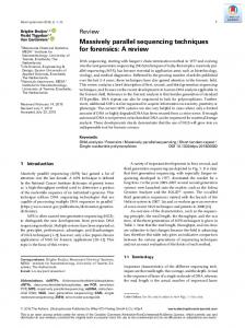
NAMD is a molecular dynamics program designed for high performance simulation of large biomolecular systems [7]. Each simulated timestep involves computing forces on each atom, and “integrating” them to update their positions. The forces are due to bonds, and electrostatic forces between atoms within a cut-off radius. NAMD is parallelized using Charm++ via a novel combination of force and spatial decomposition to generate enough parallelism for parallel machines with a large number of processors. Atoms are partitioned into cubes whose dimensions are slightly larger than the cutoff radius. For each pair of neighboring cubes, we assign a non-bonded force computation object, which can be independently mapped to any processor. The number of such objects is therefore 14 times (26/2 + 1 selfinteraction) the number of cubes. The cubes described above are represented in NAMD by objects called home patches. Each home patch is responsible for distributing coordinate data, retrieving forces, and integrating the equations of motion for all of the atoms in the cube of space owned by the patch. The forces used by the patches are computed by a variety of compute objects. There are several varieties of compute objects, responsible for computing the different types of forces (bond, electrostatic, constraint, etc.). On a given processor, there may be multiple “compute objects” that all need the coordinates from the same home patch. To eliminate duplication of communication, a “proxy” of the home patch is created on every processor where its coordinates are needed. The parallel structure of NAMD is shown in Fig. 1. Patches : Integration

Point to Point

Multicast

PME Angle Compute Objects

Pairwise Compute Objects Transposes

Asynchronous Reductions

Point to Point

Patches : Integration

Fig. 1. Parallel structure of NAMD

NAMD employs Charm++’s measurement-based load balancing. When a simulation begins, patches are distributed according to a recursive coordinate bisection 4

scheme, so that each processor receives a number of neighboring patches. All compute objects are then distributed to a processor owning at least one home patch. The framework measures the execution time of each compute object (the object loads), and records other (non-migratable) patch work as “background load.” After the simulation runs for several time-steps (typically several seconds to several minutes), the program suspends the simulation to trigger the initial load balancing. The strategy retrieves the object times and background load from the framework, computes an improved load distribution, and redistributes the migratable compute objects. The initial load balancer is aggressive, starting from the set of required proxies and assigning compute objects in order from larger to smaller, avoiding the need to create new proxies unless necessary. Once a good balance is achieved, atom migration changes very slowly. Another load balance is only needed after several thousand steps. We will present the performance optimizations we carried out with the help of Projections in a series of examples. The first two examples involve runs on the ASCI Red machine, while the rest are on PSC Lemieux [8].

3.1

Grainsize Analysis

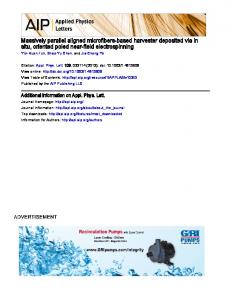
Fig. 2. Grainsize Distribution on ASCI Red

The benchmark application we used on ASCI Red machine was a 92,000 atom simulation, which took 57 seconds on one processor. Although it scaled reasonable well for few hundred processors, initial performance improvements stalled beyond 1,000 processors. One of the analysis using Projections logs we performed identified a cause. Most of the computation time was spent in force-computation objects. However, as shown in Figure 2, the execution time of computational objects was not uniform: it ranged from 1 to 41 msecs. The variation itself is not a problem (after all, Charm++’s load balancers are expected to handle that). However, having single objects with execution time of 40+ msecs, in a computation that should ideally run in 28 msecs on 2000 processors was clearly infeasible! This observation, 5

and especially the bimodal distribution of execution times, led us to examine the set of computational objects. We found the culprits to be those objects that correspond to electrostatic force computations between cubes that have a common face. If cubes touch only at corners, only a small fraction of atom-pairs will be within the cut-off distance and need to be evaluated. In contrast, those touching at faces have most within-cutoff pairs. Splitting these objects into multiple pieces led to a much improved grainsize distribution as shown in Fig. 2b. 3.2

Load Balancing

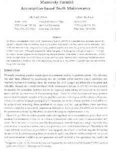
Fig. 3. Processor Utilization against Time on (a) 128 (b) 1024 processors

Dynamic load balancing was an important performance challenge for this application. The distribution of atoms over space is relatively non-uniform, and (as seen in the grainsize analysis above) the computational work is distributed quite non-uniformly among the objects. We used a measurement-based load balancing framework, which supports runtime load and communication tracing. The RTS admits different strategies (even during a single run) as plug-ins, which use the trace data. We used a specific greedy strategy[9]. For a 128-processor run, Projections visualization of the utilization graph (Fig. 3(a) ) confirmed that the load balancer worked very well: Prior to load balancing (at 82 seconds) relatively bad load imbalance led to utilization averaging to 65-70% in each cycle. However after load balancing, the next 16 steps ran at over 95% utilization. However, when the same strategy was used on 1024 processors, the results were not as satisfying (Fig. 3 (a)). In particular, (via a profile view not shown here) it became clear that the load on many processors was substantially different than what the load balancer had predicted. Since the greedy strategy used ignored existing placements of objects entirely (in order to create an unconstrained close-to-optimal mapping), it was surmised that the assumptions about background load (due to communication, for example) as well as cache performance were substantially different in the new context after the massive object migration induced by load balancer. Since the new mapping was expected to be close to optimal, we didn’t want to discard it. Instead, we added another load balancing phase immediately after the greedy reallocation, 6

Fig. 4. Processor Utilization after (a) greedy load balancing and (b) refining

which used a simpler “refinement” strategy: objects were moved only from the processors that were well above (say 5%) the average load. This ensured that the overall performance context (and communication behavior) was not perturbed significantly after refinement, and so the load-balancer predictions were in line with what happened. In Fig. 3(b), initial greedy balancer works from 157 through 160 seconds, leading to some increase in average utilization. Further, after the refinement strategy finished (within about .7 seconds) at around 161.6 seconds, we can see that utilization is significantly improved. Another view in Projections (Fig. 4), showing utilization as a function of processors for the time intervals before and after refinement, shows this effect clearly. Note that due to some quirks in the background load, several processors in the range between 500 and 600 were left underloaded by the greedy algorithm. The refinement algorithm did not change the load on those, since it focuses (correctly) only on overloaded processors: having a few underloaded processors doesn’t impact the performance much, but having even one overloaded processor slows the overall execution time. Here, we see that 4 overloaded processors (e.g, processor 508) were significantly overloaded before the refinement step, whereas the load is much much closer to the average after refinement. As a result, overall utilization across all processor rises from 45 to 60%.

3.3

Managing Stretches in Entry Methods

We successfully isolated and fixed the stretched (prolonged) entry method (handler) problem by the use of the timeline. This problem occured while running NAMD on a large number of processors on Lemieux. Figure 5 shows the timeline of NAMD on 1536 processors. Observe that processors 900 (processor 6 from the top) and 933 (processor 7) have handlers that last about 20-30 ms. This is clearly shown by the long superscript bar (colored in light grey) on top of the handler, which shows a send operation. Both the stretched handlers here block on a send operation. Nor7

mally these handlers should take about 2-3ms to finish, as shown by the remaining rectangles. Observe that the other superscript bars are just dots. We also noticed other stretches in the middle of entry methods (not shown in the figure). We believe these stretches were caused by a mis-tuned Elan library and operating system daemon interference. We now describe how we overcame this stretching problem.

Fig. 5. NAMD Run on 1536 processors

(a) Timeline showing Blocking Receives

(b) Profile View

Fig. 6. Namd on 3000 processors

Stretched Sends: The Charm/Converse [10] runtime system only makes calls to elan tportTxStart (equivalent of MPI Isend in Elan) which should be a short call [11,12]. But the entry methods were blocked in the send operations for tens of milliseconds. On looking at the Elan library source (and also working with Quadrics [13]), we found that this was a side effect of Elan software’s implementation of MPI message ordering. MPI message ordering requires that messages between two processors be ordered . In order to implement this ordering, the Elan system made a processor block on an elan tportTxStart if the rendezvous of any previous message had not been acknowledged, irrespective of the destination of that previous message. So in the presence of a hot-spot in the network, all processors that sent a message to the hot-spot would freeze. This could cascade leading to long stretches of even tens of milliseconds. We reported this to Quadrics, and obtained a fix for this problem. In the new Elan software, a message send only blocks if the previous rendezvous to its destination is unacknowledged, thus eliminating the stretched sends. 8

OS Daemon Stretches: Fixing the Elan software did not completely eliminate stretches, when applications used four processors on each node. NAMD simulation of the ATPase system takes about 12ms on 3000 processors. This time step is very close to the 10ms time quanta of the operating system. So if on any of the 3000 processors a file system daemon is scheduled, NAMD step time could become 22ms. Petrini et al. [14] have studied this issue of operating system interference in great detail. They present substantial performance gains for the SAGE application on ASCI-Q (a QsNet-Alpha [12] system similar to Lemieux) after certain file system daemons have been shutdown. We did not have control over the machine to do the system level experiments carried out by Petrini et al. However, we were still able to reduce and mitigate the impact of such interference with two mechanisms. First, NAMD uses a reduction in every step to compute the total energies. With Charm++, it was able to use an asynchronous reduction, whereby the next timestep doesn’t have to wait for the completion of the reduction. This gives the processors that were lagging behind due to a stretch an opportunity to catch up. Second, when a processor becomes idle, the receive module in the Converse communication layer blocks on a receive, instead of busywaiting. This enables the operating system to schedule daemons while the processor is sleeping. On receiving a message, there is an interrupt from the network interface which wakes the sleeping process up. The new timeline is presented in Figure 6(a), where there are no stretched entry methods. The dark-grey superscripted bars on top of the idle time implies that a processor is blocked on a receive. The profile view of selected 200 processors (0-49, 1000-1099, 2950-2999) is shown in Figure 6(b). The white area at the top represents idle time, which is quite substantial (25% or so). Timeline views (Figure 6(a)) show that load balance is still a possible issue (Processor 1039 appears overloaded as identified by profile view). Meanwhile, the communication subsystem still shows minor, but significant hiccups (a message sent from processor 1076 is not available on processor 1075 for over 10 msec after it is sent). These observations indicate that further performance improvement may be possible!

4

Performance Optimization of CPAIMD with Projections

Car-Parrinello ab initio molecular dynamics (CPAIMD) ([15–17]) can be used to study key chemical and biological processes. The CPAIMD methodology numerically solves Newton’s equations using forces derived from electronic structure calculations performed “on the fly” as the simulation proceeds. The parallelization of CPAIMD method is quite challenging. The parallelism of current implementations is restricted to the number of states, which is not enough to scale the problem to thousands of processors. This program also involves mul9

tiple parallel 3-D FFTs, which are known to be communication intensive due to the all-to-all nature of the communication they require. There are several other phases in the method that involve potentially large data movements, with relatively little computation. Parallelization of these phases necessitates complex trade-offs between memory, load balance, and communication costs. Such issues make scalability of the code a non-trivial problem to solve. The basic objects in the appliation are electron orbitals (or states), each of which represents fourier coefficients in 3D g-space (or reciprocal space). We parallelized this application using processor-virtualization, with each virtual processor being a plane of the g-space state. The g-space is however not very dense and only a fraction of the cube is non-zero. The initial mapping mapped the virtual processors for the planes uniformly among the processors. This initial mapping, generated a loadimbalance problem as highlighted by the “Overview” graph feature in Projections (Figure 7(a)) with 900 milliseconds per simulation step.

(a) Load imbalance in phases I and IX

(b) Final result with load-vectors

Fig. 7. Solving the problem of load imbalance on 1024 processors

A better mapping was then conceived by explicitly considering the load caused by each plane. This takes into account the number of non-zeroes in each plane, which is a more accurate estimate of the real work involved. The resulting performance gain is highlighted in Figure 7(b) with 480 milliseconds step time.

5

Performance Analysis on Next Generation Supercomputers

Parallel machines with an extremely large number of processors are now being designed and built. For example, the BlueGene (BG/L) machine being built by IBM will have 64,000 dual-processor nodes with 360 teraflops peak performance. Another more radical design from IBM, code-named Cyclops (BlueGene/C), had over one million floating point units, fed by 8 million instructions streams supported by individual thread units, targeting 1 petaflops of peak performance. 10

It is a significant challenge and require qualitative changes to the way we write parallel programs in order to exploit the enormous compute power, as well as the way we analyze the performance.

5.1

Experience of Projections on Extremely Large Parallel Machines

In order to evaluate both parallel applications and performance analysis tools on such supercomputers that are not even built yet, we have built a performance modeling and programming environment for petaflops-class supercomputers and the BlueGene machine [18]. It consists of a parallel simulator BigSim [19] that is capable of predicting parallel performance of applications on machines with a very large number of processors such as 64,000 processor BlueGene/L. We have employed essentially the same Projections framework for the BigSim simulator. The system can be used for 64K processors, but our experience with runs using Projections exposed a number of bottlenecks and limitations. For example, it is almost impractical to generate 64,000 trace log files. Reading and writing this large number of log files were expensive in terms of both I/O system overheads and the memory cost. We have implemented several schemes to extend current Projections capabilities to enhance it’s usefulness on such extremely large scale parallel machines. (1) Explore the more insightful information captured with more compact trace data representation in summary mode. For example, to understand the overall utilization over time, a sum of all utilizations per bin(interval) across all processors gives good information. An example is shown in Figure 8(a). (2) Instead of generating an unmanageable number of log files, a program can, at the end of its execution, perform a global reduction which collects and combines all trace data on all processors into one data file. (3) Generating detailed Projections log for every processor is infeasible but is desirable in some cases. We allow a user to specify a range of processors in interest and only trace logs of these subset of processors are generated. Further, at the time of visualizing the log files, only a subset of trace logs needs to be loaded into memory, other log files can be loaded on demand to reduce the memory cost and improve the speed. Similarly, users can start and stop instrumentation during specific phases of the program. This helps in reducing the log size. Case Study with MD on Extremely Large Machines: It is clearly quite challenging for molecular dynamics simulation to exploit the enormous compute power of next generation supercomputers. Applications need to face the grain size challenge that is much more significant than the one described in Section 3.1. For example, for a typical system simulation that takes about 6 seconds for one timestep on a sin11

gle processor, assuming perfect speedup, one would expect only 6 microseconds for each timestep on a 1 million processor machine. In the face of such extreme-scale supercomputers, NAMD, although shown to be able to scale to 3000 processors, is not ready due to its relatively coarse grained parallelism exploited. Given ER-GRE benchmark as an example, which is a system that contains 36,573 atoms, we calculate the number of cell-to-cell interactions (compute objects) using NAMD’s “one-away” decomposition strategy as described ˚ 3 , we have 8x8x8 numin Section 3. Considering a simulation space of 92x92x92 A ˚ which leads to only 7,168 cell-to-cell interber of Cells given the cutoff of 12 A, 1 actions to calculate. Considering that the BlueGene/L machine is about 64,000 nodes, the division would leave nodes idle even if interactions were delegated to a single node. To experiment with new parallelization strategy, we have developed an experimental prototype program called LeanMD that models the essential cutoff computations. In LeanMD, the “one-away” strategy is replaced with a “k-away” strategy. Instead of one cell representing the cutoff distance, in LeanMD three cells would span the cutoff distance. Therefore, in order to do the cutoff calculation, a cell must compute its interactions with every cell that is “three-away” in this scenario. Given the simulation example above, a three-away strategy would produce 13,824 cells and more than 2 million cell-to-cell interactions, a number of objects that is easily distributed across the 64,000 nodes of BlueGene/L.

(a) Average utilization per interval for LeanMD on 32,000 processors

(b) Distribution of processors based on load in ms

Fig. 8. LeanMD Projections Views

We have run LeanMD on our simulator on PSC Lemieux using the same ER-GRE benchmark, simulating the BlueGene/L of node size from 1K to 64K (full machine size). The simulation data can be used to carry out more detailed performance analysis using Projections. Figure 8(a) shows the average processor utilization as it 1

(8*8*8)*(26/2+1), since cell-to-cell forces are symmetric.

12

varies with time for a simulation on 32k simulated processors. The utilization stabilizes at about 50%, but rises and falls within each timestep. To further understand the scalability of LeanMD, we ran LeanMD from 1K to 64K simulated processors. The first row in Table 1 is the predicted speedup, normalized based on the 1000 processor time. The speedup saturates starting from 16k simulated processors. This could be due to either communication latencies, critical paths or load imbalance. To understand the saturation of the speedup we used the performance data to calculate the CPU load on each individual processor. Figure 8(b) shows a histogram of this data in the case of 16k simulated processors. Although about 6000 out of 16000 processors have a load of about 2ms, a few are seen to have a load as high as 11ms. This suggests that load balance is a major performance issue. To understand what portion of performance loss is explained by load imbalance alone, we calculate the avgLoad estimated speedup (P × maxLoad ) based on load imbalance loss alone (second row in Table 1) and compare it with simulated speedup. The closeness of both numbers confirms that load imbalance is the primary cause of performance loss. Only at 64K processors do the numbers deviate, indicating influence of other factors such as communication overhead or critical paths. Such detailed performance analysis is possible because of the rich performance trace data produced by the simulator. Processors

2000

4000

8000

16000

32000

64000

Predicted Speedup

1845

3384

6015

8658

14178

18180

Expected Speedup 1865 3412 6242 8635 Table 1 Predicted vs. expected speedup, normalized based on 1000

13916

19936

6

Conclusion and Future Work

We introduced Projections, a performance analysis tool used in conjunction with the Charm++ parallel programming system. The Projections tracing system automatically creates execution traces, in a compact but useful “summary” mode, or a detailed “log” mode. We showed how the analysis system, and various views it presents, were used in scaling a production quality application NAMD to 3,000 processors and 1 TF, and an ongoing CPAIMD project to 1,500 processors. This experience has helped us identify and add additional capabilities Projections in order to respond to the challenges of extremely large machines. We now plan to further extend the Projections framework to allow users to add such capabilities by expressing simple queries or predicates they want evaluated. The relatively large number and size of trace files in the log mode has led us to create an intermediate summary mode that preserves as much useful information as possible while reducing the amount of data significantly. Linking the performance visualization system’s views to source code information, as done in SvPablo [20], 13

will also be another useful extension. We have already added preliminary features that use performance counters which will be used in an integrated automatic analysis system. We are currently also in the process of extending these features to AMPI. We also continue to seek methods to improve the scalability of Projections, allowing it to visualize logs from a very large number of processors.

References

[1] L. V. Kale, S. Krishnan, Charm++: Parallel Programming with Message-Driven Objects, in: G. V. Wilson, P. Lu (Eds.), Parallel Programming using C++, MIT Press, 1996, pp. 175–213. [2] C. Huang, O. Lawlor, L. V. Kalé, Adaptive MPI, in: Proceedings of the 16th International Workshop on Languages and Compilers for Parallel Computing (LCPC 03), College Station, Texas, 2003. [3] L. V. Kalé, The virtualization model of parallel programming : Runtime optimizations and the state of art, in: LACSI 2002, Albuquerque, 2002. [4] O. S. Lawlor, L. V. Kalé, Supporting dynamic parallel object arrays, Concurrency and Computation: Practice and Experience 15 (2003) 371–393. [5] Upshot, http://www-fp.mcs.anl.gov/ lusk/upshot. [6] M. Heath, J. Etheridge, Visualizing the Performance of Parallel Programs, IEEE Software. [7] J. C. Phillips, G. Zheng, S. Kumar, L. V. Kalé, NAMD: Biomolecular simulation on thousands of processors, in: Proceedings of SC 2002, Baltimore, MD, 2002. [8] Lemieux, http://www.psc.edu/machines/tcs/lemieux.html. [9] L. Kalé, R. Skeel, M. Bhandarkar, R. Brunner, A. Gursoy, N. Krawetz, J. Phillips, A. Shinozaki, K. Varadarajan, K. Schulten, NAMD2: Greater scalability for parallel molecular dynamics, Journal of Computational Physics 151 (1999) 283–312. [10] L. V. Kale, M. Bhandarkar, N. Jagathesan, S. Krishnan, J. Yelon, Converse: An Interoperable Framework for Parallel Programming, in: Proceedings of the 10th International Parallel Processing Symposium, 1996, pp. 212–217. [11] S. Kumar, L. V. Kale, Opportunities and Challenges of Modern Communication Architectures: Case Study with QsNet, Tech. Rep. 03-15, Parallel Programming Laboratory, Department of Computer Science, University of Illinois at UrbanaChampaign (2003). [12] F. Petrini, S. Coll, E. Frachtenberg, A. Hoisie, Performance Evaluation of the Quadrics Interconnection Network, to appear, Journal of Cluster Computing (2002). URL citeseer.nj.nec.com/petrini01performance.html [13] Quadrics Ltd., http://www.quadrics.com.

14

[14] S. P. Darren J. Kerbyson, Fabrizio Petrini, The Case of the Missing Supercomputer Performance: Achieving Optimal Performance on the 8,192 Processors of ASCI Q, in: Supercomputing 2003, 2003. [15] G. Galli, M. Parrinello, Ab-initio molecular dynamics: Principles and practical inplementation, Computer simulation in chemical physics, NATO ASI Series C 397 (1993) 261. [16] M. C. Payne, M. P. Teter, D. C. Allan, T. A. Arias, J. D. Joannopoulos, Rev. Mod. Phys. 64 (1992) 1045. [17] M. E. Tuckerman, Ab initio molecular dynamics: Basic concepts, current trends and novel applications, J. Phys. Condensed Matter 14 (2002) R1297. [18] G. Zheng, T. Wilmarth, O. S. Lawlor, L. V. Kalé, S. Adve, D. Padua, Performance modeling and programming environments for petaflops computers and the blue gene machine, in: NSF Next Generation Systems Program Workshop, 18th International Parallel and Distributed Processing Symposium(IPDPS), Santa Fe, New Mexico, 2004. [19] G. Zheng, G. Kakulapati, L. V. Kalé, Bigsim: A parallel simulator for performance prediction of extremely large parallel machines, in: 18th International Parallel and Distributed Processing Symposium (IPDPS), Santa Fe, New Mexico, 2004. [20] L. DeRose, D. A. Reed, Svpablo: A multi-language architecture-independent performance analysis system, in: Proceedings of the International Conference on Parallel Processing (ICPP), 1999. [21] M. Bhandarkar, L. V. Kale, E. de Sturler, J. Hoeflinger, Object-Based Adaptive Load Balancing for MPI Programs, in: Proceedings of the International Conference on Computational Science, San Francisco, CA, LNCS 2074, 2001, pp. 108–117. [22] V. Adve, J. Mellor-Crummey, M. Anderson, K. Kennedy, J.-C. Wang, D. Reed, An Integrated Compilation and Performance Analysis Environment for Data Parallel Programs, in: Proceedings of Supercomputing’95, 1995. [23] A. Sinha, L. V. Kale, Towards Automatic Peformance Analysis, in: Proceedings of International Conference on Parallel Processing, Vol. III, 1996, pp. 53–60.

15