other words multiview hyperspectral photogrammetric imagery, and each object point appears in ... al., 2017) and the Cubert UHD Firefly snapshot hyperspectral.
The International Archives of the Photogrammetry, Remote Sensing and Spatial Information Sciences, Volume XLII-3, 2018 ISPRS TC III Mid-term Symposium “Developments, Technologies and Applications in Remote Sensing”, 7–10 May, Beijing, China
OPTIMIZING RADIOMETRIC PROCESSING AND FEATURE EXTRACTION OF DRONE BASED HYPERSPECTRAL FRAME FORMAT IMAGERY FOR ESTIMATION OF YIELD QUANTITY AND QUALITY OF A GRASS SWARD R. Näsi1, N. Viljanen1, R. Oliveira1, J. Kaivosoja2, O. Niemeläinen2, T. Hakala1, L. Markelin1, S. Nezami1, J. Suomalainen1 , E. Honkavaara1* 1
National Land Survey of Finland, Finnish Geospatial Research Institute FGI, FI-00521 Helsinki, Finland - (roope.nasi, niko.viljanen, raquel.alvesdeoliveira, teemu.hakala, lauri.markelin, somayeh.nezami, juha.suomalainen, eija.honkavaara)@nls.fi 2 Natural Resources Institute Finland - LUKE, Latokartanonkaari 9, FI-00790 Helsinki, Finland - (jere.kaivosoja, oiva.niemelainen)@luke.fi Commission III, WG III/4
KEY WORDS: Hyperspectral, Photogrammetry, Calibration, Feature, Estimation
ABSTRACT: Light-weight 2D format hyperspectral imagers operable from unmanned aerial vehicles (UAV) have become common in various remote sensing tasks in recent years. Using these technologies, the area of interest is covered by multiple overlapping hypercubes, in other words multiview hyperspectral photogrammetric imagery, and each object point appears in many, even tens of individual hypercubes. The common practice is to calculate hyperspectral orthomosaics utilizing only the most nadir areas of the images. However, the redundancy of the data gives potential for much more versatile and thorough feature extraction. We investigated various options of extracting spectral features in the grass sward quantity evaluation task. In addition to the various sets of spectral features, we used photogrammetry-based ultra-high density point clouds to extract features describing the canopy 3D structure. Machine learning technique based on the Random Forest algorithm was used to estimate the fresh biomass. Results showed high accuracies for all investigated features sets. The estimation results using multiview data provided approximately 10% better results than the most nadir orthophotos. The utilization of the photogrammetric 3D features improved estimation accuracy by approximately 40% compared to approaches where only spectral features were applied. The best estimation RMSE of 239 kg/ha (6.0%) was obtained with multiview anisotropy corrected data set and the 3D features.
1. INTRODUCTION The use of light-weight 2D format hyperspectral (HS) imagers operable from unmanned aerial vehicles (UAV or drone) has become common in various remote sensing tasks. Examples of these cameras include the Rikola camera of Senop Ltd. based on tuneable Fabry-Pérot interferometer (FPI) (Mäkynen et al., 2011; Honkavaara et al., 2013; Oliveira et al., 2016; Jakob et al., 2017) and the Cubert UHD Firefly snapshot hyperspectral camera (Aasen et al., 2015; Yang et al., 2017). Their advantages in comparison to the commonly used pushbroom scanners are that they capture stereoscopic data and do not require complicated orientation processing supported by the GNSS/IMU direct orientation techniques (Mäkynen et al., 2011; Honkavaara et al., 2013). In the 2D format imaging setup, the area of interest is covered by an image block that has multiple overlapping images. Typically, each object point appears in 10-30 individual hypercubes. The common practice is to calculate hyperspectral orthomosaics thus only single spectra for each pixel is used. However, the image redundancy gives various additional opportunities for feature extraction. Images can be mosaicked, to capture single reflectance value for each ground pixel, or multiple reflectance spec1tra can be taken from the overlapping images, and additional features (e.g. anisotropy, standard deviation, etc.) can be calculated from the multiview observations. In addition, dense point clouds can be created
from the dataset in order to extract features describing the canopy 3D structure, such as height average or standard deviation. It is expected that these different information could be utilized to improve classification and estimation processes. For example, previous studies by Roosjen et al. (2016) showed that the anisotropy of barley, winter wheat and potato in two measurement dates was different, and could potentially be used as a signal in operational remote sensing. Recently, Roosjen et al. (2018) used the PROSAIL radiative transfer tool to estimate the leaf area index and the leaf chlorophyll content using the nadir and multi-angular data collected by the UAV. Simulated and empirical results showed that the estimates improved when adding multi-angular observations to the estimation process. The drone-based photogrammetric point clouds have also shown potential in agricultural crop biomass estimation (eg. Bendig et al., 2013; Li et al., 2016; Näsi et al., 2017). The objective of this investigation was to evaluate various options of extracting features from RGB and HS 2D frame format image datasets. An experimental assessment was carried out in the case of fresh biomass estimation of grass sward using a Random Forest estimator.
* Corresponding author
This contribution has been peer-reviewed. https://doi.org/10.5194/isprs-archives-XLII-3-1305-2018 | © Authors 2018. CC BY 4.0 License.
1305
The International Archives of the Photogrammetry, Remote Sensing and Spatial Information Sciences, Volume XLII-3, 2018 ISPRS TC III Mid-term Symposium “Developments, Technologies and Applications in Remote Sensing”, 7–10 May, Beijing, China
2. MATERIALS AND METHODS 2.1 Test area Experiments were conducted in a silage production field at the Natural Resources Institute Finland (LUKE) research farm, located in the municipality of Jokioinen in South-West Finland (approximately 60°48′N, 23°30′E). The size of the experimental area was approximately 50 m by 20 m (Figure 1). The experimental set up was a split plot design with four replicates. The fertilizer treatment was divided into 24 main plots (plot size 12 m x 3 m), and the harvesting time was in 96 sub-plots of size of 1.5 m by 3 m. The idea of the experimental set up was to generate great variation in the study sward. The experiment had six different nitrogen fertilizer application rates (0, 50, 75, 100, 125 and 150 kg N/ha) and used four harvesting dates from 6.6.2017 to 28.6.2017. In this study only the dataset captured in 6.6.2017 was used, therefore, we had altogether 24 reference plots of size of 1.5 m by 3 m, having six different nitrogen fertilizer levels with four replicates. Reference measurements included grass height, fresh and dry matter yield, and feeding quality characteristics. The measured fresh biomass values varied from 1022 to 5975 kg/ha, where the lowest amount was detected from a sub-plot without nitrogen fertilizer and the highest from a sub-plot with the maximum nitrogen fertilization level.
Five permanent ground control points (GCPs) were installed in corners and center of the block. They were black painted plywood boards of size 0.5 m by 0.5 m, with a white painted circle with diameter of 0.3 m. GCPs were measured with Trimble R10 RTK DGNSS within 0.03 m horizontal and 0.04 m vertical accuracy. For reflectance transformation purposes, three reflectance panels of size of 1 m by 1 m with nominal reflectivity of 0.03, 0.1 and 0.5 were set up next to the area with the grassplots. The flying altitude was 50 m giving the GSDs of 5 cm for the hyperspectral data and less than 1 cm for the RGB data. The flying speed was 1 m/s and distance between collected 4 flight lines was 8 m resulting 85% forward and side overlaps for FPI images. Theoretically, this provides 32 multiview observations for each object point.
Figure 2. Data capture using the FGI quadrocopter drone.
Figure 1. RGB orthomosaic from the test area in 6 June, 2018 and locations of 24 sample plots and flight trajectory.
Band 1 L0 [nm] 512.3 FWHM [nm] 14.81
2 514.8 17.89
3 520.4 20.44
4 527.5 21.53
5 542.9 19.50
6 550.6 20.66
7 559.7 19.56
8 569.9 22.17
9 579.3 17.41
10 587.9 17.56
Band 11 L0 [nm] 595.9 FWHM [nm] 21.35
12 604.6 20.24
13 613.3 25.30
14 625.1 27.63
15 637.5 24.59
16 649.6 27.86
17 663.8 26.75
18 676.9 27.00
19 683.5 28.92
20 698.0 24.26
Band 21 L0 [nm] 705.5 FWHM [nm] 24.44
22 711.4 25.12
23 717.5 27.45
24 723.8 27.81
25 738.1 26.95
26 744.9 25.56
27 758.0 27.78
28 771.5 27.61
29 800.5 23.82
30 813.4 28.28
Band 31 L0 [nm] 827.0 FWHM [nm] 26.61
32 840.7 26.85
33 852.9 27.54
34 865.3 28.29
35 879.6 25.89
36 886.5 23.69
Table 1. Spectral settings of the hyperspectral camera. L0: center wavelength; FWHM: full width at half maximum.
2.2 Data capture campaign
2.3 Data processing chain
The Finnish Geospatial Research Institute’s (FGI’s) drone was utilized for collecting the remote sensing datasets on 6 June 2017 at 15:30 local time (Figure 2). The sun zenith was 51.3° was and azimuth was 217.9°. Weather conditions were mostly sunny and windless. The frame of FGI’s drone was Gryphon Dynamics quadcopter with detachable arms and it was equipped with Pixhawk autopilot with ArduPilot APM Copter 3.4 firmware. The drone was equipped with a positioning system consisting of an NV08C-CSM L1 GNSS receiver, a Vectornav VN-200 IMU and a Rasberry Pi single-board computer. The sensor payload included an RGB digital camera, Sony A7R, and a hyperspectral camera based on a tuneable Fabry Pérot interferometer (FPI), operating in the visible to near-infrared spectral range (500-900 nm) (Mäkynen et al., 2011; Honkavaara et al., 2013). The FPI camera is lightweight, frame format hyperspectral imager operating in time-sequential principle, collecting spectral bands with 648 by 1024 pixels. In this study, we used the mode with 36 bands (Table 1).
The approach in the data processing was to generate ultra-dense point clouds using the RGB datasets and to calculate image mosaics and other spectral features using the HS data sets. The datasets were processed using the processing line developed at the FGI (Honkavaara et al., 2013, 2017, 2018; Näsi et al., 2018; Nevalainen et al., 2017). The steps are the following: 1. Applying laboratory calibration corrections to the images. 2. Determination of the geometric imaging model, including interior and exterior orientations of the images. 3. Using dense image matching to create an ultra-high density photogrammetric digital surface model (DSM). 4. Determination of a radiometric imaging model to transform the digital number (DNs) data to reflectance. 5. Calculating the radiometric output products 6. Extracting spectral and other image and 3D structural features. 7. Estimation of grass parameters.
This contribution has been peer-reviewed. https://doi.org/10.5194/isprs-archives-XLII-3-1305-2018 | © Authors 2018. CC BY 4.0 License.
1306
The International Archives of the Photogrammetry, Remote Sensing and Spatial Information Sciences, Volume XLII-3, 2018 ISPRS TC III Mid-term Symposium “Developments, Technologies and Applications in Remote Sensing”, 7–10 May, Beijing, China
The processing was divided to the geometric (steps: 2, 3) and radiometric (steps 1, 4, 5) processing steps. The further procedures for feature extraction and estimation are presented in Section 2.4. Agisoft Photoscan Professional (version 1.3.5) was used for the photogrammetric processing, which involved image orientation estimation and DSM generation. The RGB images were processed separately, and the three reference bands of the FPI images were processed in a combined processing with the RGB images. The band registration for the rest of the bands of the FPI images was carried out using the approach developed by Honkavaara et al. (2017). The object point cloud can be produced from the FPI images, but in this study we used the RGB camera to calculate an ultra-high resolution DSM with 1 cm GSD.
without (processing levels 3a, 4a) 3D features. In processing level 5, sample-wise BRDF-model parameters from each band were used as features. Estimation and validation were done using the Random Forest (RF) estimation (Breiman, 2001) implemented in the software Weka (Weka 3.8.1, University of Waikato). The RF method was used to estimate grass sward yield quantity (fresh above-ground biomass) parameter. To assess the prediction accuracy during the estimation of biomass for grass we used 2/3 of the samples to train and 1/3 of the samples to test the model. The estimation accuracy was quantified using Correlation Coefficients and Root Mean Square Error (RMSE).
3. RESULTS 3.1 Radiometric processing results
The in-house rigorous radiometric processing software, radBA, was used for the radiometric processing of the FPI images (Honkavaara et al., 2013; Honkavaara and Khoramshahi, 2018). The processing used different processing levels to create the mosaics: 1. Uncorrected nadir mosaic. Mosaics were created using the most nadir parts of the images. Reflectance calibration was carried out using the empirical line (EL) method with panels (Smith and Milton, 1999). 2. Corrected nadir-mosaic. Mosaics were created using the most nadir parts of the images applying the irradiance and anisotropy corrections, as well as reflectance calibration using the panels. 3. Multiview hemispherical directional reflectance factor (HDRF) point cloud. Reflectance was taken from each image where the sample point appeared. Reflectance calibration was carried out using the EL-method. 4. Anisotropy corrected multiview reflectance point cloud. Reflectance was taken from each image where the sample point appeared. The irradiance and anisotropy corrections were applied and the reflectance calibration was performed using panels. 5. Sample-wise bidirectional reflectance distribution function (BRDF) model parameters. The Walthall’s (Walthall et al., 1985; Honkavaara and Khoramshahi, 2018) BRDF model was estimated for each sample point and the parameters were used as the features. In this model, the parameter b1 represents the impact of the zenith view angle, b2 accounts for the azimuth angle difference of the sun and viewing directions and the b3 represents the reflectance at nadir view direction.
The illumination conditions during the data collection were clear and sunny during three first flight lines and partially cloudy during the last flight line. We used only the three first lines in the estimations to obtain homogeneous data quality. Orthophoto mosaics of processing levels 1 and 2 (Uncorrected and corrected nadir mosaics) are shown in Figure 3. The homogeneity (coefficient of variation) was on the level of 10% in the overlapping images (Figure 4), and the radiometric processing improved the homogeneity only slightly. The ortophoto mosaic was visually uniform even without anisotropy correction because the view zenith angles in the most nadir mosaics were less than 3° due to the high overlaps thus the resulting anisotropy effects were minor.
(a)
(b)
2.4 Feature extraction and estimation Reflectance values from 36 bands were extracted and used as spectral features. Based on processing levels (section 2.3) the average reflectance value of the window, with a size of 50 cm x 50 cm, were extracted from the most nadir mosaics (processing levels: 1-2) or using each image where point appeared (processing levels: 3-4). Furthermore, 3D features based on canopy height model (CHM), which was created using the RGB camera-based 3D photogrammetric point cloud, were extracted for the plots; the features included the average, median, minimum, maximum, standard deviation and percentiles (70, 80, 90) of the canopy heights. The estimation in multiview approaches were performed with (processing level 3b, 4b) and
Figure 3. (a) Uncorrected and (b) corrected orthophoto mosaics, bands 790.85, 668.97 and 537.48nm.
This contribution has been peer-reviewed. https://doi.org/10.5194/isprs-archives-XLII-3-1305-2018 | © Authors 2018. CC BY 4.0 License.
1307
The International Archives of the Photogrammetry, Remote Sensing and Spatial Information Sciences, Volume XLII-3, 2018 ISPRS TC III Mid-term Symposium “Developments, Technologies and Applications in Remote Sensing”, 7–10 May, Beijing, China
b3 0.50
0.40
n000
0.30
n050
0.20
n075 n100
0.10
n125
0.00 500
600
700 800 Wavelength (nm)
900
n150
Figure 5. BRDF parameters calculated using all sample points of specific nitrogen fertilization level: (a) b1, (b) b2 and (c) b3. n000 to n150 represent the nitrogen fertilization levels. Figure 4. Uniformity of the image mosaic. sd_refl_orig: coefficient of variation of the origninal mosaic; sd_refl_fin: coefficient of variation of the corrected mosaic.
3.2 BRDF estimation First we estimated three BRDF parameters for each nitrogen fertilization level using all sample points (Figure 5). In these plots, the wavelength dependency is clearly visible and also the nitrogen fertilization levels impacted the parameters. (a)
b1
In order to investigate how different fertilization levels impacted the modelled reflectance and anisotropy, we calculated the BRDF and anisotropy factors (Honkavaara and Khromashahi, 2018) for different nitrogen fertilization levels for red (L0=649.60 nm) and NIR (L0=800.50 nm) bands at the solar principal plane (Figure 6). In these plots, we see clearly the different behaviour of different spectral ranges; in the red band, the low reflectance in the forward scattering direction is due to the chlorophyll absorption and due to the fact that the shadowed parts of the canopy is seen (Figure 6a). In the case of the NIR band, the BRDF had a bowl shape which is the expected behaviour (Figure 6b). The results regarding the behaviour of different spectral ranges are consistent with previous results by Roosjen et al. (2016).
0.5
(a)
0.4
0.14
0.3
n050
0.12
0.2
n075
n100
0.1
n125
0 -0.1
500
600
700
800
900
n150
Wavelength (nm)
BRDF at princ. Plane
n000
0.1
n000
0.08
n050
0.06
n075
0.04
n100
0.02
n125
0 -40
(b)
b2 0.14 0.12 0.1 0.08 0.06 0.04 0.02 0
-20 0 20 View zenith angle (deg)
40
n150
(b) n000
n075 n100 n125 500
600
700 800 Wavelength (nm)
900
n150
0.5 BRDF at princ. Plane
n050
0.4 n000
0.3
n050
0.2
n075
0.1
n100 n125
0 -40
(c)
-20 0 20 View zenith angle (deg)
40
n150
Figure 6. BRDF at solar principal plane for (a) red band and (b) NIR band. n000 to n150 represent the nitrogen fertilization levels.
This contribution has been peer-reviewed. https://doi.org/10.5194/isprs-archives-XLII-3-1305-2018 | © Authors 2018. CC BY 4.0 License.
1308
The International Archives of the Photogrammetry, Remote Sensing and Spatial Information Sciences, Volume XLII-3, 2018 ISPRS TC III Mid-term Symposium “Developments, Technologies and Applications in Remote Sensing”, 7–10 May, Beijing, China
(a)
Processing level
Anisotropy factor
1.8 1.6 n000
1.4
n050
1.2
n075
1
n100
0.8
n125
0.6
n150 -40
-20 0 20 View zenith angle (deg)
40
(b)
Anisotropy factor
1.8 1.6 1.4
n000
1.2
n050
1
n075
n100
0.8
n125
0.6 -40
-20 0 20 View zenith angle (deg)
40
n150
Figure 7. Anisotropy at solar principal plane for (a) red band and (b) NIR band. n000 to n150 represent the nitrogen fertilization levels.
3.3 Estimation results The RF algorithm was used to estimate fresh biomass yield. The results were good for all selected feature sets (Table 2). In processing the levels 1 and 2, spectral features were extracted from most-nadir images. The difference between these sets were that only in the processing level 2, the irradiance and anisotropy corrections were applied to the mosaic. The estimation performance was similar, which was expected because the mosaics were uniform in both cases (Figure 3). The estimation results using multiview data on processing levels 3a and 4a provided approximately 10% better results than the most nadir approaches (1-2). Adding the 3D features improved the estimation accuracies approximately 40% (3b, 4b) based on RMSE values. The sample-wise BRDF parameters were extracted for 15 samples which had BRDF parameters for every band. In this case correlation coefficient was 0.967 and b3 parameters (Figure 5) were most important features based on RF algorithm. The estimation accuracies were at the same level as in the other cases that did not have the 3D features. The best estimation RMSE was 239 kg/ha (6.0%) with the multiview anisotropy corrected mosaic and the 3D features. This can be considered as very good accuracy level.
1 Uncorrected nadir mosaic 2 Corrected nadir mosaic 3a Multiview HDRF mosaic 3b Multiview HDRF point cloud 4a Multiview anistropy corrected mosaic 4b Multiview anistropy corrected point cloud 5 Sample-wise BRDF parameters
Corr. coeff. 0.985
RMSE (kg/ha) 435.1
RMSE (%) 11.1
0.985
534.0
13.6
0.959
444.5
11.3
0.987
261.4
6.6
0.968
390.8
9.9
0.989
236.9
6.0
0.967
445.7
13.0
Table 2. The fresh biomass estimation results (Corr. coeff.= Pearson correlation coefficient, RMSE= root-mean-square error in kg/ha and %) for different processing levels: 1 Uncorrected nadir mosaic, 2 Corrected nadir mosaic, 3a Multiview HDRF mosaic, 3b Multiview HDRF point cloud, 4a Multiview anisotropy corrected mosaic, 4b Multiview anisotropy corrected point cloud and 5 Sample-wise BRDF parameters. 4. CONCLUSIONS This study evaluated different options to extract features of a dataset based on 2D frame format hyperspectral image block and a photogrammetric ultra-high resolution canopy height model. The estimation task was the fresh biomass yield estimation of the grass sward. The Random Forest algorithm was used to estimate fresh biomass amount successfully for all feature sets. The preliminary estimation results using multiview data showed improvements of about 10% in comparison to the case using the most nadir orthophoto mosaic. The use of photogrammetric 3D features improved estimation accuracy up to 40% in comparison to the approaches where only spectral features were applied. The utilization of the bidirectional reflectance distribution function (BRDF) parameters in the estimation process did not improve the results in our preliminary results. However, the BRDF effects (anisotropy factors) at the maximum view angles were up to 60% and different nitrogen fertilization levels provided different BRDF-parameters, which suggested that further considerations of the utilization of these parameters are necessary. Further interesting test cases will be the estimation of other parameters, such as grass quality, e.g. the digestibility.
ACKNOWLEDGEMENTS The authors would like to acknowledge funding by Business Finland DroneKnowledge-project (Dnro 1617/31/2016).
This contribution has been peer-reviewed. https://doi.org/10.5194/isprs-archives-XLII-3-1305-2018 | © Authors 2018. CC BY 4.0 License.
1309
The International Archives of the Photogrammetry, Remote Sensing and Spatial Information Sciences, Volume XLII-3, 2018 ISPRS TC III Mid-term Symposium “Developments, Technologies and Applications in Remote Sensing”, 7–10 May, Beijing, China
REFERENCES Aasen, H., Burkart, A., Bolten, A., Bareth, G., 2015. Generating 3D hyperspectral information with lightweight UAV snapshot cameras for vegetation monitoring: From camera calibration to quality assurance. ISPRS Journal of Photogrammetry and Remote Sensing, 108(2015), pp. 245–259. Bendig, J., Bolten, A., Bareth, G., 2013. UAV-based imaging for multi-temporal, very high Resolution Crop Surface Models to monitor Crop Growth Variability. PhotogrammetrieFernerkundung-Geoinformation, 2013(6), pp. 551-562. Breiman, L., 2001. Random forests. Machine learning, 45(1), pp. 5-32. Honkavaara, E., Saari, H., Kaivosoja, J., Pölönen, I., Hakala, T., Litkey, P., Mäkynen, J., Pesonen, L., 2013. Processing and Assessment of Spectrometric, Stereoscopic Imagery Collected Using a Lightweight UAV Spectral Camera for Precision Agriculture. Remote Sensing, 5(10), pp. 5006–5039. Honkavaara, E., Rosnell, T., Oliveira, R., Tommaselli, A., 2017. Band registration of tuneable frame format hyperspectral UAV imagers in complex scenes. ISPRS Journal of Photogrammetry and Remote Sensing, 134(2017), pp. 96–109. Honkavaara, E., Khoramshahi, E., 2018. Radiometric Correction of Close-Range Spectral Image Blocks Captured Using an Unmanned Aerial Vehicle with a Radiometric Block Adjustment. Remote Sensing, 10(2), 256, doi.org/10.3390/rs10020256. Jakob, S., Zimmermann, R., Gloaguen, R., 2017. The Need for Accurate Geometric and Radiometric Corrections of DroneBorne Hyperspectral Data for Mineral Exploration: MEPHySTo—A Toolbox for Pre-Processing Drone-Borne Hyperspectral Data. Remote Sensing, 9(1), 88, doi.org/10.3390/rs9010088. Li, W., Niu, Z., Chen, H., Li, D., Wu, M., Zhao, W., 2016. Remote estimation of canopy height and aboveground biomass of maize using high-resolution stereo images from a low-cost unmanned aerial vehicle system. Ecological Indicators, 67(2016), pp. 637-648, doi.org/10.1016/j.ecolind.2016.03.036.
doi.org/10.5194/isprs-archives-XLII-3-W3-137-2017. Näsi, R., Honkavaara, E., Blomqvist, M., LyytikäinenSaarenmaa, P., Hakala, T., Viljanen, N., Holopainen, M., 2018. Remote sensing of bark beetle damage in urban forests at individual tree level using a novel hyperspectral camera from UAV and aircraft. Urban Forestry & Urban Greening. 30(2018), pp. 72–83, doi.org/10.1016/j.ufug.2018.01.010. Oliveira, R.A., Tommaselli, A.M. and Honkavaara, E., 2016. Geometric calibration of a hyperspectral frame camera. The Photogrammetric Record, 31(155), pp. 325-347, doi.org/10.1111/phor.12153. Roosjen, P., Suomalainen, J., Bartholomeus, H., Clevers, J., 2016. Hyperspectral Reflectance Anisotropy Measurements Using a Pushbroom Spectrometer on an Unmanned Aerial Vehicle—Results for Barley, Winter Wheat, and Potato. Remote Sensing, 8(11), 909, doi.org/10.3390/rs8110909. Roosjen, P.P.J., Brede, B., Suomalainen, J.M., Bartholomeus, H.M., Kooistra, L., Clevers, J.G.P.W., 2018. Improved estimation of leaf area index and leaf chlorophyll content of a potato crop using multi-angle spectral data – potential of unmanned aerial vehicle imagery. Int. J. Appl. Earth Obs. Geoinformation, 66(2018), pp. 14–26, doi.org/10.1016/j.jag.2017.10.012. Smith, G. M., Milton, E. J., 1999. The use of the empirical line method to calibrate remotely sensed data to reflectance. International Journal of remote sensing, 20(13), pp. 26532662. Walthall, C. L., Norman, J. M., Welles, J. M., Campbell, G., Blad, B. L., 1985. Simple equation to approximate the bidirectional reflectance from vegetative canopies and bare soil surfaces. Applied Optics, 24(3), pp. 383-387. Yang, G., Li, C., Wang, Y., Yuan, H., Feng, H., Xu, B., Yang, X., 2017. The DOM Generation and Precise Radiometric Calibration of a UAV-Mounted Miniature Snapshot Hyperspectral Imager. Remote Sensing, 9(7), 642, doi.org/10.3390/rs9070642.
Mäkynen, J., Holmlund, C., Saari, H., Ojala, K., Antila, T., 2011. Unmanned aerial vehicle (UAV) operated megapixel spectral camera. In: Proceedings Volume 8186, Electro-Optical Remote Sensing, Photonic Technologies, and Applications V, 81860Y (2011), doi: 10.1117/12.897712. Nevalainen, O., Honkavaara, E., Tuominen, S., Viljanen, N., Hakala, T., Yu, X., Hyyppä, J., Saari, H., Pölönen, I., Imai, N.N., Tommaselli, A.M.G., 2017. Individual Tree Detection and Classification with UAV-Based Photogrammetric Point Clouds and Hyperspectral Imaging. Remote Sensing, 9(3), 185, doi.org/10.3390/rs9030185. Näsi, R., Viljanen, N., Kaivosoja, J., Hakala, T., Pandžić, M., Markelin, L., Honkavaara, E., 2017. Assessment of various remote sensing technologies in biomass and nitrogen content estimation using an agricultural test field. In: International Archives of the Photogrammetry, Remote Sensing and Spatial Information Sciences, Vol. XLII-3/W3, pp. 137-141,
This contribution has been peer-reviewed. https://doi.org/10.5194/isprs-archives-XLII-3-1305-2018 | © Authors 2018. CC BY 4.0 License.
1310