The International Archives of the Photogrammetry, Remote Sensing and Spatial Information Sciences, Volume XLII-1/W1, 2017 ISPRS Hannover Workshop: HRIGI 17 – CMRT 17 – ISA 17 – EuroCOW 17, 6–9 June 2017, Hannover, Germany
AN ENHANCED ALGORITHM FOR AUTOMATIC RADIOMETRIC HARMONIZATION OF HIGH-RESOLUTION OPTICAL SATELLITE IMAGERY USING PSEUDOINVARIANT FEATURES AND LINEAR REGRESSION Maximilian Langheinrich*a, Peter Fischera, Markus Probeckb, Gernot Rammingerb, Thomas Wagnerb, Thomas Kraußa a
Remote Sensing Technology Institute, German Aerospace Center (DLR) Münchner Str. 20, 82234 Wessling, Germany (Maximilian.Langheinrich, Peter.Fischer, Thomas.Krauss)@dlr.de b GAF AG Arnulfstr. 199, 80634 München, Germany
[email protected]
KEY WORDS: Radiometric Harmonization, Pseudo-Invariant Features, Sentinel-2, Remote Sensing, Copernicus, GIO, HRL Forest
ABSTRACT: The growing number of available optical remote sensing data providing large spatial and temporal coverage enables the coherent and gapless observation of the earth’s surface on the scale of whole countries or continents. To produce datasets of that size, individual satellite scenes have to be stitched together forming so-called mosaics. Here the problem arises that the different images feature varying radiometric properties depending on the momentary acquisition conditions. The interpretation of optical remote sensing data is to a great extent based on the analysis of the spectral composition of an observed surface reflection. Therefore the normalization of all images included in a large image mosaic is necessary to ensure consistent results concerning the application of procedures to the whole dataset. In this work an algorithm is described which enables the automated spectral harmonization of satellite images to a reference scene. As the stable and satisfying functionality of the proposed algorithm was already put to operational use to process a high number of SPOT-4/-5, IRS LISS-III and Landsat-5 scenes in the frame of the European Environment Agency's Copernicus/GMES Initial Operations (GIO) High-Resolution Layer (HRL) mapping of the HRL Forest for 20 Western, Central and (South)Eastern European countries, it is further evaluated on its reliability concerning the application to newer Sentinel-2 multispectral imaging products. The results show that the algorithm is comparably efficient for the processing of satellite image data from sources other than the sensor configurations it was originally designed for.
1. INTRODUCTION Consistent, accurate, reliable and up-to-date information on the state of forests in Europe is required by European countries for reporting and policy making but is also needed for several European and international forest- and environment-related policies, action plans and international agreements (Probeck et al., 2014). Since several years the information gathering in this context is complemented with remote sensing, which represents an adequate and accepted tool for collecting reproducible and reliable information on forest areas over a large spatial extent in a cost-efficient and objective way as shown by Seebach et al. (2011). In the frame of the European earth observation programme Copernicus an operational monitoring system based on remote sensing observations has been put in place for panEuropean mapping and regularly updating of a so-called HighResolution Forest Layer, comprising information on forest characteristics such as tree cover density (Probeck et al., 2014). A prerequisite for retrieving such quantitative land use / land class characteristics is a consistent stable radiometry of the used scenes. Radiometric differences exist even between scenes of a single sensor, acquired within a week. This is mostly related to atmospheric differences and changes in surface reflectance due
to land cover changes such as vegetation growth, harvest, phenology and different illumination conditions and viewing directions. Other sources of deviation include instrument noise and sensor degradation. When using data from multiple sensors, different spectral response functions and other instrument characteristics further increase the radiometric differences. 1.1 Radiometric normalization It is therefore desirable to normalize the radiometry of the scenes before mosaicking. One way to perform this normalization is to use atmospheric correction, to estimate surface reflectance for every scene. This is called an absolute radiometric normalization. Unfortunately the estimation of atmospheric conditions from the input data itself is an unsolved problem, leading to radiometric differences between independently processed scenes. While with the instrumentation of the Sentinel-2 satellites this problem is addressed by the integration of atmospheric spectral bands to enable the atmospheric correction from image data alone, the feasibility of this approach is still subject to ongoing research. Furthermore absolute radiometric normalization is highly demanding from the computational side and the degree of automation is low. To overcome these drawbacks, several relative radiometric
* Corresponding author
This contribution has been peer-reviewed. doi:10.5194/isprs-archives-XLII-1-W1-115-2017
115
The International Archives of the Photogrammetry, Remote Sensing and Spatial Information Sciences, Volume XLII-1/W1, 2017 ISPRS Hannover Workshop: HRIGI 17 – CMRT 17 – ISA 17 – EuroCOW 17, 6–9 June 2017, Hannover, Germany
normalization (RNN) algorithms have been developed i.e. by Schott et al. (1988), Jensen (1983), Canty et al. (2004) and Elvidge (1995). These algorithms need less user interaction and can be automatized to some degree. The proposed algorithm was developed and evaluated in terms of mass processing capabilities in the frame of the Copernicus HRL Forest project. It was tested using reference mosaics composed of up to 8 scenes of the Medium-Resolution (MR) AWiFS instrument onboard the IRS Resourcesat satellites acquired in summer 2013 as a mean to adjust the radiometry of high-resolution IRS LISS-III and SPOT-4/-5 scenes, that share band characteristics with the AWIFS instrument. As the results were satisfying and stable the algorithm was operatively used in the frame of the GIO Land HR Layer Forest project to radiometrically adapt more than 1000 scenes of three different sensors (SPOT, LISS, Landsat 5).
(spectrally) invariant over time are of particular interest. The features used for the least-square estimation in this study are denoted as pseudo-invariant as the inter-band composition of their spectral responses can be considered equivalent concerning different times of scene acquisition, but the absolute value of the pixels DNs differ in the individual scenes depending on acquisition conditions. Schott et al. (1988) state that features of that kind usually correspond to man-made structures, which can be confirmed for the intermediate feature mask (PIF mask) generated in the course of the presented study (Figure 1).
The aim of the presented paper is to evaluate the performance of the proposed algorithm in a view of a radiometric normalization of Sentinel-2 multispectral images, while describing the conducted calculations in detail. 1.2 Scientific context The principles of RNN are given in Schott et al. (1988), including the expression of radiance reaching an airborne / spaceborne sensor as linear function of reflectivity. Based on this assumption regression analysis for determining Gain / Offset values for the single channels of the image are computed for normalization. The determination of pixels which are taken into account for regression analysis can be done in various ways. The basic approach is to take all corresponding pixels of the master and slave scene into account. The master scene hereby is one scene of the satellite image mosaic to be processed, that is considered the radiometric reference for all the other scenes. The latter will in the following be addressed as slave images. Examples are the so called haze correction normalization, the minimum-maximum normalization, the mean-standard deviation normalization and the simple regression normalization, introduced by Jensen (1983). The main problem which is shared by all of these algorithms is their sensitiveness to changes in phenology and cloud fraction / cloud shadows. To overcome these problems, more sophisticated algorithms use a subset of pixels which are assumed as radiometrically stable. Schott et al. (1988) proposes the use of pseudo-invariant features, which is also the basis for the algorithm proposed in this paper. (Canty et al., 2004) uses a change detection method (multivariate alteration detection, MAD) for determining pixels with stable radiometry over time. Elvidge et al. (1995) proposes an automatic scattergram-controlled regression. Their work focuses on generating an envelope in the scattergrams to detect invariant features.
128 255 0 Figure 1. High PIF values are most likely to be found at pixel locations resembling man-made structures as seen in this subset of the Germany dataset.
2. METHODOLOGY 2.1 Pseudo-Invariant feature generation In order to estimate the parameters of the linear fitting function which describes the relationship between master and slave scene image, objects and areas that can be considered
A manual selection of high-quality pseudo-invariant features as suggested in Rahman et al. (2015) is considered not feasible with regards to the formulated goal of integrating the algorithm in an automated processing chain. Therefore the algorithm is developed to automatically detect appropriate pixels and writing them to a PIF mask image including a quality measure
This contribution has been peer-reviewed. doi:10.5194/isprs-archives-XLII-1-W1-115-2017
116
The International Archives of the Photogrammetry, Remote Sensing and Spatial Information Sciences, Volume XLII-1/W1, 2017 ISPRS Hannover Workshop: HRIGI 17 – CMRT 17 – ISA 17 – EuroCOW 17, 6–9 June 2017, Hannover, Germany
value expressing spectral invariance of a particular pixel. Pixels exhibiting a high PIF value are then used as observations to estimate a linear fitting function via least-square estimation. In detail the algorithm conducts the following steps to generate the pseudo-invariant feature mask: 1. The overlapping image area of a georeferenced master and slave image is automatically determined. In case of sub-pixel shift a nearest neighbour resampling is done to ensure the correspondence between the image rasters. 2. Within the overlap region the inter-band ratios for all possible band combinations between the master and the slave images are calculated on a pixel-wise basis, summed up and normalized using following equation (1). k 1 k
0.5 ( Ai A j ) 0.5 ( Bi B j ) 0.5 0.5 Ai A j Bi B j (1) i 1 j i 1 M ( k 1)!
where
A master image B slave image
k equal number of bands 3. The mask image is normalized to an 8-bit range and scaled by a factor of 16 as in equation (2). PIF 255 M * 255 * 16
(2)
Equation (1) delivers normalized values in the range [0,1] where pixels exhibiting highly invariant spectral compositions feature a value of 0, pixels showing a low radiometric consistency a value of 1 vice versa. The scale factor of 16 is applied in order to stretch the dynamic range of high valued pixels to enable a more precise thresholding of the PIF mask concerning features actually used in the linear fitting process.
3. DATA As stated before the algorithm was tested for its comprehensive applicability on Sentinel-2 datasets. The Sentinel satellite fleet is part of the European Commission’s Copernicus programme. Sentinel-2 carries a high-resolution multispectral scanner featuring 13 spectral bands at a swath width of 290 km. The Copernicus space segment currently includes one satellite of the Sentinel-2 series, namely Sentinel-2A. The launch of a second satellite, Sentinel-2B, is scheduled for the 7th of March 2017 while ultimately a fleet of satellites up to Sentinel-2E is planned. The platforms will carry identical instrumentation with a composition and resolution of the instruments’ spectral bands as given in Table 1. To be able to evaluate the performance of the algorithm concerning different surface types and phenology, three image pairs were selected, covering regions in southern Germany, the Australian east coast and central Brazil. Further they were chosen according to different time spans between the single image acquisition dates within each pair as listed in Table 2. Each scene of a pair is a so called granule, the elementary level of Sentinel-2 L1C product, which is Sentinel-2 processing level of the images used in this experiment. Each image was taken from the high-resolution 10m sub-dataset of the particular granule, representing a fixed size, orthorectified multispectral cube in UTM/WGS84 projection. The side lengths account for 100 km by 100 km. The contained bands are visible blue, green and red as well as near-infrared (corresponding to band numbers 2, 3, 4 and 8). In each image pair the member scenes are adjacent and overlapping. Table 2 shows the date of acquisition for every image. As the PIF pixels taken into account to a majority correspond to artificial structures, which are considered spectrally invariant on a long-term temporal scale, even large differences in acquisition dates as exhibited in the Germany dataset do not negatively influence the outcome of the radiometric harmonization as seen in the results of the experiment. Band number
2.2 Spectral binning In order to achieve an equal and complete distribution of digital numbers (DNs) for each band concerning the least-square estimation of the linear adjustment parameters, spectral binning is conducted for each channel. Spectral bin ranges are calculated on the basis of the quantization of the image files. The overlap region of the master and the slave image is then parsed for each spectral channel separately and the pixel featuring the maximum PIF value in the particular spectral band and bin is chosen as least-square observation. The process can be described as in equation (3).
k
B
(3)
max(PIFb )
i 1 b 1
2 3 4 8 5 6 7 8b 11 12 1 9 10
Central wavelength Bandwidth (nm) (nm) 10 m spatial resolution bands 490 65 560 35 665 30 842 115 20 m spatial resolution bands 705 15 740 15 783 20 865 20 1610 90 2190 180 60 m spatial resolution bands 443 20 945 20 1375 30
Table 1. Band parameters of Sentinel-2 MSI where
k equal number of spectral bands B total number of spectral bins PIFb PIF mask member pixels of bin b
Dataset Germany Dataset Australia Dataset Brazil
Master image 2016/09/29 2016/11/25 2016/12/04
Slave image 2015/08/23 2016/10/13 2016/12/01
Table 2. Acquisition dates of the processed images
This contribution has been peer-reviewed. doi:10.5194/isprs-archives-XLII-1-W1-115-2017
117
The International Archives of the Photogrammetry, Remote Sensing and Spatial Information Sciences, Volume XLII-1/W1, 2017 ISPRS Hannover Workshop: HRIGI 17 – CMRT 17 – ISA 17 – EuroCOW 17, 6–9 June 2017, Hannover, Germany
Figure 2. Results of the radiometric harmonization process of Sentinel-2 data (32768 spectral bins) showing from top to bottom: Dataset Germany, Dataset Brazil, Dataset Australia.
This contribution has been peer-reviewed. doi:10.5194/isprs-archives-XLII-1-W1-115-2017
118
The International Archives of the Photogrammetry, Remote Sensing and Spatial Information Sciences, Volume XLII-1/W1, 2017 ISPRS Hannover Workshop: HRIGI 17 – CMRT 17 – ISA 17 – EuroCOW 17, 6–9 June 2017, Hannover, Germany
All information on Sentinel-2 and the instrumentation was taken from (ESA, 2015). 4. EXPERIMENTS
Before being processed all of the images are converted from the original JPEG 2000 file format to the DLR internal XDIBIAS (Krauß, 2013) file format, as the proposed algorithm is integrated into a processing chain working with that particular image format. The images are quantized as a 16 bit integer values. The algorithm was integrated in Python and run on a 8Core 3.70 GHz Intel Xeon CPU with 32 GB ram. The computational performance of the algorithm is highly dependent on the setup number of spectral bins. Considering a fixed image size of 10.980 by 10.980 pixels accounting for an overall number of 120.560.400 pixels the processing time ranges from 107 seconds for 256 bins to 385 seconds for 32768 bins. The comparison of the results delivered by processing with different bin sizes shows that a number of bins corresponding to the value range of image quantization type (INT16) delivers the most satisfying results. Difference images between the adjusted mosaicked images and the reference images were produced in order to evaluate the results not only by visual means. Quality and stability of the results are evaluated by means of a per-band global root-meansquare deviation and mean error.
selected for the regression do therefore not necessarily represent spectral compositions that can be considered invariant regarding the different scenes, which leads to the observations used in the least-square estimation of the inter-image linear fitting function being inadequate for the task. Apart from that, the algorithm delivers very satisfying results concerning the two other mosaics, as enough high quality PIF features are available in the overlapping region. In the case of the Germany dataset the algorithm produces a radiometrically adjusted image that nearly completely matches the master image from a spectral perspective.
6. CONCLUSION
The conducted experiments show that the proposed algorithm, already operationally applied for the spectral harmonization and mosaicking of multi-sensor satellite images from the SPOT, IRS and Landsat-5 missions, also performs as intended for the state-of-the-art Sentinel-2 multispectral data products, delivering satisfying adjustment results concerning visual assessment as well as statistical evaluation under certain conditions. Encountered exceptions under arid conditions (Australia) need to be further assessed. Further it processes large input images within an acceptable timeframe. It can therefore be used to process large quantities of satellite images, providing large scenes and mosaics with a homogeneous radiometry which is essential for the derivation of high level remote sensing data products and analysis tasks.
5. RESULTS ACKNOWLEDGEMENTS
The results of the radiometric adjustment process for example subsets of all three image pairs can be seen in Figure 2. Band number
Band 1 Band 2 Band 3 Band 4 Band 1 Band 2 Band 3 Band 4 Band 1 Band 2 Band 3 Band 4
Mean RMSE Mean RMSE error error Unadjusted mosaic Adjusted mosaic Dataset Germany 102.86 40.24 40.68 34.37 70.78 50.06 5.46 37.84 69.42 51.19 2.20 39.01 83.91 21.95 -43.93 28.40 Dataset Australia -199.44 23.70 -299.74 16.30 -5.36 56.11 -96.75 31.46 26.59 52.61 -64.23 54.37 364.13 35.60 185.69 42.42 Dataset Brazil 441.83 68.38 333.94 40.91 390.40 82.86 282.11 35.00 393.68 85.36 285.62 33.18 639.57 36.93 439.37 55.62
Part of the above described image processing algorithm has been developed under the European Environment Agency (EEA) Framework Contract n° EEA/SES/11/004-Lot2/Lot3 (GIO-Land HR Layers) with funding by the European Union. The opinions expressed in this publication are those of the authors only and do not represent any official positions of the EEA or the EU.
REFERENCES
Canty, M. J., Nielsen, A. A., Schmidt, M, 2004. Automatic radiometric normalization of multitemporal satellite imagery. Remote Sensing of Environment, 91(3), pp. 441-451. Elvidge, C. D., Yuan, D., Weerackoon, R. D., Lunetta, R. S., 1995. Relative radiometric normalization of Landsat Multispectral Scanner (MSS) data using a automatic Photogrammetric scattergram-controlled regression. Engineering and Remote Sensing, 61(10), pp. 1255-1260.
Table 3. Quality values for all processed scenes expressed in units of DN pixel differences (quantization: INT16).
European Space Agency, ESA, 2015. Sentinel-2 User Handbook.
The RMSE and mean error values for all bands of each processed scene are given in Table 3. Above quality values show that for the Australia dataset the algorithm produces an less suitable result compared to the unprocessed mosaic.
Jensen, J. R., 1983. Urban/suburban land use analysis. Manual of remote sensing, 2, pp. 1571-1666
The cause of this problem is an insufficient number of high valued PIF pixels and the subsequent selection of low valued pixels by the algorithm. The spectrally binned PIF features
Krauß, T., d’Angelo, P., Schneider, M., Gstaiger, V., 2013. The fully automatic optical processing system CATENA at DLR. In ISPRS Hannover workshop Vol. 1, pp. 177-181. Probeck, M., Ramminger, G., Herrmann, D., Gomez, S., Häusler, T., 2014. European Forest Monitoring Approaches. In:
This contribution has been peer-reviewed. doi:10.5194/isprs-archives-XLII-1-W1-115-2017
119
The International Archives of the Photogrammetry, Remote Sensing and Spatial Information Sciences, Volume XLII-1/W1, 2017 ISPRS Hannover Workshop: HRIGI 17 – CMRT 17 – ISA 17 – EuroCOW 17, 6–9 June 2017, Hannover, Germany
Manakos, I., Braun, M. (eds.): Land Use & Land Cover Mapping in Europe: Practices & Trends (Remote Sensing and Digital Image Processing Vol. 18), Dordrecht: Springer Netherlands, pp. 89-114. Rahman, M. M., Hay, G. J., Couloigner, I., Hemachandran, B., Bailin, J., 2015. A comparison of four relative radiometric normalization (RRN) techniques for mosaicing H-res multitemporal thermal infrared (TIR) flight-lines of a complex urban scene. ISPRS Journal of Photogrammetry and Remote Sensing, 106, pp. 82-94. Seebach, L. M., Strobl, P., San Miguel-Ayanz, J., Gallego, J., Bastrup-Birk, A., 2011. Comparative analysis of harmonized forest area estimates for European countries. Forestry, 84(3), pp. 285-299.
This contribution has been peer-reviewed. doi:10.5194/isprs-archives-XLII-1-W1-115-2017
120