Intuitively, a ground tuple ¯t is a consistent answer to a query Q(¯x) in a database instance DB, if it is an ordinary answer to Q(¯x) in every minimal repair of DB,.
Optimizing Repair Programs for Consistent Query Answering Monica Caniupan and Leopoldo Bertossi Carleton University School of Computer Science Ottawa, Canada. {mcaniupa,bertossi}@scs.carleton.ca Abstract Databases may not satisfy integrity constraints (ICs) for several reasons. Nevertheless, in most of the cases an important part of the data is still consistent wrt certain desired ICs, and the database can still give some correct answers to queries wrt those ICs. Consistent query answers are characterized as ordinary answers obtained from every minimally repaired and consistent version of the database. Database repairs can be specified as stable models of disjunctive logic programs with program constraints. In this paper, we optimize repair programs, model computation, and query evaluation from them. We make repair programs more compact by eliminating redundant rules and unnecessary programs denial constraints. These results facilitate the application of magic sets techniques to query evaluation in general, and in DLV, a logic programming system that implements the stable models semantics, in particular. We also analyze the implementation in DLV of queries with aggregate functions.
1. Introduction Integrity constraints play an important role in databases. They capture the intended meaning (semantics) of the data in the database. Nevertheless, databases may become inconsistent with respect to ICs due to several reasons: (a) In virtual data integration [21] of multiple data sources, possibly individually consistent wrt local ICs, the system may become inconsistent wrt global ICs [14]. (b) A stand alone relational database management system may not have mechanisms to maintain certain ICs. (c) In legacy systems data may not satisfy new semantic constraints. (d) User or informational constraints, which are used, e.g., for semantic query optimization, but are not necessarily enforced by the system. Even though ICs may be violated, in most of the cases only a small portion of the data is inconsistent wrt them.
In consequence, it becomes sensible and necessary to develop methods for retrieving consistent answers to queries. The notion of consistent answers to first-order (FO) queries was initially defined in [1], together with a mechanism for computing them. Intuitively, a ground tuple t¯ is a consistent answer to a query Q(¯ x) in a database instance DB , if it is an ordinary answer to Q(¯ x) in every minimal repair of DB , where a repair is a database instance obtained from DB by deleting or inserting tuples, that satisfies the ICs, and minimally differs (under set inclusion) from DB . The mechanism presented in [1] for computeing consistent answers is based on first-order query rewriting. Basically, given a non-existentially quantified conjunctive query Q, a new query is generated, such that, when posed to a database, its usual answers correspond to the consistent answers to Q wrt the ICs. That method works for a restricted set of ICs, such as functional dependencies, and full set inclusion dependencies. However, it does not consider queries or ICs with existential quantifiers, like referential ICs. In [2, 4, 5] a more general approach based on logic programs with stable models semantics [18] was introduced. There, database repairs are specified as the stable models of a disjunctive program with program denial constraints1 . The approach works for all universal ICs and FO queries. In [7] the methodology was extended to handle also acyclic referential integrity constraints. Example 1 The database instance {S(a)} is inconsistent wrt the inclusion dependency ∀x(S(x) → Q(x)). Consistency can be restored minimally by inserting Q(a) or eliminating S(a). The repair program contains the following 1 Programs constraints are head-free rules; program denial constraints are program constraints with only positive and built-in atoms in the body. (Database) denial constraints are ICs, i.e. conditions that have to be satisfied by the database relations; that can be written as program denial constraints. However the role of a program constraint (denial or not) is to discard the stable models that violate it. In the following we will use “(denial) constraint” for the database case, and “program (denial) constraint” for programs.
rules [7]: 1. dom(a). 2. S(a, td ). 3. S(x, fa ) ∨ Q(x, ta ) ← S(x, t� ), Q(x, fa ), dom(x). 4. S(x, fa ) ∨ Q(x, ta ) ← S(x, t� ), not Q(x, td ), dom(x). 5. S(x, t� ) ← S(x, td ), dom(x). (similar for Q) S(x, t� ) ← S(x, ta ), dom(x). (similar for Q) 6. S(x, t�� ) ← S(x, ta ). (similar for Q) S(x, t�� ) ← S(x, td ), not S(x, fa ). (similar for Q) ← Q(x, ta ), Q(x, fa ). 7. ← S(x, ta ), S(x, fa ). We can see that the repair programs use annotation constants in an extra argument, actually each atom P (¯ a) can receive one of the following constants (with the following intuitive meaning on the right): Atom P (¯ a, td ) P (¯ a, ta ) P (¯ a, fa ) P (¯ a, t� ) P (¯ a, t�� )
Intuitive meaning P (¯ a) is true in the database. P (¯ a) is advised to be made true. P (¯ a) is advised to be made false. P (¯ a) is true or is made true. P (¯ a) is true in the repair.
Rules 1 and 2 capture the domain constants and database facts respectively. Rules 3 and 4 establish the form of repairing the database according to the inclusion dependency; i.e. by making Q(x) true (which receives constant ta ) or S(x) false (which receives constant fa ). Rules 5 capture the atoms that become true in the program (which are annotated with t� ). Rules 6 capture the atoms that become true in the repairs (which are annotated with t�� ). Rules 7 are program denial constraints, which ensure that models containing atoms with both ta , fa constants will not be generated (an atom cannot become true and false at the same time). This program has two stable model, one corresponding to inserting Q(a), the other eliminating S(a). 2 In this paper we describe optimizations to the logic approach presented in [7], which are classified into two groups: structure and evaluation of repair programs. The former involves changing the program (while keeping the same models): elimination of redundant rules, predicates, and annotations constants. The latter is related to the computation of consistent query answers using repair programs. As we will see later, usually only a subset of the program and the database facts is needed to compute answers to a specific query. We explore the use of magic sets (MS) techniques [6] to capture this subset. So, we focalize on a part of the program and data instead of the whole set of rules and facts. In particular, with MS only a relevant subset of the database will be used for query evaluation. Structural optimizations allow to get simplified repair programs, that are easier to evaluate by reasoning systems.
The second set of optimizations make query answering more efficient. In general consistent query answering over inconsistent databases is an expensive computational task, actually in the worst case, ΠP 2 -complete in data complexity [8, 10], i.e. of the same data complexity as evaluation of general disjunctive logic programs under stable model semantics [12]. Even though it is possible to identify classes of ICs and queries for which complexity is lower than this, e.g. the limited but polynomial time approach in [1], polynomial classes for CQA identified in [10, 17]; and headcycle free programs identified in [5], speeding up query evaluation over large data sets becomes relevant. Optimizations on the process of retrieving consistent answers have been studied and introduced before in the context of data integration [14], where techniques to efficiently compute and store database repairs are described. Nevertheless, our goal in this paper is not the computation of repairs, but the optimization of the programs and the efficient computation of consistent answers. In this paper we also describe how to write repair programs to be used to compute consistent answers to scalar aggregate queries, which were introduced in [3] using a range semantics, i.e. the answer to a query is an optimal interval that contains the value of the aggregate query in every possible repair. Here we use logic programs instead of conflict graph representations [3]. We show how to exploit the capabilities of the DLV system, the state-of-the-art implementation of disjunctive logic programming [22], to compute aggregate functions (min, max, count, times, sum) over stable models [16]. This paper is structured as follows: in section 2 we recall basic concepts on databases and repair programs. In section 3 structural optimizations on repair programs are presented. In section 4 a magic sets methodology for disjunctive repair programs with program denial constraints is described. We also specify how to use DLV with magic sets for this kind of programs. In section 5 the specification of repair programs to compute consistent answers to scalar aggregate queries is presented. Section 6 presents some final conclusions.
2. Preliminaries A relational database schema is denoted by Σ = (U, R∪ B) where U is the possibly infinite database domain, R is a set of database predicates, and B is a set of built-in predicates. Database instances of a relational schema are finite collections DB of ground atoms P (c1 , ..., cn ), where P is a database predicate, and c1 , ..., cn are constants in the database domain U. Extensions for built-in predicates are fixed in every database instance. There is also a fixed set of integrity constraints (IC ) that are expected to be satisfied by any database instance, but this may not be the case. We consider universal integrity constraints, and referential
integrity constraints (RICs) [7]. A universal integrity constraint (UIC) is a any first-order (FO) sentence that is logically equivalent to a sentence of the form ¯ ∀(
m �
Pi (¯ xi ) →
i=1
n �
Qj (¯ yj ) ∨ ϕ),
(1)
j=1
¯ is a prefix of universal quantifiers, Pi , Qj ∈ R, where ∀ and ϕ is a formula containing built-in atoms from B only. A referential integrity constraint is a sentence of the form ∀¯ x (P (¯ x) → ∃¯ y Q(¯ x� , y¯)),
Annotations are performed as follows: first ground atoms P (¯ c) from the database receive an extra argument td , so P (¯ a, td ) becomes a fact in Π(DB , IC ). Then, for each IC a disjunctive rule is constructed in such a way that the body of the rule captures the violation condition for the IC; and the head describes how to restore consistency by deleting or inserting the corresponding tuples. These endorsements are seized by the ta , fa annotations. For instance, atom a), and P (¯ a, fa ), its P (¯ a, ta ) establishes the insertion of P (¯ deletion. As an illustration, for the inclusion dependency ∀x(S(x) → Q(x)), the disjunctive program rule: S(x, fa ) ∨ Q(x, ta ) ← S(x, td ), not Q(x, td ),
(2)
¯ and P, Q ∈ R. where x ¯� ⊆ x Example 2 For schema {S(X, Y ), Q(X, Y ), P (X, Y )} UICs are the functional dependency (FD) S : X → Y , expressed in FO logic by ∀ x y (S(x, y) ∧ S(x, z) → y = z); and the full inclusion dependency (IND) Q[X, Y ] ⊆ S[X, Y ], expressed by ∀ x y (Q(x, y) → S(x, y)). The inclusion dependency P [X] ⊆ S[X] can be expressed as a RIC: ∀ x y (P (x y) → ∃ z S(x, z)). Here x ¯ = (x , y), x ¯� = (x ), and y¯ = (z ). 2 A database instance DB is consistent if it satisfies the given set IC of ICs. Otherwise, it is inconsistent wrt IC . The semantics of constraint satisfaction defined in [7] is as follows: a UIC of the form (1) is satisfied if every ground tuple P (¯ a) ∈ DB with a ¯ ∈ (U − {null}) the UIC holds. A RIC of the form (2) is satisfied if for all P (¯ a) ∈ DB, with a ¯ ∈ (U −{null}), there exists a tuple ¯b of constants in U for which Q(¯ a� , ¯b) ∈ DB. In other words, UICs are satisfied if they hold for tuples with non-null values, and RICs are classically satisfied when universally quantified variables in (2) take values different from null, and existentially quantified variables take any value. When inconsistencies arise in a DB , consistency can be restored by deleting and/or inserting tuples. In this way, a repair is a new database instance with the same schema as DB that satisfies ICs and differs minimally, under set inclusion, from the DB [1]. Database repairs can be specified as stable models (SM) of disjunctive logic programs [18]. The idea behind is that, given an inconsistent database instance DB and a set of ICs IC , a disjunctive repair program Π(DB , IC ) is constructed, such that there is one to one correspondence between the stable models of Π(DB , IC ) and the repairs of DB [4, 5]. Disjunctive rules express the options for insertions or deletions of tuples needed to restore consistency. As mentioned before, repair programs use annotation constants, whose role is to enable the definition of atoms that become true in the repairs (database facts or new insertions of atoms) or false (deletion) in order to satisfy the ICs.
(3)
states that if tuple S(x, td ) is a program fact, but Q(x, td ) is not. Then, consistency is restored by deleting S(x), which receives constant fa in the head of the rule, or by inserting Q(x), which receives the ta constant. The t� constant is introduced to keep repairing the database if there is interaction of ICs; which becomes significant in cases where the insertion of a tuple may generate a new IC violation, e.g. if due to a different IC, S(c, ta ) is generated but Q(c) is not in the database, the constraint is violated again. The aftermath is that the program rule (3) has to be changed to: S(x, fa ) ∨ Q(x, ta ) ← S(x, t� ), not Q(x, td ),
(4)
where the atom S(x, t� ) becomes true if either S(x, td ) or S(x, ta ) are true. Finally, atoms with constant t�� are the ones that become true in the repairs; so that annotation is used to read off the atoms in the repairs. The following program was introduced in [5, 7]. Definition 1 [5, 7] The repair program Π(DB , IC ) for database instance DB and ICs IC has the following rules: 1. Database constants rules: dom(a) for each constant a ∈ (U − {null}). a) ∈ 2. Program facts rules: P (¯ a, td ) for each atom P (¯ DB. 3. For every global universal IC of form (1) the set of clauses:
�n
� �n ∨ m (¯ y ,t ) ← xi , t� ), j=1 Q i=1 Pi (¯ �j j a Qj (¯ yj , fa ), Qk ∈Q�� not Qk (¯ yk , td ), dom(¯ x), ϕ, ¯
P (¯ x ,f ) i=1 � i i a �
Qj ∈Q �m for every set Q� and set Q�� such that Q� ∪ Q�� = i=1 Qi and Q� ∩ Q�� = ∅, where x ¯ is the tuple of all variables appearing in database atoms in the rule. ϕ¯ is a conjunction of built-ins equivalent to the negation of ϕ. 4. For every referential IC of form (2) the clauses:
P (¯ x, fa ) ∨ Q(¯ x� , null , ta ) ← P (¯ x, t� ), not aux(¯ x� ), � x). not Q(¯ x , null , td ), dom(¯ x� , y, td ), not Q(¯ x� , y, fa ), dom(¯ x� , y). aux(¯ x� ) ← Q(¯ x� , y, ta ), dom(¯ x� , y). aux(¯ x� ) ← Q(¯
5. For each predicate P ∈ R, annotation clauses: x, td ), dom(¯ x). P (¯ x, t� ) ← P (¯ P (¯ x, t� ) ← P (¯ x, ta ), dom(¯ x). 6. For every predicate P ∈ R, interpretation clauses: x, ta ). P (¯ x, t�� ) ← P (¯ P (¯ x, t�� ) ← P (¯ x, td ), not P (¯ x, fa ). 7. For every predicate P ∈ R, the program denial conx, fa ). 2 straint: ← P (¯ x, ta ), P (¯ Database repairs are retrieved from the stable models of Π(DB , IC ): for each stable model M of Π(DB , IC ) a repair is generated by selecting the atoms with t�� constant in M. Example 3 (example 1 cont.) Π(DB, IC ) has the following SM: M1 = {dom(a), S(a, td ), S(a, t� ), S(a, t�� ), Q(a, ta ), Q(a, t� ), Q(a, t�� )}; M2 = {dom(a), S(a, td ), S(a, t� ), S(a, fa )}. Thus, consistency is recovered by inserting Q(a) (i.e. Q(a, t�� ) ∈ M1 ) or deleting S(a) (i.e. S(a, fa ) ∈ M2 ). The repairs are {S(a), Q(a)} and {}. 2 In [5] it was proved that the repair program of Definition 1 is a correct specification of database repairs wrt a set of universal ICs of form (1) and acyclic referential ICs of form (2). First order queries are translated into logic programs. Given a query Q, a new query Π(Q) is generated by first expressing it as a datalog program [23], and next changing every positive literal P (¯ s) by P (¯ s, t�� ), and every nega�� tive literal by not P (¯ s, t ). Thus, to get consistent answers, Π(Q) is “run” together with the corresponding program Π(DB , IC ). So, consistent query answering is based on cautious reasoning under stable model semantics [18]. Example 4 (example 3 cont.) Given Q : Ans(x) ← S(x), Π(Q) is Ans(x) ← S(x, t�� ). The stable models of Π(DB , IC ) ∪ Π(Q) do not have atoms S(c, t�� ) in common, so there are no consistent answers to Q. 2 There are different repair policies in the literature: in [8] RICs are repaired by adding arbitrary elements of the domain, but in [10], by tuple deletions only. These and other alternative policies can be specified by repair programs.
3. Structural Optimizations of Repair Programs The construction of repair programs and their evaluation can be improved by doing some structural modifications. In this section, we describe how to eliminate annotations of database facts, rules for domain constants, and redundant rules. It is of particular interest the elimination of program denial constraints, because apart of eliminating unnecessary model checking, it allows for the application of magic sets as implemented in the DLV system (c.f. section 4).
3.1. Database Facts Annotations, Auxiliary Predicates, and Redundant Rules First, instead of adding the constant td to database facts, they are imported directly from the database to repair programs, without any annotation; and that constant is eliminated from programs. In consequence, the database predicate P and its version that becomes expanded with an extra argument for annotations have to be distinguished from each other. So, the latter is replaced by an underscored vera, ta ), etc. sion, e.g. P (¯ a, ta ) becomes P (¯ Furthermore, the auxiliary predicate dom, that was introduced for extracting database constants to check satisfiability of ICs, is also eliminated. Now, instead of checking that variables are restricted to the database domain, we check that variables do not take null values. This is achieved by adding in the rules related to ICs, conditions of the form x ¯ = null, instead of dom(¯ x). For instance, the annotax, t� ) ← tion rules (c.f. rules 5 in Definition 1) become P (¯ � x, t ) ← P (¯ x, ta ), respectively. P (¯ x), and P (¯ Finally, for each database predicate P , there is only x, t�� ) ← P (¯ x, t� ), one interpretation rule, namely P (¯ x, fa ). not P (¯ With these modifications database facts do not have to be preprocessed, and the number of rules in the repair programs decreases considerably.
3.2. Relevant Program Denial Constraints Program denial constraints in repair programs discard incoherent models, i.e. models containing atoms P (¯ x) annotated with both ta and fa . It can be seen that a repair prox, ta ), and P (¯ x, fa ), for an gram will have rules defining P (¯ atom P (¯ x), iff there exists at least two different ICs of the form (1) or (2) having P (¯ x) both in the antecedent of an IC and in the consequent of another. In those cases, program denials for P should be kept. Example 5 Given the DB = {S(a)}, and the set of ICs IC : S(x) → Q(x), and Q(x) → R(x), Π(DB , IC ) has the following rules for ICs and program denial constraints: S(x, fa ) ∨ Q(x, ta ) ← S(x, t� ), Q(x, fa ), x = null. S(x, fa ) ∨ Q(x, ta ) ← S(x, t� ), not Q(x), x = null. Q(x, fa ) ∨ R(x, ta ) ← Q(x, t� ), R(x, fa ), x = null. Q(x, fa ) ∨ R(x, ta ) ← Q(x, t� ), not R(x), x = null. ← Q(x, ta ), Q(x, fa ). ← S(x, ta ), S(x, fa ). ← R(x, ta ), R(x, fa ). In the case of predicate S (R) there is no way to generate an atom with constant ta (fa for R). Thus, the program constraints for S and R are always satisfied, and then, they can be eliminated. In contrast, for predicate Q both annotations are defined in the program, and then its program denial has to be kept. 2
This idea can be formalized by appealing to the interaction between predicates as involved in ICs.
denial constraints are generated for each predicate P that is not a sink or a source node in G(IC ). 2
Definition 2 The dependency graph G(IC ) for a set of ICs IC of the form (1) or (2) is defined as follow: each database predicate P in DB is a node, and there is an edge (Pi , Pj ) from Pi to Pj iff there exists a constraint ic ∈ IC such that Pi appears in the antecedent of ic and Pj appears in the consequent of ic. In addition, there is an edge (Pi , Pi ) if Pi appears in the antecedent of an ic which has only built-in predicates in its consequent. A node is called a sink (source) if it has only incoming (outgoing) edges. 2
Theorem 1 Given a database instance DB , and a set of ICs IC , program Π(DB , IC ) as in Definition 1 and 2 Π� (DB , IC ) produce the same repairs.
Example 6 (example 5 cont.) The figure shows the dependency graph G(IC ) for IC : S(x) → Q(x), and Q(x) → R(x). S
Q
R
Figure 1. Dependency graph Node S is connected to Q due to the first IC, Q is connected to R due to the second IC. S is a source node, R is a sink node. 2 Definition 3 Given a database instance DB , and a set of ICs IC , program Π� (DB , IC ) can be obtained from Π(DB , IC ) by deleting program denial constraints for the predicates that are sinks or sources in the corresponding dependency graph G(IC ). 2
Example 8 (example 5 cont.) Π� (DB , IC ) is composed by the rules: S(a). S(x, fa ) ∨ Q(x, ta ) ← S(x, t� ), Q(x, fa ), x = null. S(x, fa ) ∨ Q(x, ta ) ← S(x, t� ), not Q(x), x = null. Q(x, fa ) ∨ R(x, ta ) ← Q(x, t� ), R(x, fa ), x = null. Q(x, fa ) ∨ R(x, ta ) ← Q(x, t� ), not R(x), x = null. S(x, t� ) ← S(x). (similar for Q and R) S(x, t� ) ← S(x, ta ). (similar for Q and R) S(x, t�� ) ← S(x, t� ), not S(x, fa ).(similar for Q and R) ← Q(x, ta ), Q(x, fa ). Stable models of program Π� (DB , IC ) contain less predicates than the models of Π(DB , IC ), that due to the fact that dom predicate was eliminated from repair programs. However they construct the same database repairs. DB becomes consistent by inserting the atoms Q(a), R(a) (M1 ), or by deleting S(a) (M2 ): M1 = {S(a), S(a, t� ), Q(a, ta ), S(a, t�� ), Q( a, t� ), R(a, ta ), Q(a, t�� ), R(a, t� ), 2 R(a, t�� )}, and M2 = {S(a), S(a, t� ), S(a, fa )}. From now on, repair programs are those given in Definition 4, and they will be denoted just by Π(DB , IC ).
4. Optimizing Query Evaluation
�
Example 7 (example 5 and 6 cont.) Program Π (DB , IC ) has the same set of rules as program Π(DB , IC ), except for the program constraints for the source predicate S and the sink predicate R in the dependency graph in example 6. 2 Proposition 1 Given a database DB , and a set of ICs IC , Π� (DB , IC ) has the same stable models as Π(DB , IC ). 2 Corollary 1 If the ICs are only formulas of the form �n xi ) → ϕ, where Pi (¯ xi ) is an atom and ϕ is i=1 Pi (¯ a formula containing built-ins, then the dependence graph G(IC ) has only sink nodes. In consequence, the repair pro2 gram Π� (DB , IC ) has no program denial constraints. This corollary includes important classes of ICs, such as key constraints, functional dependencies, and range constraints. Putting all the transformations so far together, we obtain: Definition 4 Given a database instance DB , a set of ICs IC , the repair program Π� (DB , IC ) contains the set of rules 2 to 5 of definition 1, after applying modifications of section 3.1, and for each database predicate P , the interprex, t�� ) ← P (¯ x, t� ), not P (¯ x, fa ). Program tation rule: P (¯
Consistent answers are obtained from stable models for the combination of the repair and query programs. Nevertheless, in most of the cases the former -so as its stable models- contain more information than necessary to answer the query, because repair programs are built considering all database predicates and database facts. However, query predicates are related to a subset of the database predicates. Furthermore, we are not interested in obtaining complete stable models (or repairs), but in only obtaining the consistent answer to our queries. In consequence, it is important to optimize the evaluation of the programs, considering only predicates and facts that are relevant to the query. This is precisely the purpose of the magic sets (MS) technique [6], that achieves it by simulating a top-down [9] -and then a directed- evaluation of the query through bottom-up propagation [9]. This technique produces a new program that contains a subset of the original rules, along with a set of new, “magic”, rules. Classic MS techniques for datalog programs [6, 24] have been extended to logic programs with unstratified negation under stable models semantics [15], to disjunctive programs with stratified negation [20], with an optimized ver-
sion [11] being implemented in DLV. For this kind of programs, MS is sound and complete, i.e. the method computes all and only correct query answers for the query. In [19] a sound but incomplete methodology is presented for disjunctive programs with constraint rules of the form ← C(x), where C(x) is a conjunction of literals (a positive or negated atom). Here, we present a sound and complete methodology for our disjunctive repair programs with program denial constraints. The latter fall in the category of constraint rules with only positive intensional literals in the body. The methodology works for the kind of programs that we have, but not necessarily in the general case of disjunctive programs with constraints rules. It works as follows: the set of program denials PD is separated from the rest of the rules, then MS, as defined in [11], is applied to the resulting program. At the end of the process, the program denial constraints are put back into the resulting program, and so enforcing that the rewritten program has only coherent models.
4.1. Magic Sets for Repair Programs Given an atomic ground (or partially grounded) query and a program, MS selects the relevant rules from the program to compute the answer for the query, and pushes down the query constants to restrict the tuples involved in the computation of the answer. MS carries this out by sequentially performing three well defined steps: adornment, generation and modification. The method will be illustrated using the following repair program and query, where rules have been enumerated to refer to them. Example 9 DB = {S(a), T (a)} and IC = {S(x) → Q(x), Q(x) → R(x), T (x) → P (x)}. Π(DB , IC , Q) := Π(DB , IC ) ∪ Π(Q) consists of the rules: 1. S(a). T (a). 2. S(x, fa ) ∨ Q(x, ta ) ← S(x, t� ), Q(x, fa ), x = null. 3. S(x, fa ) ∨ Q(x, ta ) ← S(x, t� ), not Q(x), x = null. 4. Q(x, fa ) ∨ R(x, ta ) ← Q(x, t� ), R(x, fa ), x = null. 5. Q(x, fa ) ∨ R(x, ta ) ← Q(x, t� ), not R(x), x = null. 6. T (x, fa ) ∨ P (x, ta ) ← T (x, t� ), P (x, fa ), x = null. 7. T (x, fa ) ∨ P (x, ta ) ← T (x, t� ), not P (x), x = null. 8. S(x, t� ) ← S(x, ta ). (same for Q, R, T, P ) 9. S(x, t� ) ← S(x). (same for Q, R, T, P ) 10. S(x, t�� ) ← S(x, t� ), not S(x, fa ). (same for Q, R, T, P ) 11. ← Q(x, ta ), Q(x, fa ). Q : Ans(x) ← S(x, t�� ). The program has four stable models, and under cautious reasoning there are no answers to Q. 2
MS is applied over Π− (DB , IC , Q) := Π(DB , IC , Q) �PD, where PD is the set of program denial constraints of program Π(DB , IC , Q). For the adornment step, the relationship between the query predicates and the predicates of the program Π− are explicitly defined. The output of this step is a new adorned program, where each intensional predicate (IDB) is of the form P A , where A is a string of letters b, f (for bound and free, respectively) whose length is equal to the arity of predicate P . Starting from the given query, adornments are created. First, Q becomes Ansf (x) ← S f b (x, t�� ), meaning that the first argument of S is a free variable, and the second one is bound. The adorned predicate S f b is used to propagate bindings (adornments) onto the rules defining it. For instance, S f b propagate bindings to the rules 2, 3, 8, 9 and 10. Thus, rule 8 becomes S f b (x, t� ) ← S f b (x, ta ), and rule 9, S f b (x, t� ) ← S(x). Extensional predicates (EDB), e.g. S(x), only bind variables and do not receive any annotation. For disjunctive rules, adorned predicates also propagates bindings to others head atoms in rules defining them. For instance, the adorned atom S f b used on rule 2 produces adornments over the head atom Q(x, ta ), rule 2 becomes S f b (x, fa ) ∨Q f b (x, ta ) ← S f b (x, t� ), Q f b (x, fa ), x = null. Note that the adorned predicate Q f b also has to be processed. In the end, the adorned program contains adorned rules for predicates {S, Q, R} only. Different strategies can be used when considering in what order atoms are to be processed and how bindings could be propagated. We follow the strategy adopted in [11], according to which only EDB predicates bind new variables, i.e. variables that do not carry a binding already. For disjunctive rules, head atoms different from the adorned atom that is being processed, only receive bindings, but do not bind any variable. For instance, the adorned atom S bb processed on rule S(x, fa ) ∨ Q(x, y, ta ) ← S(x, t� ), Q(x, y, fa ), x = null binds variable x of the head atom Q, but y stays free. The next step is the generation of magic rules; those that simulate a top-down evaluation of the query. They are generated for each rule of the adorned program. In the case of non-disjunctive rules, for each adorned atom P A in the body of an adorned rule, a magic rule is generated as follows: the head of the rule becomes the magic version of P A , i.e. the new predicate magic P A , from which all the arguments labelled with f in A are deleted. The body of the rule becomes the magic version of the adorned rule’s head, followed by the predicates that are able to propagate the bindings on P A . As an illustration, for the adorned rule S f b (x, t� ) ← S f b (x, ta ), being P A = S f b (x, ta ), the magic rule is: magic S f b (ta ) ← magic S f b (t� ).
For disjunctive adorned rules, first intermediate nondisjunctive rules are generated, which is achieved by moving head atoms into the bodies of rules. Then, magic rules are generated as described previously. For instance, for the rule: S f b (x, fa ) ∨ Q f b (x, ta ) ← S f b (x, t� ), Q f b (x, fa ), x = null, two non-disjunctive rules are generated: (i) S f b (x, fa ) ← Q f b (x, ta ), S f b (x, t� ), Q f b (x, fa ), x = null, and (ii) Q f b (x, ta ) ← S f b (x, fa ), S f b (x, t� ), Q f b (x, fa ), x = null. For rule (i) the following magic rules are generated: magic Q f b (ta ) ← magic S f b (fa ); magic S f b (t� ) ← magic S f b (fa ); and magic Q f b (fa ) ← magic S f b (fa ). In the modification step, magic atoms constructed in the generation stage are included in the body of adorned rules. Thus, for each adorned rule, the magic version of its head is inserted into the body. The rest of the adornments of the rule are now deleted. For instance, for the adorned rule 2: S f b (x, fa ) ∨ Q f b (x, ta ) ← S f b (x, t� ), Q f b (x, fa ), x = null, the modified rule is: S(x, fa ) ∨ Q(x, ta ) ← magic S f b (fa ), magic Q f b (ta ), S(x, t� ), Q(x, fa ), x = null. The output of magic sets is the program MS(Π− (DB , IC , Q)) that consist of the magic rules, and the modified rules. The final rewritten program denoted by MS ← (Π(DB , IC , Q)) consists of program MS(Π− (DB , IC , Q)), the set of program denials PD, and the magic seed atom, which is the magic version of the Ans predicate from the adorned query rule. For instance, for the adorned rule: Ansf (x) ← S f b (x, t�� ), the magic seed atom is magic Ansf . The rewritten version of program in example 9, MS ← (Π(DB , IC , Q)) has two stable models: M1 = {S(a), T (a), S(a, t� ), Q(a, ta ), S(a, t�� ), Q(a, t� ), R(a, ta ), Ans(a)}; and M2 = {S(a), T (a), S(a, t� ), S(a, fa )} (they are displayed without the magic atoms), and has no cautious answers to Q : Ans(x) ← S(x, t�� ), which is now expressed as Ans(x) ← magic Ansf , S(x, t�� ) in the rewritten program. The original program has four SM, and program MS ← (Π(DB , IC , Q)) has only two, which are partially computed. In addition, the unique database predicates that are instantiated are the ones related to the query, i.e. Q, and R, in this case via the ICs. For the same reason, program MS ← (Π(DB , IC , Q)) contains rules related to predicates {S, Q, R} of the original repair program (plus the magic rules), but not rules for predicates {T, P }, which are not relevant to the query. For the method described here for (disjunctive) repair programs with program denial constraints, we conclude that the rewritten program and the original repair program are query equivalent under both brave and cautious reasoning2 . 2 Programs Π and Π are bravely (resp. cautiously) equivalent w.r.t. 1 2 a query Q, denoted Π1 ≡Q Π2 , if for any set F of facts, brave (resp. cautious) answers to Q from the program Π1 ∪ F are the same as the
This result establishes that MS techniques are a good option for evaluating repair programs over large databases. In [11, 19] important results of the application of MS in evaluation of benchmark programs are reported. Theorem 2 Given a database instance DB , a set of ICs IC , an atomic and possibly partially ground query Q, program MS ← (Π(DB , IC , Q)) ≡Q Π(DB , IC , Q) under both the brave and cautious semantics. 2 This methodology based on leaving aside the program denial constraints when MS is applied and adding them at the end always works in the case of repair programs. This is because of two things. First, the rewritten program MS(Π− (DB, IC, Q)) produced by MS contains all the rules that are necessary to check the satisfiability of the program constraints that are relevant to the query, in the sense that they contain predicates that are connected to the query predicate in the graph G(IC ). More precisely, x , fa ) we have program denials of the form ← P (¯ x, ta ), P (¯ in Π(DB , IC ) only when there are rules defining P (¯ x, ta ) and P (¯ x, fa ) in Π(DB , IC ). In MS(Π− (DB, IC, Q)), the output of the MS, we will still find all the rules defining P ; then it will be possible to check the satisfiability of the program denials in the models of MS(Π− (DB, IC, Q)). Second, with MS we obtain a “subset”(without considering the magic atoms) of the stable models of the original program. By the first remark, the stable models of the MS program satisfy the program denials. Furthermore, each of these models of the MS program contain limited extensions for database predicates (including annotations), those that are sufficient to answer the query as well, however each of them can be extended to a stable model of the original program. More precisely, it is possible to prove that, for every stable model M of M of MS ← (Π(DB, IC, Q)) (without considering the magic atoms), there is a stable model M � of Π(DB , IC , Q) that extends M in the sense that M = M ”, where M ” is the set of atoms of M � that appear in the head of a rule in (the ground version of) MS ← (Π(DB, IC, Q)). As a consequence, the stable models of program MS ← (Π(DB, IC, Q)) are all coherent models, they contain all the atoms needed to answer a query, and they compute the same answers as the models of Π(DB , IC , Q) for the given query. Our approach does not work for the general cases as those presented in [19]. To show this, some of the examples given there can be used. In them MS is applied to a disjunctive program with constraints that does not have stable models. However, for a ground query, the MS method produces a program that has one stable model, which is due to the fact that the query is related with a part of the program which is consistent with the program denial; and MS focalizes on that part of the program to answer the query. brave (resp. cautious) answers to Q from Π2 ∪ F .
In addition, our MS method will not work either for some programs that do have stable models. For instance, for the database {R(a)} and program Π with rules: (Y (x) ← S(x)), (P (x) ← R(x), not S(X)), (S(x) ← R(x), not P (X)), and denial ← Y (x), we have one stable model M = {R(a), P (a)}. But for query Ans(x) ← P (x), our MS method produces a program that has two stable models (shown here without magic atoms): M1 = {R(a), P (a), Ans(a)}; and M2 = {R(a), S(a)}, and as a consequence there are not cautious answers to the query even though a should be an answer to it. This happens because the MS method does not select rule Y (x) ← S(x). Then, when the constraint ← Y (x), is put back to the program it is satisfied even though it should not be if S(a) belongs to the stable model. In our case, a rule that is relevant to check the satisfiability of a program denial constraint is never left out of the MS rewritten program.
4.2. Applying Magic Sets to CQA in the DLV System In theory, MS, as presented in the previous section, can be successfully applied to the evaluation of disjunctive repair programs with program denial constraints. Unfortunately, it is not implemented in DLV (or in any other system that we know). Nevertheless, DLV does implement MS for disjunctive programs without program or denial constraints [22]. In this case, DLV applies MS internally, without giving access to the rewritten program (to which it would be easy to add the program constraints at the end). As a consequence, the application of MS with DLV for the evaluation of repair programs with program denial constraints is not straightforward. Here we describe how to modify our programs in order to be able to apply MS directly through DLV. Basically, program constraints are rewritten in such a way that DLV does not recognize them as denial rules, but it is still able to consider only coherent models, i.e. models without a same database atom annotated both with both ta and fa . Let Π�� (DB , IC ) be the program obtained from Π(DB , IC ) by replacing program denials in it by rules of x, ta ), P (¯ x, fa ). Π�� (DB , IC ) may the form inc ← P (¯ have SM that are not coherent models of the original proc, fa ) gram; namely those that contain both P (¯ c, ta ) and P (¯ for a given predicate P in DB and a constant c. Example 10 (example 9 cont.) Program Π(DB , IC ) has one program denial, for predicate Q. So that, Π�� (DB , IC ) contains the modified denial rule inc ← Q(x, ta ), Q(x, fa ), and has two additional stable models: M1 = {T (a), S(a), T (a, t� ), S(a, t� ), Q(a, ta ), S(a, t�� ), Q(a, t� ), Q(a, fa ), P (a, ta ), inc, T (a, t�� ), P (a, t� ), P (a, t�� )}; M2 = {T (a), S(a), T (a, t� ), S(a, t� ), Q(a, ta ), S(a, t�� ), Q(a, t� ), Q(a, fa ), T (a, fa ), 2 inc}.
In order to retrieve consistent answers, queries have to be modified. A ground query Q becomes Q ∨ inc, which does not affect the cautious semantics and does not requires to discard the incoherent models. This is due to the fact that coherent models do not satisfy atom inc, and then they are required to satisfy Q. Example 11 (example 10 cont.) The query Q : (not S(a)∨ R(a)) expressed as a program is: Ans ← not S(a) and Ans ← R(a). It is true in program Π(DB , IC , Q), but becomes false when evaluated in Π�� (DB , IC , Q). However, the query (not S(a) ∨ R(a) ∨ inc), which as a program is: Ans ← not S(a), Ans ← R(a), and Ans ← inc, is true 2 when evaluated in Π�� (DB , IC , Q). For non-ground queries, e.g. Ans(x) ← S(x), we need to make the extension of the Ans predicate in the incoherent models sufficiently large, so that cautious answers from the coherent models are not lost. So for this kind of queries we add rules of the form Ans(x) ← inc, P (x, t� ) to the query program, for each predicate P that is connected to some predicate in the query in the graph G(IC )3 , in this case, to S. We use atoms with annotation t� since they give an extension large enough to the Ans predicate, that makes the consistent answers to the original query to belong to it. Furthermore, the extensions of Ans in the incoherent models are bounded and can be computed using the same program. As an illustration, for query Ans(x) ← S(x) evaluated with program in example 9, the following query rules have to be added: Ans(x) ← inc, S(x, t� ), Ans(x) ← inc, Q(x, t� ), Ans(x) ← inc, R(x, t� ). Proposition 2 Given a database instance DB , a set of ICs IC , and query program Π(Q), if Π�� (Q) is obtained from Π(Q) by adding rules on it of the form Ans(x) ← inc, P (x, t� ), for each predicate P that is connected in G(IC ) to a query predicate appearing in Π(Q), then Π�� (DB , IC ) ∪ Π�� (Q) ≡Q Π(DB , IC ) ∪ Π(Q) under the cautious semantics. 2
4.3. Selecting Relevant Database Facts The repair programs in Definition 4 consider all the database facts (rule 1 in it), and all of them appear in the stable models of the program, even if they are not involved in the computation of answers to a particular query. In example 9 tuples regarding to predicate T appear in stable models, but they are not related to the predicate S in the query. In spite of this, the set of tuples that are relevant to answer a query can be selected before processing the query. This 3 A pair of nodes are connected in the graph G(IC ) if there is a sequence of consecutive edges (consider as undirected edges) connecting vertices.
can be achieved by analyzing the relation between database predicates and query predicates as captured by the dependency graph in Definition 2. Intuitively, the database facts that are necessary to answer a query Q are among those that are associated to predicates connected in the graph to the predicates in the query. Let Π(DB , IC , Q) ↓Q be the same as program Π(DB , IC , Q) except for the facts: the former contains only those P (¯ a) with P (¯ a) ∈ DB , such that one P appears in Q, or P is connected to P � in the graph G(IC ), with P � appearing in Q. Proposition 3 Π(DB , IC , Q) ↓ Q and Π(DB , IC , Q) retrieve the same cautious/brave answers to query Q. 2 Example 12 (example 9 cont.) The dependency graph G(IC ) has the set of nodes {S, Q, R, T, P }, and edges = {(S, Q), (Q, R), (T, P )}. Thus, Π(DB , IC , Q) ↓Q for Q : Ans(x) ← S(x, t�� ) contains as facts only those in relations {S, Q, R}, in this case, tuple S(a). 2 Apart from the reduction of database facts to be involved in the computation of the stable models, it is worth noticing that a system like DLV may bring into main memory the answers to a given query. In particular, this query could ask for the facts that are relevant to a second query as determined by the dependency graph, so that they can be used for the computation of answers to the latter.
5. Specification of Scalar Aggregation In Repair Programs In [3] the notion of consistent answers for scalar aggregation queries in inconsistent database wrt functional dependencies (FDs) was defined. Aggregation queries are of the form: SELECT f (...) FROM R, where f is one of the aggregate operators min, max, count, sum, avg, which are applied over an attribute or the entire relation R. These queries return single numerical values. A consistent answer for a scalar aggregate query [3] is the shortest numerical interval [a, b] such that the value of the scalar function evaluated in every repair can be found within it. Example 13 DB = {E(smith, 5000), E(smith, 8000), E(jones, 3000)}, violates FD : N ame → Salary. There are two repairs: DB1 = {E(smith, 5000), = {E(smith, 8000), E(jones, 3000)} and DB2 E(jones, 3000)}. The consistent answer to query SELECT MAX(salary) FROM E is the interval [5000, 8000]. 2 Repairs wrt FDs can be specified by disjunctive logic programs, together with the aggregate query. The semantics of aggregation under stable model semantics for disjunctive program is investigated in [13, 16]. DLV can be used to
compute, with some restrictions, aggregate queries that involve min, max, count, times, sum [16]. Unfortunately, our repair programs satisfy only the restrictions for functions max and min.4 Example 14 (example 13 cont.) Program Π(DB , IC ) has the following rules5 : E(smith, 5000). E(smith, 8000). E(jones, 3000). E (x, y, fa ) ∨ E (x, z, fa ) ← E (x, y, t� ), E (x, z, t� ), y = z, y = null, z = null. E (x, y, t� ) ← E (x, y, ta ). E (x, y, t� ) ← E(x, y). E (x, y, t�� ) ← E (x, y, t� ), not E (x, y, fa ). A(w) ← #max{y : E (x, y, t�� )} = w, E ( , w, t�� ). The rule A(w) ← #max{y : E (x, y, t�� )} = w, E ( , w, t�� ), defines the aggregate function max, which is applied over variable y of predicate E ; A is a new predicate, and w is the variable that stores the value returned by max in each stable model [16].6 The program Π(DB , IC ) has two stable models, and the aggregation function returns 5000 as the maximum salary in one of them, and 8000 in the other. In order to obtain consistent answers to aggregate queries, one can capture all the values returned by the aggregation function across the models, which can be achieved by posing the query Ans(x) ← A(x) to the program Π(DB , IC ) under the brave semantics. Here we obtain the values Ans(5000), Ans(8000), and therefore the consistent answer is the interval [5000, 8000]. 2
6. Conclusions In this paper, repair programs have been simplified and optimized by eliminating redundant rules, and annotations. Moreover, important classes of ICs are identified for which repair programs can be specified without program denial constraints. The elimination of those constraints becomes very important when MS techniques are applied with the DLV system. It was shown that the MS method is sound and complete when it is applied to disjunctive repair programs with program denial constraints. In order to apply MS to repair programs in DLV, a suitable processing of the remaining program denial constraints has to be performed. This is due to the fact that currently DLV does not support MS for programs with program constraints. The evaluation of programs in DLV was also improved by involving only relevant facts in the computation of query answers, so that 4 However, correct specifications for the other aggregate functions can be given in similar terms; the problem with them is relative to DLV. 5 By corollary 1 this repair program does not have program denial constraints. 6 The last occurrence of E in the body is used to bound the ground instantiation of w, which is easy to achieve for max or min, but is more problematic for the other aggregate functions.
now only a smaller portion of the database is imported into DLV system. We explored the aggregation capabilities of DLV system for computing consistent answers to scalar aggregation queries as defined in [3]. The current version of DLV implements five aggregation functions with some restrictions, that are satisfied by our repair programs for functions max and min only. We are interested in extensions of consistent query answering to aggregate queries with GROUP BY using logic programs. We are currently developing a system for computing CQA based on repair programs. Currently, the system implements the logic approach presented in [7], with some of the optimizations of section 3. In addition, we are working on the identification of classes of ICs and queries for which, the well-founded semantics of logic programs [25] can be used, instead of the stable models semantics. Preliminary research in this direction can be found in [2], for slightly different specification programs. This could be interesting due to the fact that the well-founded semantics has lower computational complexity than the stable model semantics [12], and efficient implementations are available (http://xsb.sourceforge.net/). It would be also interesting to extend the techniques described in [14] for splitting the database into the affected and safe parts to RICs under the satisfaction semantics in presence of null values [7]. Acknowledgements: Research supported by NSERC (Grant 250279-02) and the University of Bio-Bio (Chile). L. Bertossi is Faculty Fellow of IBM CAS (Toronto). We are grateful to Loreto Bravo for useful conversations and to Nicola Leone, Gianluigi Greco and Wolfgang Faber for their support and information in relation to the DLV system.
References [1] M. Arenas, L. Bertossi, and J. Chomicki. Consistent query answers in inconsistent databases. In Proc. PODS 99, ACM Press, pages 68–79, 1999. [2] M. Arenas, L. Bertossi, and J. Chomicki. Answer sets for consistent query answering in inconsistent databases. Theory and Practice of Logic Programming, 3(4-5):393–424, 2003. [3] M. Arenas, L. Bertossi, J. Chomicki, X. He, V. Raghavan, and J. Spinrad. Scalar aggregation in inconsistent databases. Theoretical Computer Science, 296:405–434, 2003. [4] P. Barcelo and L. Bertossi. Logic programs for querying inconsistent databases. In Proc. 5th Inter. Symposium on Practical Aspects of Declarative Languages (PADL 03), Springer LNCS, 2562:208–222, 2003. [5] P. Barcelo, L. Bertossi, and L. Bravo. Characterizing and computing semantically correct answers from databases with annotated logic and answer sets. Chapter in book Semantics of Databases, Springer LNCS, 2582:1–27, 2003.
[6] C. Beeri and R. Ramakrishnan. On the power of magic. In Proc. PODS 87, ACM Press, pages 269–284, 1987. [7] L. Bravo and L. Bertossi. Consistent query answering under inclusion dependencies. In Proc. CASCON 2004, IBM, pages 202–216, 2004. [8] A. Cali, D. Lembo, and R. Rosati. On the decidability and complexity of query answering over inconsistent and incomplete databases. In Proc. PODS 03, ACM Press, pages 260– 271, 2003. [9] S. Ceri, G. Gottlob, and L. Tanca. Logic Programming and Databases. Springer-Verlag, 1990. [10] J. Chomicki and J. Marcinkowski. Minimal-change integrity maintenance using tuple deletions. Information and Computation, 197(1-2):90–121, 2005. [11] C. Cumbo, W. Faber, G. Greco, and N. Leone. Enhancing the magic-set method for disjunctive datalog programs. In Proc. ICLP 04, Springer LNCS, 3132:371–385, 2004. [12] E. Dantsin, T. Eiter, G. Gottlob, and A. Voronkov. Complexity and expressive power of logic programming. ACM Computer Surveys, 33(3):374–425, 2001. [13] T. Dell’Armi, W. Faber, G. Ielpa, N. Leone, and G. Pfeifer. Aggregate functions in disjunctive logic programming: Semantics, complexity, and implementation in dlv. In Proc. IJCAI 03, Morgan Kaufmann, pages 847–852, 2003. [14] T. Eiter, M. Fink, G. Greco, and D. Lembo. Efficient evaluation of logic programs for querying data integration systems. In Proc. ICLP 03, Springer LNCS, 2916:163–177, 2003. [15] W. Faber, G. Greco, and N. Leone. Magic sets and their application to data integration. In Proc. ICDT 05, Springer LNCS, 3363:306–320, 2005. [16] W. Faber, N. Leone, and G. Pfeifer. Recursive aggregates in disjunctive logic programs: Semantics and complexity. In Proc. JELIA 04, Springer LNCS, 3229:200–212, 2004. [17] A. Fuxman and R. Miller. First-order query rewriting for inconsistent databases. In Proc. ICDT 05, Springer LNCS, 3363:337–354, 2004. [18] M. Gelfond and V. Lifschitz. Classical negation in logic programs and disjunctive databases. New Generation Computing, 9:365–385, 1991. [19] G. Greco, S. Greco, I. Trubtsyna, and E. Zumpano. Optimization of bound disjunctive queries with constraints. To Appear in Theory and Practice of Logic Programming, (oai:arXiv.org:cs/0406013), 2004. [20] S. Greco. Binding propagation techniques for the optimization of bound disjunctive queries. In IEEE Transactions on Knowledge and Data Engineering, 15(2):368–385, 2003. [21] M. Lenzerini. Data integration: A theoretical perspective. In Proc. PODS 02, ACM Press, pages 233–246, 2002. [22] N. Leone, G. Pfeifer, W. Faber, T. Eiter, G. Gottlob, S. Perri, and F. Scarcello. The dlv system for konwledge representation and reasoning. To appear in ACM Transactions on Computational Logic, arXiv.org paper cs.LO/0211004. [23] J. Lloyd. Foundations of Logic Programming. Second ed., Springer-Verlag, 1987. [24] K. Ross. Modular stratification and magic sets for datalog programs with negation. J. ACM, 41(6):1216–1266, 1994. [25] A. Van Gelder, K. Ross, and J. Schlipf. Unfounded sets and well-founded semantics for general logic programs. In Proc. PODS 88, ACM Press, pages 221–230, 1988.