Precompiling ALC TBoxes and Query Answering Ulrich Furbach and Claudia Obermaier 1 Abstract. Knowledge compilation is a common technique for propositional logic knowledge bases. The idea is to transform a given knowledge base into a special normal form ([11],[6]), for which queries can be answered efficiently. This precompilation step is very expensive but it only has to be performed once. We propose to apply this technique to knowledge bases defined in Description Logics. For this, we introduce a structure called linkless graph, for ALC concepts. Further we present an algorithm, based on path dissolution, which can be used for this precompilation step. We discuss an efficient satisfiability test as well as a subsumption test for precompiled concept descriptions. Finally we show how to extend this approach in order to precompile Tboxes and to use the precompiled Tboxes for efficient Tbox reasoning.
1 Introduction Knowledge compilation is a technique for dealing with computational intractability of propositional reasoning. It has been used in various AI systems for compiling knowledge bases offline into systems, that can be queried more efficiently after this precompilation. An overview about techniques for propositional knowledge bases is given in [7]; more recently [6] discusses, how knowledge compilation techniques can be seen as DPLL-procedures. One of the most prominent successful applications of knowledge compilation is certainly in the context of belief networks ([5]). In this context the precompilation step, although it is very expensive, pays off because it only has to be performed once to the network, which is not changing too frequently. In the context of Description Logics, knowledge compilation has firstly been investigated in [1], where FL concept descriptions are approximated by FL− concept descriptions. In this paper we propose to apply a similar technique to knowledge bases defined in Description Logics. There are several techniques for Description Logics which are related to our approach. An overview on precompilation techniques for description logics such as structural subsumption, normalization and absorption is given in [8]. To perform a subsumption check on two concepts, structural subsumption algorithms ([2]) transform both concepts into a normal form and compare the structure of these normal forms. However these algorithms typically have problems with more expressive Description Logics. Especially general negation, which is an important feature in the application of Description Logics, is a problem for those algorithms. The technique of structural subsumption algorithms is used in CLASSIC [12], GRAIL [13] and LOOM [9]. In contrast to structural subsumption algorithms our approach is able to handle general negation without problems. Normalization ([3]) is another preprocessing technique for Description Logics, which eliminates redundant operators in order to determine contradictory as well as tautological parts of a concept. In 1
University of Koblenz-Landau Germany, email:
[email protected]
many cases this technique is able to simplify subsumption and satisfiability problems. Absorption ([14]) is a technique which tries to eliminate general inclusion axioms from a knowledge base. Both absorption and normalization have the aim of increasing the performance of tableau based reasoning procedures. In contrast to that, our approach extends the use of preprocessing. We suggest to transform the concept into a normal form called linkless graph which allows an efficient consistency test. For this consistency test a tableau procedure is not necessary anymore. Some subsumption queries can also be solved without a tableau algorithm. We will discuss that in Section 4. In this paper we will consider the Description Logic ALC [2] and we adopt the concept of linkless formulae, as it was introduced in [10, 11]. The following section shortly introduces the idea of our precompilation. In Section 2 we describe linkless concept descriptions and give a transformation of ALC concept descriptions into linkless ones. This transformation is extended to precompile ALC Tboxes in Section 3. Further in Section 4 we discuss an efficient consistency test for precompiled concept descriptions.
2 Precompilation of ALC Concept Descriptions The precompilation technique we use for an ALC concept C consists of two steps. In the first step C is transformed into a normal form by removing so called links occurring in C. The notion of a link has first been introduced for propositional logic ([10]). Intuitively links are contradictory parts of a concepts which therefore can be removed preserving equivalence. In the second step of the precompilation process we consider role restrictions. Given for example C = ∃R.B⊓∀R.D. According to the semantic of ALC it follows from x ∈ C I that there is an individual y with (x, y) ∈ RI and y ∈ (B ⊓ D)I . The concept B ⊓ D is precompiled in the second step of the precompilation. The second step is repeated recursively until all concept descriptions of reachable individuals are precompiled. In the following we assume that concept descriptions in ALC are given in NNF, i.e., negation occurs only in front of concept names. Further the term concept literal denotes either a concept name or a negated concept name. Definition 1 For a given concept C, the set of its paths is defined as follows: paths(⊥) = ∅ paths(⊤) = {∅} paths(C) = {{C}}, if C is a literal paths(C1 ⊓ C2 ) = {X ∪ Y |X ∈ paths(C1 ) and Y ∈ paths(C2 )} paths(C1 ⊔ C2 ) = paths(C1 ) ∪ paths(C2 )
The concept description C = ¬A⊓(A⊔B)⊓∀R.(E ⊓F ) has the two paths p1 = {¬A, A, ∀R.(E ⊓ F )} and p2 = {¬A, B, ∀R.(E ⊓ F )}. We typically use p to refer to both the path and the conjunction of the elements of the path when the meaning is evident from the context. In propositional logic a link means that the formula has a contradictory part. Furthermore if all paths of a formula contain a link, the formula is unsatisfiable. In Description Logics other concepts apart from complementary concept literals are able to form a contradiction. It is possible to construct an inconsistent concept description by using role restrictions. For example the concept ∃R.C ⊓ ∀R.¬C is inconsistent since it a) claims that there has to be an individual which is reachable via the role R and belongs to the concept C and b) claims that all individuals which are reachable via the role R have to belong to the concept ¬C. This clearly is not possible. We could say that the concept contains a link in the description of a reachable individual. Therefore in Description Logics it is not sufficient to consider links constructed by concept literals. We will take a closer look at role restrictions in Section 2.2. Definition 2 For a given concept C a link is a set of two complementary concept literals occurring in a path of C. The positive (negative) part of a link denotes its positive (negative) concept literal. Note that we regard ⊥ and ⊤ as a complementary pair of concept literals. Obviously a path p is inconsistent, iff it contains a link or alternatively {∃R.A, ∀R.B1 , . . . , ∀R.Bn } ⊆ p and all paths in A ⊓ B1 ⊓ . . . ⊓ Bn are inconsistent. Note that a set of consistent paths uniquely determines a class of semantically equivalent concept descriptions. Further given a concept description C with a consistent path p, it is obvious that the interpretation of p is a model of C. And the other way around each model I of C is also a model of a consistent path of C. Now we are able to define the term linkless. Definition 3 A concept C is called linkless, if C is in NNF and there is no path in C which contains a link. This special structure of linkless concepts allows us to consider each conjunct of a conjunction separately. Therefore satisfiability can be decided in linear time and it is possible to enumerate models very efficiently. Note that a linkless concept description can still be inconsistent. Take ∀R.B ⊓ ∃R.¬B as an example. This example makes clear that it is not sufficient to remove links from a concept description. We also have to consider role restrictions. But first we learn how to remove links from a given concept description.
Note that Definition 4 does not mention how to construct CP E(A, G) and CP C(A, G). The naive way would be to construct the disjunction of all respective paths in G. However there are more elaborate methods ([10]), producing a far more compact results. Lemma 5 For a concept G and a set of literals A, where all elements of A occur in G, the following holds: G ≡ CP E(A, G) ⊔ CP C(A, G) We want to construct CP E(D, G) and CP C(D, G) for G = (D ⊔ ∀R.E) ⊓ (C ⊔ ∀R.B). G has the paths: c1 = {D, C}, c2 = {D, ∀R.B}, c3 = {∀R.E, C} and c4 = {∀R.E, ∀R.B}. This leads to CP E(D, G) = D ⊓ (C ⊔ ∀R.B) and CP C(D, G) = ∀R.E ⊓ (C ⊔ ∀R.B). In the following C denotes the complement of a concept C, which is given in NNF and can be calculated simply by transforming ¬C in NNF. Our next aim is to remove a link from a concept description. Therefore we define a dissolution step for a link {L, L} through a concept expression G = G1 ⊓ G2 (such that {L, L} is neither a link for G1 nor G2 ). Note that each path p through G1 ⊓ G2 can be split into the paths p1 and p2 , where p1 is a path through G1 and p2 is a path through G2 . Definition 6 Given a concept description G = G1 ⊓ G2 which contains the link {L, L}. Further {L, L} is neither a link for G1 nor G2 . W.l.o.g. L occurs in G1 and L occurs in G2 . The dissolvent of G and {L, L} denoted by Diss({L, L}, G), is Diss({L, L}, G) =(CP E(L, G1 ) ⊓ CP C(L, G2 ))⊔ (CP C(L, G1 ) ⊓ CP C(L, G2 ))⊔ (CP C(L, G1 ) ⊓ CP E(L, G2 )) Note that Diss({L, L}, G) removes exactly those paths from G which contain the link {L, L}. Since these paths are inconsistent, Diss({L, L}, G) is equivalent to G. This is stated in the next lemma where we use the standard set-theoretic semantics for ALC. The interpretation of a concept C denoted by C I is a subset of the domain and can be understood as the set of individuals belonging to the concept C in the interpretation I. Lemma 7 Let G be a concept description and {L, L} be a link in G such that Diss({L, L}, G) is defined. Then for all x in the domain holds: x ∈ GI iff x ∈ Diss({L, L}, G)I . By equivalence transformations and with the help of Lemma 5 the following lemma follows. Proposition 8 Let {L, L} and G be defined as in Definition 6. Then the following holds:
2.1 Removing Links In this section a method to transform an ALC concept into an equivalent linkless ALC concept is introduced. In propositional logic one possibility to remove links from a formula is to use path dissolution ([10]). The idea of this algorithm is to eliminate paths containing a link. This technique will be used in our context as well. Definition 4 Let G be a concept description and A be a concept literal. The path extension of A in G, denoted by CP E(A, G), is a concept G′ containing exactly those paths in G which contain A. The path complement of A in G, denoted by CP C(A, G), is the concept G′ containing exactly those paths in G which do not contain A.
Diss({L, L}, G) ≡(G1 ⊓ CP C(L, G2 ))⊔ (CP C(L, G1 ) ⊓ CP E(L, G2 )) Diss({L, L}, G) ≡(CP E(L, G1 ) ⊓ CP C(L, G2 ))⊔ (CP C(L, G1 ) ⊓ G2 ) Now it is easy to see how to remove links: Suppose a concept description C in NNF is given and it contains a link {L, L}. Then there must be conjunctively combined subconcepts G1 and G2 of C where the positive part L of the link occurs in G1 and the negative part L occurs in G2 . In the first step we construct CP E(L, G1 ), CP C(L, G1 ), CP E(L, G2 ) as well as
CP C(L, G2 ). By replacing G1 ⊓G2 in C by Diss({L, L}, G1 ⊓G2 ) we are able to remove the link. Next we give an algorithm to remove all links in the way it is described above. In the following definition G[G1 /G2 ] denotes the concept one obtains by substituting all occurrences of G1 in G by G2 . Algorithm 9 Let G be a concept description. def linkless(G) = G, if G is linkless. def linkless(G) = linkless(G[H /Diss({L, L}, H )]), where H is a subconcept of G and {L, L} is a link in H, such that Diss({L, L}, H) is defined. Theorem 10 Let G be a concept description. Then linkless(G) is equivalent to G and is linkless. Note that in the worst case this transformation leads to an exponential blowup of the concept description.
2.2 Handling Role Restrictions In the previous section we learned how to remove all links form a given concept. Now we turn to the second step of the precompilation and consider role restrictions. Definition 11 Let C be a linkless concept, p be a path in C with ∃R.A ∈ p and A, B1 , . . . , Bn be concepts. Further let {∀R.B1 , . . . , ∀R.Bn } ⊆ p be the (possibly empty) set of all universal role restrictions w.r.t. R in p. Then the concept C ′ ≡ A ⊓ B1 ⊓ . . . ⊓ Bn is called R-reachable from C. Further the concept C ′′ ≡ B1 ⊓ . . . ⊓ Bn is called potentially R-reachable from C. p is called a path used to reach C ′ (potentially reach C”) from C. Note that it is possible that a concept description C ′ is (potentially) reachable from a concept description C via several paths. A concept description C ′ is called (potentially) reachable from a linkless concept description C, if it is (potentially) R-reachable from C for some role R. Further universally (potentially) reachable is the transitive reflexive closure of the relation (potentially) reachable. Given a concept C and a concept C ′ which is reachable from C. Since the concept C ′ is equivalent to the concept linkless(C ′ ), we call both C ′ and linkless(C ′ ) reachable from C. For example the following linkless concept description: C = (∃R.(D ⊔ E) ⊔ A) ⊓ ∀R.¬D ⊓ ∀R.E ⊓ B which has the two different paths p1 = {∃R.(D ⊔ E), ∀R.¬D, ∀R.E, B} and p2 = {A, ∀R.¬D, ∀R.E, B}. The concept C ′ ≡ (D ⊔ E) ⊓ ¬D ⊓ E is reachable from C via path p1 using {∃R.(D ⊔ E), ∀R.¬D, ∀R.E}. However C ′ is not linkless. In the second step of the precompilation we precompile, i.e remove all links from, all universally (potentially) reachable concepts. Further it is necessary to precompile all potentially universally reachable concepts as soon as we want to answer queries. For example the concept ∀R.¬D ⊓ ∀R.¬E does not have any reachable concept descriptions since no existential role restriction w.r.t. the role R is present. However asking a query to this concept can introduce the missing existential role restriction and can make a concept description reachable. For example asking the subsumption query ∀R.¬D ⊓ ∀R.¬E ⊑ ∀R.(¬D ⊓ ¬E) leads to checking the consistency of ∀R.¬D ⊓ ∀R.¬E ⊓ ∃R.(D ⊔ E). So the transformation of the subsumption query to a consistency test introduced the missing
existential role restriction and therefore makes a concept description reachable. Therefore those concepts have to be precompiled as well. Since the concepts which are (potentially) reachable from another concept via a path p only depends on the role restrictions in occurring in p, we regard all paths containing the same role restrictions as equivalent. The result of the precompilation of a concept C can be represented by a rooted directed graph (N, E) i.e a directed graph with exactly one source. The graph consists of two different types of nodes: path nodes PN and concept nodes CN . So N = CN ∪ PN . Whereas each path node in PN is a set of paths in C and each node in the CN is a linkless concept description. The set of edges is E ⊂ (CN × PN ) ∪ (PN × CN ). A concept node Ci has a successor node for each set of equivalent paths in Ci and further there is an edge from each path node to the concept nodes of (potentially) reachable concepts. These edges are labeled by a set of universally quantified role restrictions or by a set containing universally quantified role restrictions and one existential role restriction. This label indicates the role restrictions used to (potentially) reach a concept. Definition 12 The linkless graph of a concept C is defined as follows: • If C does not contain any role restrictions, the precompilation of C is a rooted directed graph consisting of the one node linkless(C) with one successor which is the set of paths of C. • If C contains role restrictions, the precompilation of C is a rooted directed graph with root linkless(C) and for each set Pi of equivalent paths in C there is a subsequent path node. There is an edge form a path node Pi to the linkless graph of concept node C ′ , if C ′ is (potentially) reachable from C via one of the paths in Pi . This edge is labeled by the set of role restrictions used to reach C ′ from C. Since the depth of the linkless graph of a given concept C corresponds to the depth of nested role restrictions in C, the linkless graph is always finite. Further in case of the precompilation of a single concept description, the linkless graph is a rooted dag. Consider for example the following concept with its four paths: C ≡ (B ⊓ ¬E) ⊔ ((B ⊔ ¬A ⊔ (∃R.A ⊓ A)) ⊓ ∃R.E ⊓ ∀R.F ) p1 = {B, ¬E} p2 = {B, ∃R.E, ∀R.F } p3 = {¬A, ∃R.E, ∀R.F } p4 = {∃R.A, A, ∃R.E, ∀R.F } There are three sets of equivalent paths: {p1 }, {p2 , p3 } and {p4 }. The root of the linkless graph is C. For each set of equivalent paths, there is a successor path node. In the next step, reachable concepts are considered: for instance the concept E ⊓ F is reachable via the paths in the second set of paths using the role restrictions {∃R.E, ∀R.F }. Therefore there is an edge from the second path node to the concept node E ⊓ F with label (h{p2 , p3 }, E ⊓ F i) = {∃R.E, ∀R.F }. In the same way, the precompilation of all (potentially) reachable concepts are combined with the path nodes. The result is the graph depicted in Fig. 1.
3 Precompilation of General Tboxes When answering queries with respect to a general Tbox it is necessary to restrict reasoning such that only models of this Tbox are considered. As described in [2] we transform the given Tbox T = {C1 ⊑ D1 , . . . , Cn ⊑ Dn } into a meta constraint M with M = (¬C1 ⊔ D1 ) ⊓ . . . ⊓ (¬Cn ⊔ Dn )
(B ⊓ ¬E) ⊔ ((B ⊔ ¬A ⊔ (∃R.A ⊓ A)) ⊓ ∃R.E ⊓ ∀R.F )
{{B, ∃R.E, ∀R.F }, {¬A, ∃R.E, ∀R.F }}
{{B, ¬E}}
{∃R.E, ∀R.F }
{∀R.F }
{{∃R.A, A, ∃R.E∀R.F }}
{∀R.F }
{∃R.A ∀R.F }
{∃R.E, ∀R.F } E⊓F
F
A⊓F
{{E, F }}
{{F }}
{{A, F }}
Figure 1. Example for a linkless graph
The idea of the linkless graph can be directly extended to represent precompiled Tboxes. We just construct the linkless graph for M. Further, instead of just considering the concept nodes, each concept node C must also fulfill M. So whenever there is a (potentially) reachable concept C ′ , we precompile C ′ ⊓ M instead of just C ′ . In the case of precompiling a single concept description, the result is a linkless dag. In contrast to that the precompilation of a Tbox in general contains cycles and therefore leads to a linkless graph.
4 Properties of Precompiled Concept / Tboxes Now we will consider some properties of a linkless graph in order to show that it is worthwhile to precompile a given concept description or a given Tbox into a linkless graph. We start by giving an efficient consistency check.
4.1 Consistency Theorem 13 Let C be a concept description and (N, E) its linkless graph with the root node H. Then holds: C is inconsistent iff H = ⊥ or for each P with hH, P i ∈ E there is a concept C ′ which is reachable from C via one of the paths in P and the subgraph with root linkless(C ′ ) is inconsistent. In the following we also use the term inconsistent for a linkless graph of an inconsistent concept. By adding a label sat to each concept node in the linkless graph, it can be ensured that no subgraph has to be checked more then once. At the beginning the sat label is set to the value unknown. Whenever during the consistency check a subgraph with root node C ′ is found to be (consistent) inconsistent, we set its sat label to (true) false. Only if it has the value unknown it is necessary to perform a consistency check for this subgraph. Note that the use of the sat label does not only increase the efficiency of the consistency check. It furthermore prevents getting caught in cycles of the graph. The consistency check described in Theorem 13 can be used to check the consistency of a precompiled Tbox as well. However it is important to use the sat label mentioned above, in order to ensure termination. So to show that a precompiled concept is inconsistent, we have to compare all universally reachable concept description to ⊥. Each of these checks can be done in constant time. Therefore the whole consistency check takes time linear to the number of universally reachable concepts.
As mentioned above, when precompiling a Tbox, the respective metaconstraint has to be added to every universally reachable concept. In the worst case there can be exponentially many universally reachable concepts. Given r different roles each with n existential role restrictions, m universal role restrictions which are all nested with depth d, in the worst case the number of universally reachable concepts is r ·m·2n ·d. However in real world ontologies the number of universally reachable worlds is smaller. Furthermore precompiling a Tbox never increases the number of reachable concepts, contrariwise it usually decreases the number of reachable concepts. For example for the amino-acid 1 ontology r = 5, d = 1, m = 3 and n = 5. So in the worst case, there are 480 universally reachable worlds. But in reality, before the precompilation there are 170 and after the precompilation 154 reachable concepts.
4.2 Using the Linkless Graph to Answer Queries Given the precompilation of a concept description, it is possible to answer certain subsumption queries very efficiently. In [4] an operator called conditioning is used as a technique to answer queries for a precompiled knowledge base. The idea of the conditioning operator is to consider C ⊓ α for a concept literal α and to simplify C according do α. Given for example C = (B ⊔ E) ⊓ D and α = ¬B, C ⊓ α can be simplified to E ⊓ D. Definition 14 Let C be a linkless concept description and α = C1 ⊓ . . . ⊓ Cn with Ci a concept literal. Then C conditioned by α, denoted by C|α, is the concept description obtained by replacing each occurrence of Ci in C by ⊤ and each occurrence of Ci by ⊥ and simplifying the conjunction according to the following simplifications: ⊤⊓C = C ⊤⊔C = ⊤ ⊥⊓C =⊥ ⊥⊔C = C ∃R.⊥ = ⊥ ∀R.⊤ = ⊤ It is clear that the conditioning operation is linear in the size of the concept description C. From the way C|α is constructed, it follows that C|α⊓α is equivalent to C ⊓α and obviously C|α⊓α is linkless. Definition 15 Each concept literal is a conditioning literal. For each conditioning literal B, ∃R.B and ∀R.B are conditioning literals. Given a concept and a set of conditioning literals, in order to use conditioning for precompiled concepts we have to know how conditioning changes the set of paths in a concept description. Definition 16 Let P be a set of paths and α a set of concept literals. Then Pˆ denotes the set of paths obtained form P by 1. removing all elements of α from paths in P , 2. removing all paths from P , which contain an element whose complement is in α and 3. removing all paths p1 from the remaining paths, if p2 ⊂ p1 for some p2 ∈ P . Proposition 17 Let C be a linkless concept description, P be the set of all paths in C and α a set of conditioning literals. Then the set of minimal paths of C|α is equal to Pˆ . Next we want to use conditioning on linkless graphs. We give an algorithm for the conditioning operator for an arbitrary node of a linkless graph. 1
http://www.co-ode.org/ontologies/amino-acid/2006/05/18/amino-acid.owl
Algorithm 18 Let (N, E) be a linkless graph, C ∈ N be a concept node and α a conditioning literal. Then C conditioned by α w.r.t. (N, E) denoted by C|node α is the linkless graph obtained from (N, E) as follows: • If α is a concept literal, then substitute C|α ⊓ α for C. Further for each P with hC, P i ∈ E substitute Pˆ for P and add α to all paths in Pˆ . If Pˆ = ∅, remove its node and all its in- and outgoing edges. • If α = QR.B with Q ∈ {∃, ∀} and B a conditioning literal, then substitute C ⊓ QR.B for C and for each P with hC, P i ∈ E add QR.B to all paths in P . Further – For all P whose paths do not contain a role restriction w.r.t. R: Create the linkless graph for B 1 , add an edge from P to its root and label the edge with {QR.B}. – For all P whose paths contain role restrictions w.r.t. R: ∗ For all P whose paths do not contain a universal role restriction w.r.t. R: Create the linkless graph for B, add an edge from P to its root and label the edge with {QR.B}. ∗ If Q = ∀: add QR.B to the labels of all edges hP, C ′ i ∈ E whose label contains a role restriction w.r.t. R and calculate C ′ |node B. ∗ If Q = ∃: for all edges hP, C ′ i ∈ E whose label contains only universal role restrictions w.r.t. R, copy the subgraph w.r.t. C ′ producing a new subgraph w.r.t. node C ′′ . Create an edge from P to C ′′ , label it with label (hP, C ′ i) ∪ {∃R.B} and calculate C ′′ |node B. During the calculation of C|node α the depth of nested role restrictions in α decreases, hence the calculation always terminates. In fact, if the role restrictions are nested with maximal depth d, the conditioning only affects concept nodes which are reachable with d steps from the root node. Further the conditioning changes path nodes an labels of edges. So the complexity of the conditioning operator is linear to the number of concepts which are (potentially) universally reachable from the root node with d steps. The conditioning operator for nodes can easily be extended to handle sets of conditioning literals. Lemma 19 Let C be concept description, H the root node of its linkless graph and α a set of conditioning literals. Then C|α is consistent iff H|node α is consistent. Theorem 20 Given a concept C, its linkless graph with root H and a subsumption query C ⊑ D. If D is a concept literal, then C ⊑ D holds, iff H|node ¬D is inconsistent. Theorem 20 follows directly from Lemma 19, since C ⊑ D is equivalent to C ⊓ ¬D. We can use conditioning to combine C and ¬D. According to Lemma 19 C|¬D is consistent iff H|node ¬D is consistent. So we can construct H|node ¬D and test its consistency. If H|node ¬D is inconsistent, the subsumption query C ⊑ D holds. Theorem 20 can be easily extended for subsumption queries with a concept D, which is a in NNF and is constructed only using the connectives disjunction and negation. Let’s now consider the concept C whose linkless graph is presented in Fig. 1. If we want to answer the query C ⊑ B ⊔ ∃R.E ⊔ ∃R.A we have to condition the root of the linkless graph 1
Due to the structure of B, its linkless graph has a linear structure an can be constructed in time linear to the depth of nested role restrictions in B.
with {¬B, ∀R.¬E, ∀R.¬A}. With the help of the consistency check mentioned above, we find out that the resulting graph is inconsistent. Therefore the subsumption query holds. The linkless graph of a given Tbox T can be easily used to do Tbox reasoning. Let A and B be concepts both given in NNF and further A is constructed only using the connectives conjunction and negation and B is constructed only using the connectives disjunction and negation. If we want to check whether a subsumption A ⊑T B holds, we have to check the consistency of T ⊓ A ⊓ ¬B. Assuming that we have the linkless graph of T , we only have to condition the root of the graph with the set of conjuncts in A ⊓ ¬B. We perform a consistency check for the resulting graph and if the graph is inconsistent, the subsumption holds. Since in Tbox reasoning many queries are asked to the same Tbox, it is worthwhile to precompile the Tbox into a linkless graph. After that precompilation step, we can answer subsumption queries with the above mentioned structure very efficiently.
5 Future Work / Conclusion In the next step, we want to investigate how to extend our approach to more expressive Description Logics for example SHOIN , which is very important in the context of semantic web. Further it would be interesting to consider the satisfiability of concept descriptions which are almost linkless. In this context almost linkless means that the concept description is linkless outside of a certain scope. Projection is a very helpful technique when different TBoxes have to be combined. Therefore we will investigate how to project linkless concept descriptions on a set of literals. Since linkless concept descriptions are closely related to a normal form which allows efficient projection, it is very likely that our normal form has this property too.
REFERENCES [1] B. Selman and H. Kautz, ‘Knowledge Compilation and Theory Approximation’, J. ACM, 43(2), 193–224, (1996). [2] F. Baader et al., eds. The Description Logic Handbook. Cambridge University Press, 2003. [3] P. Balsiger and A. Heuerding, ‘Comparison of Theorem Provers for Modal Logics - Introduction and Summary.’, in TABLEAUX, volume 1397 of LNCS, pp. 25–26. Springer, (1998). [4] A. Darwiche, ‘Decomposable Negation Normal Form’, Journal of the ACM, 48(4), (2001). [5] A. Darwiche, ‘A Logical Approach to Factoring Belief Networks’, in Proceedings of KR, pp. 409–420, (2002). [6] A. Darwiche and J. Huang, ‘DPLL with a Trace: From SAT to Knowledge Compilation’, in Proceedings of IJCAI 05, (2005). [7] A. Darwiche and P. Marquis, ‘A Knowlege Compilation Map’, Journal of Artificial Intelligence Research, 17, 229–264, (2002). [8] I. Horrocks, ‘Implementation and Optimization Techniques.’, In Baader et al. [2], pp. 306–346. [9] Robert M. MacGregor, ‘Inside the LOOM Description Classifier.’, SIGART Bulletin, 2(3), 88–92, (1991). [10] N. Murray and E. Rosenthal, ‘Dissolution: Making Paths Vanish’, J. ACM, 40(3), 504–535, (1993). [11] N. Murray and E. Rosenthal, ‘Tableaux, Path Dissolution, and Decomposable Negation Normal Form for Knowledge Compilation’, in Proceedings of TABLEAUX 2003, volume 1397 of LNCS. Springer, (2003). [12] P. Patel-Schneider, D. McGuinness, and A. Borgida, ‘The CLASSIC Knowledge Representation System: Guiding Principles and Implementation Rationale.’, SIGART Bulletin, 2(3), 108–113, (1991). [13] A. Rector, S. Bechhofer, C. Goble, I. Horrocks, W. A. Nowlan, and W. D. Solomon, ‘The GRAIL concept modelling language for medical terminology.’, Artificial Intelligence in Medicine, 9(2), 139–171, (1997). [14] D. Tsarkov and I. Horrocks, ‘Description Logic Reasoner: System Description.’, in IJCAR, eds., U. Furbach and N. Shankar, volume 4130 of Lecture Notes in Computer Science, pp. 292–297. Springer, (2006).