Jan 16, 2017 - Pi(Ï, θ)=1+ Ni(Ï) + Ni(âÏ). + Mi(Ï)eâ2iθ ... alpha=xi kappa_1=kappa_1 kappa_2=kappa_2 kappa_3=kappa_3. Delta=omega_0. In1. In2. Out1.
Optimizing squeezing in a coherent quantum feedback network of optical parametric oscillators Constantin Brif,1 Mohan Sarovar,1 Daniel B. S. Soh,1, 2 David R. Farley,1 and Scott E. Bisson1
arXiv:1701.04242v1 [quant-ph] 16 Jan 2017
2
1 Sandia National Laboratories, Livermore, CA 94550, USA Ginzton Laboratory, Stanford University, Stanford, CA 94305, USA (Dated: January 17, 2017)
Advances in the emerging field of coherent quantum feedback control (CQFC) have led to the development of new capabilities in the areas of quantum control and quantum engineering, with a particular impact on the theory and applications of quantum optical networks. We consider a CQFC network consisting of two coupled optical parametric oscillators (OPOs) and study the squeezing spectrum of its output field. The performance of this network as a squeezed-light source with desired spectral characteristics is optimized by searching over the space of model parameters with experimentally motivated bounds. We use the QNET package to model the network’s dynamics and the PyGMO package of global optimization algorithms to maximize the degree of squeezing at a selected sideband frequency or the average degree of squeezing over a selected bandwidth. The use of global search methods is critical for identifying the best possible performance of the CQFC network, especially for squeezing at higher-frequency sidebands and higher bandwidths. The results demonstrate that the CQFC network of two coupled OPOs makes it possible to vary the squeezing spectrum, effectively utilize the available pump power, and overall significantly outperform a single OPO. Additionally, the Hessian eigenvalue analysis shows that the squeezing generation performance of the optimally operated CQFC network is robust to small variations of phase parameters.
I.
INTRODUCTION
Feedback control is ubiquitous in classical engineering. However, its extension to the quantum realm has been challenging due to the unique character of the quantum measurement, which requires coupling of the observed quantum system to a classical measurement apparatus. Consequently, measurement-based quantum control has to deal with the fundamental effect of stochastic measurement back action on the quantum system, along with the need to amplify quantum signals up to macroscopic levels and high latency of classical controllers in comparison to typical quantum dynamic time scales [1, 2]. An alternative approach that has attracted significant interest in the last decade is coherent quantum feedback control (CQFC) [3–5], which considers networks where the quantum system of interest (called the plant) is controlled via coupling (either direct or, more often, through intermediate quantum fields) to an auxiliary quantum system (called the controller). CQFC schemes utilize coherent quantum signals circulating between the plant and controller, thus avoiding the need for signal amplification and associated excess noise. Also, both plant and controller can evolve on the same time scale, which eliminates the latency issues. Due to these advantages, CQFC makes it possible to engineer quantum networks with new and unique characteristics [4–7]. The theoretical foundation of CQFC is a powerful framework based on input-output theory, which is used for modeling networks of open quantum systems connected by electromagnetic fields [8–11] (see also [3–5] for reviews). Moreover, recent developments, including the SLH formalism [12–14], the quantum hardware description language (QHDL) [15], and the QNET software package [16], have added important capabilities for, respectively, modular analysis, specification, and simulation of such quantum optical networks. Together, the existing theoretical tools enable efficient and automated design and modeling of CQFC networks. Proposed and experimentally demonstrated applications
of CQFC include the development of autonomous devices for preparation, manipulation, and stabilization of quantum states [17–22], disturbance rejection by a dynamic compensator [23], linear-optics implementation of a modular quantum memory [24], generation of optical squeezing [25–28], generation of quantum entanglement between optical field modes [29–34], coherent estimation of open quantum systems [35, 36], and ultra-low-power optical processing elements for optical switching [37–39] and analog computing [40, 41]. In addition to tabletop bulk-optics implementations, CQFC networks have been also implemented using integrated silicon photonics [42] and superconducting microwave devices [43, 44]. Squeezed states of light [45–48] have found numerous applications in quantum metrology and quantum information sciences, including interferometric detection of gravitational waves [49, 50], continuous-variable quantum key distribution (CV-QKD) [51–56], generation of Gaussian entanglement [55–57], and quantum computing with continuousvariable cluster states [58–61]. Different applications require squeezed states with different properties. For example, detectable gravitational waves are expected to have frequencies in the range from 10 Hz to 10 kHz, and, consequently, quadrature squeezed states used to increase the measurement sensitivity in interferometric detectors should have a high degree of squeezing at sideband frequencies in this range. On the other hand, in CV-QKD the secure key rate is proportional to the bandwidth of squeezing, and hence it would be useful to generate states with squeezing bandwidth extending to 100 MHz or even higher. It would be also of interest to extend the maximum of squeezing to high sideband frequencies. In recent years, there have been remarkable advances in the generation of squeezed states [62–74], however, achieving significant control over the squeezing spectrum still remains an ongoing effort. In 2009, Gough and Wildfeuer [25] proposed to enhance squeezing in the output field of a degenerate optical parametric oscillator (OPO) by incorporating the OPO
2 into a CQFC network, where a part of the output beam is split off and then fed back into the OPO. Iida et al. [26] reported an experimental demonstration of this scheme, while N´emet and Parkins [28] proposed to modify it by including a time delay into the feedback loop. Another significant modification of this scheme was proposed and experimentally demonstrated by Crisafulli et al. [27], who included a second OPO to act as the controller, with the plant OPO and the controller OPO coupled by two fields propagating between them in opposite directions. Due to the presence of quantum-limited gains in both arms of the feedback loop, this CQFC network has a very rich dynamics. In particular, by tuning the network’s parameters it is possible to significantly vary the squeezing spectrum of its output field, for example, shift the maximum of squeezing from the resonance to a high-frequency sideband [27]. The full range of performance of the CQFC network of two coupled OPOs as a squeezed-light source, however, still remains to be explored. In this paper, we study the limits of the network’s performance by performing two types of optimizations: (1) maximizing the degree of squeezing at a chosen sideband frequency and (2) maximizing the average degree of squeezing over a chosen bandwidth; in both cases, the searches are executed over the space of network parameters with experimentally motivated bounds. To maximize the chances of finding a globally optimal solution, we use the PyGMO package of global optimization algorithms [75] and employ a hybrid strategy which executes in parallel eight searches (using seven different global algorithms). Before each optimization is completed, the searches are repeated multiple times, and intermediate solutions are exchanged between them after each repetition. This strategy enabled us to discover that the CQFC network, when optimally operated, is capable of achieving a remarkably high degree of squeezing at sideband frequencies and bandwidths as high as 100 MHz, with a very effective utilization of the available pump power. We also find that the obtained optimal solutions are quite robust to small variations of phase parameters.
cavity modes, the input fields, and the output fields: ain,1 aout,1 a1 a = ... , ain = ... , aout = ... . ain,n
am
(1)
aout,n
Assuming that all input fields are in the vacuum state, the network is fully described by the (S, L, H) model (also called the SLH model) [12–14], which includes the n × n matrix S that describes the scattering of external fields, the n-dimensional vector L that describes the coupling of cavity modes and external fields, and the Hamiltonian H that describes the intracavity dynamics. For the model considered here, elements {Sij } of S are c-numbers, while H and elements {Li } of L are operators on the combined Hilbert space of all cavity modes in the network. The Heisenberg equations of motion (also known as quantum Langevin equations) for the cavity mode operators {a` (t)} are (~ = 1) da` = −i[a` , H] + LL [a` ] + Γl , dt
` = 1, . . . , m.
(2)
� 1 † 1 † − Li Li a` − a` Li Li , 2 2
(3)
Here, LL is the Lindblad superoperator: LL [a` ] =
n � X i=1
L†i a` Li
and Γl is the noise operator: Γl = a†in S† [a` , L] + [L† , a` ]Sain ,
(4)
where a†in = [a†in,1 , . . . , a†in,n ] and L† = [L†1 , . . . , L†n ] are row vectors of respective Hermitian conjugate operators. The generalized boundary condition for the network is aout = Sain + L.
(5)
For the type of networks that we consider, elements of L are linear in annihilation operators of the cavity modes, i.e., II.
BACKGROUND
L = Ka, The derivations in this section largely follow those in Refs. [25, 27], with some additional details and modifications.
A.
Input-output model of a quantum optical network
Consider a network of coupled linear and bilinear optical elements such as mirrors, beam-splitters, phase-shifters, lasers, and degenerate OPOs. The quantum theory of such a network considers quantized cavity field modes which are coupled through cavity mirrors to external (input and output) quantum fields [9–11]. Let n be the number of the network’s input ports (equal to the number of output ports) and m be the number of cavities (in this model, we assume that each cavity supports one internal field mode). Let a, ain , and aout denote vectors of boson annihilation operators for, respectively, the
(6)
where K is an n × m complex matrix with elements {Ki` = [Li , a†` ]}, and the Hamiltonian has the bilinear form: H = a† Ωa + 2i a† Wa‡ − 2i aT W† a,
(7)
where a† = [a†1 , . . . , a†m ] and a‡ = a†T are, respectively, row and column vectors of boson creation operators for the cavity modes, Ω is an m × m Hermitian matrix, and W is an m × m complex matrix. With such L and H, the Heisenberg equations of motion (2) take the form: da = Va + Wa‡ + Yain , dt
(8)
where V = − 21 K† K − iΩ is an m × m complex matrix and Y = −K† S is an m × n complex matrix.
3 To obtain the transfer-matrix function from input to output fields, we seek the solution of Eq. (8) in the frequency domain. Using the Fourier transform, we define: Z ∞ 1 dω b(ω)e−iωt , (9a) b(t) = √ 2π −∞ Z ∞ 1 dω b† (−ω)e−iωt , (9b) b† (t) = √ 2π −∞ where b(t) stands for any element of a(t), ain (t), and aout (t). The field operators are in the interaction frame, and therefore ω is the sideband frequency (relative to the carrier frequency). We also use the double-length column vectors of the form: � � b(ω) ˘ , (10) b(ω) = ‡ b (−ω) where b(ω) stands for either of a(ω), ain (ω), and aout (ω). With this notation, Eq. (8) together with its Hermitian conjugate can be transformed into one matrix equation and solved ˘(ω) in the frequency domain: for a ˘ + iωI2m )−1 K ˘ †S ˘a ˘(ω) = (A ˘in (ω). a
(12)
˘(ω) is a 2m-dimensional vector, In Eqs. (11) and (12), a ˘ is a 2m × ˘in (ω) and a ˘out (ω) are 2n-dimensional vectors, A a ˘ ˘ 2m matrix, K is a 2n × 2m matrix, and S is a 2n × 2n matrix. By substituting Eq. (11) into Eq. (12), one obtains the quantum input-output relations in the matrix form: (13)
h i ˘ ˘ A ˘ + iωI2m )−1 K ˘† S ˘ Z(ω) = I2n + K(
(14)
where
is the network’s transfer-matrix function. The 2n × 2n matrix ˘ Z(ω) can be decomposed into the block form: � − � Z (ω) Z+ (ω) ˘ Z(ω) = (15) ∗ ∗ , Z+ (−ω) Z− (−ω) where Z− (ω) and Z+ (ω) are n × n matrices. Correspondingly, input-output relations of Eq. (13) can be expressed for each of the output fields (i = 1, . . . , n) as: n X � − Zij (ω)ain,j (ω) j=1
+ a†out,i (−ω)
� + Zij (ω)a†in,j (−ω) ,
(17a)
Xi (ω, θ) = aout,i (ω)e−iθ + a†out,i (−ω)eiθ ,
(17b)
where θ is the homodyne phase. The power spectral density of the quadrature’s quantum noise (commonly referred to as the squeezing spectrum) is [45, 46]: Z ∞ Pi (ω, θ) = 1 + dω 0 h: Xi (ω, θ), Xi (ω 0 , θ) :i, (18) −∞
where : : denotes the normal ordering of boson operators and hx, yi = hxyi − hxihyi. Since all input fields are in the vacuum state, hXi (ω, θ)i = hXi (ω 0 , θ)i = 0, and one obtains: Pi (ω, θ) = 1 + Ni (ω) + Ni (−ω) ∗
+ Mi (ω)e−2iθ + Mi (ω) e2iθ ,
(19)
where Z
∞
Ni (ω) = −∞ Z ∞
dω 0 ha†out,i (−ω 0 )aout,i (ω)i,
(20a)
dω 0 haout,i (ω)aout,i (ω 0 )i.
(20b)
Mi (ω) = −∞
By substituting Eqs. (16) into Eqs. (20) and evaluating expectation values for vacuum input fields, one obtains: Ni (ω) =
n X + 2 Z (ω) ,
(21a)
ij
j=1 n X
Mi (ω) =
− + Zij (ω)Zij (−ω).
(21b)
In this work, we are only concerned with squeezing properties of the field at one of the output ports. We will designate this port as corresponding to i = 1 and denote the squeezing spectrum of this output field as P(ω, θ) = P1 (ω, θ). In squeezing generation, the figure of merit is the quantum noise change relative to the vacuum level, measured in decibels, and since Pvac (ω, θ) = 1, the corresponding spectral quantity is Q(ω, θ) = 10 log10 P(ω, θ).
(16a)
j=1
(16b)
(22)
Negative values of Q correspond to quantum noise reduction below the vacuum level (i.e., squeezing of the quadrature uncertainty). The maximum degree of squeezing corresponds to the minimum value of Q. The maximum and minimum of P(ω, θ) as a function of θ, P + (ω) = max P(ω, θ),
n X � + ∗ = Zij (−ω) ain,j (ω)
� ∗ − + Zij (−ω) a†in,j (−ω) .
Xi (t, θ) = aout,i (t)e−iθ + a†out,i (t)eiθ ,
j=1
˘ ˘out (ω) = Z(ω)˘ a ain (ω),
aout,i (ω) =
Squeezing spectrum
Consider the quadrature of the ith output field in time and frequency domains:
(11)
˘ = ∆(V, W), Here, I2m is the 2m × 2m identity matrix, A ˘ ˘ K = ∆(K,�0), S = � ∆(S, 0), and we use the notation: A B ∆(A, B) = . Analogously, the boundary condition B∗ A∗ of Eq. (5) together with its Hermitian conjugate can be transformed into one matrix equation in the frequency domain: ˘ ain (ω) + K˘ ˘ a(ω). ˘out (ω) = S˘ a
B.
θ
P − (ω) = min P(ω, θ), θ
(23)
are power spectral densities of the quantum noise in antisqueezed and squeezed quadrature, respectively. Analogously to Eq. (22), logarithmic spectral measures of antisqueezing and squeezing for the two quadratures are defined as Q± (ω) = 10 log10 P ± (ω), respectively. Expressing
4 M(ω) as M(ω) = |M(ω)|eiθM (ω) and using Eq. (19), it is easy to find (we omit the subscript i = 1 for simplicity): P ± (ω) = 1 + N (ω) + N (−ω) ± 2|M(ω)|,
(24)
with anti-squeezed and squeezed quadrature corresponding to θ = θM (ω)/2 and θ = [θM (ω) − π]/2, respectively. Note that, in general, these optimum values of the homodyne phase θ depend on the sideband frequency ω, so, for example, if the goal is to maximize the degree of squeezing at a particular sideband frequency ωopt , then the optimum phase value θopt = [θM (ωopt ) − π]/2 should be selected accordingly. III.
SQUEEZING FROM A SINGLE OPO
A network that produces squeezed light by means of a single degenerate OPO [47] is schematically shown in Fig. 1. The OPO consists of a nonlinear crystal enclosed in a FabryP´erot cavity. The pump field for the OPO is assumed to be classical and not shown in the scheme. Each partially transparent mirror in the network (including cavity mirrors and a beamsplitter) has two input ports and two output ports. A vacuum field enters into each input port. The OPO cavity has a fictitious third mirror to model intracavity losses (mainly due to absorption in the crystal as well as scattering and Fresnel reflection at the crystal’s facets). The beamsplitter B models losses in the output transmission line (e.g., due to coupling into a fiber) and inefficiencies in the homodyne detector (not shown) used to measure the squeezing spectrum of the output field. Taking into account all optical elements, the network is modeled as having four input ports, four output ports, and one cavity mode (n = 4, m = 1). loss
vac
out3
in3 Out3
In3
in1 lock
Out2
vac Out1
In2
in2 vac
In2
out4
B
device=OPO_single
loss
Out2
Out1
in4
theta=theta
(−)
alpha=xi kappa_1=kappa_1 kappa_2=kappa_2 kappa_3=kappa_3 Delta=omega_0
In1
out2
In1
output
module−name=OPO_single
out1
params=xi:complex;kappa_1:real;kappa_2:real;kappa_3:real;omega_0:real;theta:real
FIG. 1. A schematic depiction of the single OPO network.
Parameters of the single OPO network are described in Table I. With ξ = |ξ|eiθξ , there is a total of seven real parameters. Note that we use angular frequencies throughout this paper. For each cavity mirror, the leakage rate is κi =
cTi , 2leff
Parameter κ1 κ2 κ3 ω0 ξ θB
Type Positive Positive Positive Real Complex Real
Description Leakage rate for the left cavity mirror Leakage rate for the right cavity mirror Leakage rate for intracavity losses Frequency detuning of the cavity Pump amplitude of the OPO Rotation angle of the beamsplitter
where Ti is the power transmittance of the ith mirror, c is the speed of light, and leff is the effective cavity length (taking into account the length and refractive index of the crystal). To simplify the notation, we also use alternative parameters: γ = κ1 + κ2 + κ3 ,
(26)
to denote the total leakage rate (including losses) from the cavity, and tB = cos(θB ), rB = sin(θB ),
(27)
to denote, respectively, the transmittivity and reflectivity of the beamsplitter. The QNET package [16] is used to derive the (S, L, H) model of the network, and the resulting components of the model are √ 0 tB 0 −rB κ2 tB a √ κ1 a 1 0 0 0 , L = S= √ , κ3 a 0 0 1 0 √ 0 rB 0 tB κ2 rB a H = ω0 a† a + 2i ξa†2 − 2i ξ ∗ a2 ,
OPO vac
TABLE I. Parameters of the single OPO network.
i = 1, 2, 3,
(25)
where a is the annihilation operator of the cavity field mode. Using the formalism of Sec. II A, we obtain: Ω = ω0 , W = ξ, √ √ √ √ T K = [ κ2 tB , κ1 , κ3 , κ2 rB ] , √ √ √ V = −η, Y = − [ κ1 , κ2 , κ3 , 0] , " # −η ξ ˘ = A , ξ ∗ −η ∗ # " ∗ 1 η − iω ξ ˘ + iωI2 )−1 = − (A , λ(ω) ξ∗ η − iω where we defined auxiliary parameters: η = 12 γ + iω0 ,
λ(ω) = (η ∗ − iω)(η − iω) − |ξ|2 .
These results make it straightforward to analytically compute ˘ the transfer-matrix function Z(ω) of Eq. (14). Since we are only interested in squeezing properties of the field at the output port 1, it is sufficient to use only the respective rows of matrices Z− (ω) and Z+ (ω), i.e., √ κ2 tB (η ∗ − iω) − Z1 (ω) = Y + [0, tB , 0, −rB ] , (28a) λ(ω) √ κ2 tB ξ Z+ Y. (28b) 1 (ω) = λ(ω)
5 5
+ By substituting elements of Z− 1 (ω) and Z1 (ω) into Eqs. (21), we obtain:
(29a) (29b)
where TB = t2B is the power transmittance of the beam splitter. Using Eq. (19), the resulting squeezing spectrum is γ|ξ| + µ(ω) cos ϕ + γω0 sin ϕ , |λ(ω)|2 (30) where µ(ω) = 14 γ 2 + |ξ|2 + ω 2 − ω02 and ϕ = θξ − 2θ. The spectra for anti-squeezed and squeezed quadrature are obtained as the maximum and minimum (cf. Eq. (23)) of P(ω, θ) in Eq. (30) for ϕ = tan−1 [γω0 /µ(ω)] and ϕ = tan−1 [γω0 /µ(ω)] + π, respectively, and are given by p µ2 (ω) + γ 2 ω02 ± γ|ξ| ± P (ω) = 1 ± 2κ2 TB |ξ| . (31) |λ(ω)|2 P(ω, θ) = 1 + 2κ2 TB |ξ|
In order to compare the theoretical spectra with experimental data, it is common to express the pump amplitude as p (32) |ξ| = 12 γx, x = P/Pth , where P is the OPO pump power and Pth is its threshold value. Analogously to the scaled pump amplitude x = 2|ξ|/γ, it is convenient to use scaled frequencies Ω = 2ω/γ and Ω0 = 2ω0 /γ. With this notation, Eq. (31) takes the form: p (1 + y 2 )2 + 4Ω20 ± 2x ± P (ω) = 1 ± 4TB ρx , (33) (1 − y 2 )2 + 4Ω2 where ρ = κ2 /γ = T2 /(T1 + T2 + L) is the escape efficiency of the cavity, L = T3 denotes the intracavity power loss, and y 2 = x2 + Ω2 − Ω20 . In the case of zero detuning, ω0 = 0, the squeezing spectrum of Eq. (30) becomes γ|ξ| + ( 14 γ 2 + |ξ|2 + ω 2 ) cos ϕ . ( 14 γ 2 − |ξ|2 − ω 2 )2 + γ 2 ω 2 (34) The corresponding spectra for anti-squeezed and squeezed quadrature are obtained for ϕ = 0 and ϕ = π, respectively. They can be expressed by taking Ω0 = 0 in Eq. (33), which reproduces the familiar result [46, 47]: P(ω, θ) = 1 + 2κ2 TB |ξ|
P ± (ω) = 1 ± TB ρ
4x . (1 ∓ x)2 + Ω2
(35)
The spectra of Eq. (35) have Lorentzian shapes with maximum (for anti-squeezing) and minimum (for squeezing) at the resonance (zero sideband frequency), and with the degree of squeezing rapidly decreasing as the sideband frequency increases. For applications such as CV-QKD, it would be valuable to significantly extend the squeezing bandwidth. It would
ω0 /2π =0 MHz ω0 /2π =25 MHz ω0 /2π =50 MHz
Anti-squeezing
3
Noise power (dB)
γκ2 TB |ξ|2 , N1 (ω) = |λ(ω)|2 γ(η ∗ − iω) − λ(ω) κ2 TB ξ, M1 (ω) = |λ(ω)|2
4
2 1 0 1 2
Squeezing
3 40
10
20
30
40
ω/2π (MHz)
50
60
70
80
FIG. 2. Squeezing spectra of the output light field from a single OPO network with different values of the cavity’s frequency detuning ω0 /2π (given in the legend). Logarithmic power spectral densities of the quantum noise in anti-squeezed and squeezed quadrature, Q± (ω) = 10 log10 P ± (ω), are shown versus the sideband frequency ω/2π for P ± (ω) of Eq. (33). The values of network parameters are listed in the text.
be also of interest to achieve a maximum degree of squeezing (i.e., a minimum value of P − ) at a high-frequency sideband. Therefore, we investigate whether such modifications of the squeezing spectrum are possible by using a nonzero value of the cavity’s frequency detuning. Consider a single OPO with a set of experimentally motivated parameters: pump power P = 1.5 W, pump wavelength λp = 775 nm, and signal wavelength λs = 1550 nm; an MgO:PPLN crystal with length lc = 20 mm, refractive index (at λs ) ns = 2.1, and effective nonlinear coefficient deff = 14 pm/V; a Fabry-P´erot cavity with effective length leff = 87 mm, left mirror reflectance R1 = 0.98 (T1 = 0.02, κ1 /2π ≈ 5.484 MHz), right mirror reflectance R2 = 0.85 (T2 = 0.15, κ2 /2π ≈ 41.132 MHz), intracavity loss L = 0.02 (κ3 /2π ≈ 5.484 MHz), and total leakage rate γ/2π ≈ 52.1 MHz; output transmission line loss Ltl = RB = 0 (TB = 1). These parameters correspond to OPO’s threshold p power Pth ≈ 14.86 W and scaled pump amplitude x = P/Pth ≈ 0.318. Using these parameters, we compute the squeezing spectra P ± (ω) of Eq. (33) for three detuning values: ω0 /2π = {0, 25, 50} MHz. The resulting logarithmic spectra Q± (ω) = 10 log10 P ± (ω) for antisqueezed and squeezed quadrature are shown in Fig. 2. These results indicate that, while the use of nonzero detuning can increase the degree of squeezing at higher-frequency sidebands as compared to the case of ω0 = 0, this increase is very small. Also, no improvement in the squeezing bandwidth (quantified as the average degree of squeezing over a selected bandwidth) is achieved through the use of nonzero detuning. These observations motivate us to explore the use of the CQFC network with two coupled OPOs as a light source with the potential to generate a widely tunable squeezing spectrum.
6 loss out7
vac in7 In3
Out3
OPO2 In1
Out2
vac in5
In3
phi=phi_2
Out1
P1
In1 In1
theta=theta_1
Out1
vac
Out2
OPO1
in2 In1
P2
(−)
in6 Out3
B2
vac
lock out3
In1
B1
In2
in3
loss out6 In2
Out2
vac
Out1
alpha=xi_c kappa_1=kappa_c_1 kappa_2=kappa_c_2 kappa_3=kappa_c_3 Delta=omega_c
phi=phi_1
Out1
theta=theta_2
Controller
(−)
lock out2
In2
Out1
In1
lock out5
Out2
vac in1
Out1
In2
In2
module−name=OPO_CQFN_1
B3
in4
Out2
Out1
device=OPO_CQFN_1
theta=theta_3
vac
(−)
alpha=xi_p kappa_1=kappa_p_1 kappa_2=kappa_p_2 kappa_3=kappa_p_3 Delta=omega_p
In1
Plant
loss out4 output out1
params=xi_p:complex;xi_c:complex;kappa_p_1:real;kappa_p_2:real;kappa_p_3:real;kappa_c_1:real;kappa_c_2:real;kappa_c_3:real;omega_p:real;omega_c:real;theta_1:real;theta_2:real;theta_3:real;phi_1:real;phi_2:real
FIG. 3. A schematic depiction of the CQFC network of two coupled OPOs.
TABLE II. Parameters of the CQFC network of two coupled OPOs. Parameter κp1 κp2 κp3 ωp ξp κc1 κc2 κc3 ωc ξc φ1 φ2 θ1 θ2 θ3
IV.
Type Positive Positive Positive Real Complex Positive Positive Positive Real Complex Real Real Real Real Real
SQUEEZING FROM A NETWORK OF TWO COUPLED OPOS
The CQFC network that includes two coupled degenerate OPOs [27] is schematically shown in Fig. 3. Each OPO consists of a nonlinear crystal enclosed in a Fabry-P´erot cavity.
Description Leakage rate for the left mirror of the plant OPO cavity Leakage rate for the right mirror of the plant OPO cavity Leakage rate for losses in the plant OPO cavity Frequency detuning of the plant OPO cavity Pump amplitude of the plant OPO Leakage rate for the left mirror of the controller OPO cavity Leakage rate for the right mirror of the controller OPO cavity Leakage rate for losses in the controller OPO cavity Frequency detuning of the controller OPO cavity Pump amplitude of the controller OPO Phase shift of the first phase shifter Phase shift of the second phase shifter Rotation angle of the first beamsplitter Rotation angle of the second beamsplitter Rotation angle of the third beamsplitter
Pump fields for both OPOs are assumed to be classical and not shown in the scheme. From the control theory perspective, OPO1 is considered to be the plant and OPO2 the (quantum) controller. Each partially transparent mirror in the network (including cavity mirrors and beamsplitters) has two input ports and two output ports. A vacuum field enters into each
7 input port, except for two input ports of cavity mirrors used for the feedback loop between the plant and controller. Each OPO cavity has a fictitious third mirror to model intracavity losses. Beamsplitters B1 and B2 represent the light diverted to lock the cavities as well as losses in optical transmission lines between the OPO cavities. Beamsplitter B3 represents losses in the output transmission line (e.g., due to coupling into a fiber) and inefficiencies in the homodyne detector (not shown) used to measure the squeezing spectrum of the output field. Phase shifters P1 and P2 are inserted into transmission lines between the OPOs to manipulate the interference underlying the CQFC control. Taking into account the feedback loop between the plant and controller, the network is modeled as having seven input ports, seven output ports, and two cavity modes (n = 7, m = 2). Parameters of the network of two coupled OPOs are listed in Table II. With ξp = |ξp |eiθp and ξc = |ξc |eiθc , there is a total of 17 real parameters. The relationship between leakage rate and power transmittance of a cavity mirror is given, similarly to Eq. (25), by κpi =
cTpi , 2lp,eff
κci =
cTci , 2lc,eff
i = 1, 2, 3,
(36)
where Tpi (Tci ) is the power transmittance of the ith mirror and lp,eff (lc,eff ) is the effective cavity length for the plant (controller). To simplify the notation, we also use alternative parameters: γp = κp1 + κp2 + κp3 ,
γc = κc1 + κc2 + κc3
(37)
to denote the total leakage rate (including losses) from, respectively, the plant and controller cavities, ti = cos(θi ), ri = sin(θi ), i = 1, 2, 3
(38)
to denote, respectively, the transmittivity and reflectivity of each beamsplitter, and φ = φ1 + φ2
(39)
to denote the total phase shift for the feedback roundtrip path. Similarly to Eq. (32), we also define the scaled pump amplitudes xp and xc for the plant and controller OPOs, respectively: s s 2|ξp | Pp 2|ξc | Pc xp = = , xc = = , (40) γp Pp,th γc Pc,th where Pp (Pc ) is the OPO pump power and Pp,th (Pc,th ) is its threshold value for the plant (controller). The QNET package [16] is used to derive the (S, L, H) model of the network, and the resulting components of the model are t1 t2 t3 eiφ −r1 t2 t3 eiφ −r2 t3 eiφ2 −r3 0 0 0 r1 t1 0 0 0 0 0 t1 r2 eiφ1 −r1 r2 eiφ1 t2 0 0 0 0 iφ iφ iφ2 S= t3 0 0 0 t1 t2 r3 e −r1 t2 r3 e −r2 r3 e , 0 0 0 0 1 0 0 0 0 0 0 0 1 0 0 0 0 0 0 0 1 (41)
√ √ � κp1 t1 t2 eiφ + κp2 ap + κc2 t2 t3 eiφ2 ac √ κp1 r1 ap √ √ iφ1 κ t r e a + κ r a p1 1 2 p c2 2 c � √ √ √ iφ iφ2 , L= κ t t e + κ κ t r e a r a + p1 1 2 p2 c2 2 3 c p 3 √ κc1 ac √ κp3 ap √ κc3 ac (42) � † † † i H = (ωp + Im ν) ap ap + ωc ac ac + 2 ν12 ap ac + H.c. � � � †2 + 2i ξp a†2 + H.c. , (43) p + ξc ac
t3
√
where ap and ac denote, respectively, the annihilation operators of the plant’s and controller’s cavity field modes, and we defined auxiliary parameters: √ √ ν1 = κc2 κp1 t1 eiφ1 , ν2 = κc2 κp2 t2 eiφ2 , √ ν12 = ν1∗ − ν2 , ν = κp1 κp2 t1 t2 eiφ . By comparing Eq. (43) to the corresponding Hamiltonian without feedback: � � � †2 + H.c. , Hnf = ωp a†p ap + ωc a†c ac + 2i ξp a†2 p + ξc ac (44) we observe that two main effects induced by feedback are (1) the appearance of an effective interaction between the plant’s and controller’s cavity modes, governed by the term i † 2 ν12 ap ac + H.c., and (2) the modification of the plant detuning by Im ν which is proportional to sin φ. Using the formalism of Sec. II A, we obtain: " # " # ωp + Im ν 2i ν12 ξp 0 Ω= , W= , ∗ − 2i ν12 ωc 0 ξc √ √ � √ κp1 t1 t2 eiφ + κp2 κc2 t2 t3 eiφ2 t3 √ κp1 r1 0 √ √ iφ1 κ t r e κ r p1 1 2 c2 2 � √ √ √ iφ iφ 2 K = r3 κp1 t1 t2 e + κp2 κc2 t2 r3 e , √ κ 0 c1 √ κp3 0 √ 0 κc3 " # ηp ν2 V=− , ν1 ηc T √ √ √ − κp1 − κp2 t1 t2 eiφ − κc2 t1 eiφ1 √ √ κp2 r1 t2 eiφ κc2 r1 eiφ1 √ κp2 r2 eiφ2 0 , Y= 0 0 √ 0 − κc1 √ − κp3 0 √ 0 − κc3 −ηp −ν2 ξp 0 −ν1 −ηc 0 ξc ˘ = A ∗ , ξp 0 −ηp∗ −ν2∗ 0 ξc∗ −ν1∗ −ηc∗
8 where we used additional auxiliary parameters: ηp = 21 γp + iωp + ν,
ηc = 12 γc + iωc .
˘ + iωI4 in orIt is possible to analytically invert the matrix A ˘ der to obtain the transfer-matrix function Z(ω) and squeezing spectrum P(ω, θ) in analytic form. However, the resulting expressions are too complicated and visually uninformative to be shown here. For practical purposes, it is more efficient to ˘ numerically evaluate Z(ω) and P(ω, θ) for any given set of parameter values. V.
SQUEEZING OPTIMIZATION PROCEDURE A.
Objective function
In order to quantitatively investigate the tunability of the squeezing spectrum in the CQFC network of two coupled OPOs, we numerically optimize the degree of squeezing at various sideband frequencies. Specifically, we minimize the objective function of the form: J = P − (ωopt ) + gP − (ωopt )P + (ωopt ),
(45)
where ωopt is the selected sideband frequency. The first term in Eq. (45) is the minimum of the squeezing spectrum at ωopt , while the second term is the uncertainty product times the weight parameter g. This second term is included in order to eliminate solutions with a very large uncertainty of the antisqueezed quadrature. In all optimization results shown below, the weight parameter is g = 0.001. With such a small value of g, the difference between the values of J and P − is always insignificant, and therefore, for the sake of simplicity, we refer to the problem of minimizing J as squeezing optimization. All solutions encountered during a search are checked to satisfy the Routh–Hurwitz stability criterion [76], i.e., that all ˘ in Eq. (14) have negative real eigenvalues of the matrix A parts. Any unstable solution is eliminated from the consideration by assigning to it a very large objective value (J = 106 ). B.
Optimization variables
For a given ωopt , the objective J is a function of the network parameters — seven real parameters for the single OPO network: {T1 , T2 , L, ω0 , x, θξ , Ltl },
(46)
and 17 real parameters for the CQFC network of two coupled OPOs: {Tp1 , Tp2 , Lp , ωp , xp , θp , Tc1 , Tc2 , Lc , ωc , xc , θc , φ1 , φ2 , L1 , L2 , L3 } . (47) Recall that, for the single OPO network, L = T3 is the intracavity power loss and Ltl = RB is the power loss in the output transmission line. Similarly, for the CQFC network of two
coupled OPOs, Lp = Tp3 and Lc = Tc3 are the intracavity power losses for the plant and controller OPOs, respectively, and Li = ri2 (i = 1, 2, 3) are power losses in the transmission lines. In cases where the two intracavity loss values are equal, we denote Lin = Lp = Lc , and where the three transmission line loss values are equal, we denote Lout = L1 = L2 = L3 . Numerical simulations demonstrate that an increase in any of the losses always leads to a deterioration of squeezing, and therefore if a loss parameter can vary in a specified interval [Ll , Lu ], an optimization will always converge to the lower bound Ll . Therefore, it makes sense to to exclude the loss parameters from the optimization variables, i.e., to execute each optimization with all loss parameters having preassigned fixed values (of course, these values can vary from one optimization run to another to explore various experimentally relevant regimes). Consequently, there remain five optimization variables for the single OPO network: {T1 , T2 , ω0 , x, θξ },
(48)
and 12 optimization variables for the CQFC network of two coupled OPOs: {Tp1 , Tp2 , ωp , xp , θp , Tc1 , Tc2 , ωc , xc , θc , φ1 , φ2 }.
(49)
Each optimization variable z can vary in an interval [zl , zu ] (where zl is the lower bound and zu is the upper bound). The bound intervals are • [0, 2π] for all phase variables (θξ , θp , θc , φ1 , φ2 ); • [−ωu , ωu ] for all cavity detuning frequencies (ω0 , ωp , ωc ); • [0, Tu ] for all power transmittances of actual cavity mirrors (T1 , T2 , Tp1 , Tp2 , Tc1 , Tc2 ); • [0, xu ] for all scaled pump amplitudes (x, xp , xc ). The values of upper bounds ωu , Tu and xu are specified (along with the values of losses) for each optimization run. In all optimizations, the fixed physical parameters are selected the same for all OPOs: pump wavelength λp = 775 nm, signal wavelength λs = 1550 nm; an MgO:PPLN crystal with length lc = 20 mm, refractive index (at the signal wavelength) ns = 2.1, and effective nonlinear coefficient deff = 14 pm/V; a Fabry-P´erot cavity with effective length leff = 87 mm. These values are characteristic for a typical tabletop experiment with bulk-optics components. C.
Optimization methodology
Preliminary optimization runs using local algorithms (e.g., Sequential Least Squares Programming) demonstrated that different choices of initial parameter values resulted in different solutions of varying quality. These results mean that the fitness landscape contains multiple local optima. In order to reach a solution of very high quality, we decided to use global search methods. Specifically, we used PyGMO, a suite of global (stochastic) algorithms [75]. Since these global
9 TABLE III. Performance of different algorithms for squeezing optimization in the CQFC network of two coupled OPOs. The table shows the best degree of squeezing, Q− (ωopt ) = 10 log10 P − (ωopt ) (in dB), found using various algorithms, for Lin = 0.01, Lout = 0.05, ωu /2π = 100.0 MHz, xu = 0.3, Tu = 0.9, and five different ωopt values: ωopt /2π = {5, 25, 50, 100, 200} MHz. Optimizations for each individual algorithm execute four parallel searches with the population sizes of Npop = 30, and the evolutions are repeated Nev = 30 times (with solution exchanges between the searches after the completion of each evolution except the last one). Algorithm parameters such as the number of no improvements before halting the optimization, Nstop , the number of generations, Ngen , and the number of iterations, Niter , are indicated in the table. The hybrid strategy (eight parallel searches using seven global algorithms) is described in the text.
Algorithm Sequential Least SQuares Programming (local only) Compass Search (local only) Compass Search guided by Monotonic Basin Hopping (Nstop = 5) Artificial Bee Colony (Ngen = 200) Covariance Matrix Adaptation Evolution Strategy (Ngen = 500) Differential Evolution, variant 1220 (Ngen = 800) Differential Evolution with p-best crossover (Ngen = 1000) Improved Harmony Search (Niter = 1000) Particle Swarm Optimization, variant 5 (Ngen = 1) Particle Swarm Optimization, variant 6 (Ngen = 1) Simple Genetic Algorithm (Ngen = 1000) Corana’s Simulated Annealing (Niter = 20000) Hybrid strategy (eight parallel searches using seven global algorithms)
algorithms are heuristic in nature, they do not guarantee the convergence to a global optimum; in fact, as shown in Table III, while multiple global methods are capable of finding high-quality solutions, the performance varies between different algorithms as well as between optimizations with different values of ωopt for the same algorithm. To maximize the chances of finding a globally optimal solution, we employed a hybrid strategy, where each optimization executes in parallel eight searches (using seven different global algorithms), with a fully connected topology of solution exchanges between them. These eight searches include two instances of Artificial Bee Colony and one instance of each: Covariance Matrix Adaptation Evolution Strategy, Differential Evolution variant 1220, Differential Evolution with p-best crossover, Improved Harmony Search, Particle Swarm Optimization variant 5, and Compass Search guided by Monotonic Basin Hopping. Each optimization uses the population size of Npop = 30 for each of the global searches, and the evolutions are repeated Nev = 30 times (with solution exchanges between the searches after the completion of each evolution except the last one); the algorithm parameters (the number of no improvements before halting the optimization, Nstop , the number of generations, Ngen , and the number of iterations, Niter ) used in the searches are the same as those shown in Table III for individual algorithms. As indicated by the results in Table III, this hybrid strategy consistently finds the best solution, as compared to any individual algorithm. Multiple trials with larger values of Npop , Nev , Ngen , and Niter did not typically result in an improvement of the solution quality, and thus did not warrant the increased run time.
5 MHz −4.270 −8.824 −9.105 −9.791 −9.798 −9.805 −9.805 −9.805 −9.219 −8.811 −9.805 −7.432 −9.805
VI.
25 MHz −4.021 −7.540 −7.611 −8.945 −8.869 −8.626 −8.953 −8.949 −8.623 −7.936 −7.665 −5.015 −8.953
ωopt /2π 50 MHz −3.396 −8.274 −7.037 −8.788 −8.806 −8.809 −8.808 −8.808 −7.090 −7.403 −8.809 −4.893 −8.809
100 MHz −2.676 −8.113 −8.255 −8.427 −8.423 −8.429 −8.429 −8.429 −8.332 −7.536 −8.429 −6.110 −8.429
200 MHz −1.809 −2.527 −7.540 −7.811 −7.811 −7.813 −7.813 −7.813 −7.617 −5.932 −7.813 −4.754 −7.813
SQUEEZING OPTIMIZATION RESULTS
First of all, we would like to compare the performance of the CQFC network of two coupled OPOs versus that of the single OPO network, in terms of the maximum degree of squeezing achievable under comparable conditions. Figures 4 and 5 show the optimized degree of squeezing, Q− (ωopt ), at ωopt /2π = 100 MHz, for both networks, versus the upper limits on various network parameters (Tu and xu in Fig. 4, and ωu and xu in Fig. 5), with constant loss values: L = Lin = 0.01, Ltl = Lout = 0.1. We observe that the CQFC network of two coupled OPOs generates stronger squeezing than the single OPO network, even as total losses in transmission lines in the former are three times larger than those in the latter (30% versus 10%). In both networks, the maximum degree of squeezing increases with both Tu (more light is allowed to leave the cavities) and xu (higher pump power), with these increases being roughly linear for the single OPO network and faster than linear in the CQFC network of two coupled OPOs. These results demonstrate that the feedback makes it possible to more effectively utilize the available pump power. Figure 5 also shows that, for both networks, the maximum degree of squeezing is independent of the upper limit ωu on the cavity detuning frequency; furthermore, we found that in most cases the maximum degree of squeezing is actually achieved with zero detuning. In all results shown below, optimizations used the upper limit value ωu /2π = 100 MHz. We also investigate the dependence of the maximum degree of squeezing, Q− (ωopt ), on the sideband frequency ωopt at which it is optimized. This dependence is shown in Fig. 6,
10
0
−1
−2 −3 −4 −5 −6 −7 −8 −9
−2 −3 −4 −5 −6 −7
0.0 0.1 0.1 0.2 0.2 0.3 0.3 0.4 0.4 0.5 0.5 0.6 0.6 0.7 0.7 0.8 0.8 0.9 0.9 1.0
Tu
0.0 0.1 0.1 0.2 0.2 0.3 0.3 0.4 0.4 0.5 0.5 0.6 0.6 0.7 0.7 0.8 0.8 0.9 0.9 1.0
Tu
xu
−8.0 −7.2 −6.4 −5.6 −4.8 −4.0 −3.2 −2.4 −1.6
−5.6
xu
−4.8
−4.0
−3.2
−2.4
−1.6
−0.8
FIG. 4. The optimized degree of squeezing, Q− (ωopt ), for (a) the CQFC network of two coupled OPOs and (b) the single OPO network, versus the upper limits on the power transmittance of cavity mirrors, Tu , and the scaled pump amplitude, xu . Other parameters are ωopt /2π = 100 MHz, ωu /2π = 100 MHz, L = Lin = 0.01, Ltl = Lout = 0.1.
(a)
(b)
Noise power (dB)
−5 −6 −7 −8 −9
−3 −4 −5 −6 −7
10 20 30 40 u 50 60
ω/
π(
2
M
0.1 0.2 0.3 0.4 0.5 0.6 70 0.7 u 80 0.8 90 0.9 100 1.0
H z)
x
−8.4 −7.8 −7.2 −6.6 −6.0 −5.4 −4.8 −4.2
−3
−10
−4
−11
−5
−12
−6
−13 −14 0 −3
10 20 30 40 u 50 60
ω/
π(
2
M
0.1 0.2 0.3 0.4 0.5 0.6 70 0.7 u 80 0.8 90 0.9 100 1.0
H z)
x
−6.0 −5.4 −4.8 −4.2 −3.6 −3.0 −2.4 −1.8
FIG. 5. The optimized degree of squeezing, Q− (ωopt ), for (a) the CQFC network of two coupled OPOs and (b) the single OPO network, versus the upper limits on the cavity detuning frequency, ωu , and the scaled pump amplitude, xu . Other parameters are ωopt /2π = 100 MHz, Tu = 0.9, L = Lin = 0.01, Ltl = Lout = 0.1.
for both networks, for different values of transmission line losses and pump amplitude bound. We observe that the CQFC network of two coupled OPOs not only generates stronger squeezing than the single OPO network, but that the degradation of squeezing associated with the increase of ωopt is substantially slower in the former than in the latter. The capability of the CQFC network to moderate the degradation of squeezing at higher values of ωopt is associated with a rather abrupt change in the regime of network operation, which is manifested by a rapid change in the slope of the curves in subplots (a) and (c) of Fig. 6. To explore further the emergence of this new operation regime, we focus on the CQFC network of two coupled OPOs, with Fig. 7 showing the dependence of the maximum degree of squeezing on ωopt for more values of transmission line
xu = 0. 4
(b)
−2
20
40
60
80
−7 0
100
0
(c)
−4
−1
−5
−2
−6
−3
−7
−4
−8
20
40
60
80
100
40
60
80
100
(d)
−5
−9 0
20
40
60
ωopt /2π (MHz)
Lout = 0. 25
−2
xu = 0. 3 −1
−9
0
−1
−4
Noise power (dB)
Noise power (dB)
−3
−8
xu = 0. 2
(a)
80
−6 0
100
20
ωopt /2π (MHz)
FIG. 6. The optimized degree of squeezing, Q− (ωopt ), versus ωopt , for the CQFC network of two coupled OPOs (subplots (a) and (c)) and the single OPO network (subplots (b) and (d)). The transmission line losses are Ltl = Lout = 0.01 in subplots (a) and (b), and Ltl = Lout = 0.1 in subplots (c) and (d). Each subplot shows four curves corresponding to different values of xu (xu = {0.1, 0.2, 0.3, 0.4}), as indicated in the legend. Other parameters are Tu = 0.9, L = Lin = 0.01.
Noise power (dB)
−1
Noise power (dB)
0
xu = 0. 1 −7
Noise power (dB)
(b)
Noise power (dB)
Noise power (dB)
(a)
−1 −2
Lout = 0. 20
Lout = 0. 15
Lout = 0. 10 −2
(a)
Lout = 0. 05
Lout = 0. 01
(b)
−4
−3 −4
−6
−5 −6
−8
−7 −8
−10
−9 −10 0 −2
20
40
60
80
100
−12 0 −4
(c)
−4
20
40
60
80
100
40
60
80
100
(d)
−6
−6
−8
−8 −10
−10
−12
−12 −14 0
20
40
60
ωopt /2π (MHz)
80
100
−14 0
20
ωopt /2π (MHz)
FIG. 7. The optimized degree of squeezing, Q− (ωopt ), versus ωopt , for the CQFC network of two coupled OPOs. The values of xu are: (a) xu = 0.1, (b) xu = 0.2, (c) xu = 0.3, and (d) xu = 0.4. Each subplot shows six curves corresponding to different values of transmission line losses: Lout = {0.01, 0.05, 0.1, 0.15, 0.2, 0.25}, as indicated in the legend. Other parameters are Tu = 0.9, Lin = 0.01.
losses. We observe that the value of ωopt at which the operation regime switches, increases with both xu and Lout . The difference between the curve slopes in the low-ωopt and highωopt regimes decreases as Lout increases. To understand the physical differences between operations of the CQFC network in the low-ωopt and high-ωopt regimes, we consider the dependence of the optimal values of power transmittances of cavity mirrors, Tp1 , Tp2 , Tc1 , and Tc2 , on ωopt . This dependence is shown in Fig. 8 for optimizations with Tu = 0.9, Lin = 0.01, and various values of Lout and xu . First, we see that the optimal values of Tp2 and Tc1 are constant over the entire range of ωopt values; specifically,
11 (a)
Tp1
0.8
0.6
0.4
0.4
0.4
0.2
0.2
0.2
20
40
60
0.0 100 0
80
0.8
(d)
0.6
20
40
60
80
0.8
100
(e)
0.6
0.0 0
0.4
0.4
0.2
0.2
0.8
Tc1
0.6 0.4 0.2 0.0 0
20
40
60
80
xu = 0. 1 xu = 0. 2 xu = 0. 3 xu = 0. 4 20
40
(g)
0.8 0.6 0.4 0.2
60
0.0 100 0
80
(j)
0.8
20
40
60
80
xu = 0. 1 xu = 0. 2 xu = 0. 3 xu = 0. 4 20
100
(h)
0.0 0
0.2 80
100
(k)
0.8
0.0 0
0.6
0.4
0.4
0.2
0.2
0.2
Tc2
0.6
20
40
60
80
ωopt /2π (MHz)
20
40
60
80
100
ωopt /2π (MHz)
40
60
80
100
20
40
100
(i)
60
80
100
(l)
0.8
0.4
0.0 100 0
80
xu = 0. 1 xu = 0. 2 xu = 0. 3 xu = 0. 4
0.8
0.6
0.0 0
20
0.4
60
60
(f)
0.6
40
40
0.6
0.2
0.0 100 0
20
0.8
0.4
0.0 0
(c)
0.8
0.6
0.0 0
Tp2
(b)
0.8
0.6
0.0 0
20
40
60
80
ωopt /2π (MHz)
100
FIG. 8. The optimal values of power transmittances of cavity mirrors, Tp1 (subplots (a), (b), (c)), Tp2 (subplots (d), (e), (f)), Tc1 (subplots (g), (h), (i)), and Tc2 (subplots (j), (k), (l)), versus ωopt , for the CQFC network of two coupled OPOs. The transmission line losses are Lout = 0.01 (subplots (a), (d), (g), (j)), Lout = 0.1 (subplots (b), (e), (h), (k)), and Lout = 0.2 (subplots (c), (f), (i), (l)). Each subplot shows four curves corresponding to different values of xu (xu = {0.1, 0.2, 0.3, 0.4}), as indicated in the legend. Other parameters are Tu = 0.9, Lin = 0.01.
? TABLE IV. The sideband frequency ωopt /2π (in MHz), at which the high-ωopt regime commences, for the CQFC network of two coupled OPOs with Tu = 0.9, Lin = 0.01, and various values of Lout and xu . The accuracy of the reported values is limited by the sampling interval of 2 MHz.
xu 0.1 0.2 0.3 0.4
0.01 8 10 14 20
0.05 16 18 24 30
0.10 22 26 30 36
Lout 0.15 28 32 38 44
0.20 34 40 46 54
0.25 42 48 56 68
0.30 48 56 66 90
point, Tp1 changes from a lower to a higher value, while Tc2 decreases from the upper bound Tc2 = 0.9 to a much lower value. In other words, the low-ωopt optimal regime is characterized by the maximum flow of light from the controller to the plant and a much lower flow in the opposite direction, while
18 16 14 12 10 8 6 4 2 0 160 14 12 10 8 6 4 2 00
Plant pump power (W) Plant pump power (W)
Tp2 = 0.9 is at the upper bound, which corresponds to the maximum flow from the plant cavity to the 1st output field (the one whose squeezing properties are measured), and Tc1 = 0 is at the lower bound, which corresponds to the minimum flow from the controller cavity to the 5th output field (the one which is not used for either squeezing measurement or feedback). In contrast to this simple behavior of the optimal values of Tp2 and Tc1 , the optimal values of Tp1 and Tc2 , which regulate the feedback between the plant and controller OPOs, demonstrate much more intricate dependence on ωopt . The optimal value of Tp1 and especially that of Tc2 undergo a substantial and rather abrupt change at the critical ωopt value at which the network’s operation switches between the low-ωopt and high-ωopt regimes. As ωopt increases through the critical
xu = 0. 1
20
20
xu = 0. 2
40
40
60
60
ωopt /2π (MHz)
80
80
16 14 (a) 12 10 8 6 4 2 100 1600 14 (c) 12 10 8 6 4 2 100 00
xu = 0. 3
xu = 0. 4
(b)
20
40
60
80
100
(d)
20
40
60
ωopt /2π (MHz)
80
100
FIG. 9. The optimal values of the pump power for the plant OPO in the CQFC network of two coupled OPOs (subplots (a) and (c)) and for the single OPO (subplots (b) and (d)), versus ωopt . The transmission line losses are Ltl = Lout = 0.01 in subplots (a) and (b), and Ltl = Lout = 0.1 in subplots (c) and (d). Each subplot shows four curves corresponding to different values of xu (xu = {0.1, 0.2, 0.3, 0.4}), as indicated in the legend. Other parameters are Tu = 0.9, L = Lin = 0.01.
12 0
0
0
−2
−2
−2
Noise power (dB)
(a)
50
100
−1 −2 −3 −4 −5 −6 50
100
−12 200 0 0 −1 −2 −3 −4 −5 −6 −7 −8 (d) −9 150 200 0 0 150
−2
5 MHz
−3
25 MHz
−5
(g) 50
100
150
−12
−14 200 0 0
(e) 50
100
150
−7 0
50
100
150
50
100
150
−8
−10 200 0 0
200
(f) 200
−3 −4
−4
200
150
−6
−2
−6
100
−4
−2
1 OPO
(c) 50
−2
−1
−5
ω/2π (MHz)
100
−1
100 MHz
150
(b) 50
−3
50 MHz
−4
−10
−10
−1
−6 0
−8
−8
−8
−7 0 0
−6
−6
−6
−10 0 0
−4
−4
−4
−5 −6
(h) 50
100
150
ω/2π (MHz)
200
(i)
−7 −8 0
ω/2π (MHz)
200
FIG. 10. The squeezing spectrum Q− (ω) for the optimal operation of both networks. Each subplot shows four curves corresponding to the optimally operated CQFC network of two coupled OPOs for different values of ωopt (ωopt /2π = {5, 25, 50, 100} MHz), along with a curve corresponding to the optimally operated single OPO network for any value of ωopt , as indicated in the legend. The transmission line losses are Ltl = Lout = 0.01 (subplots (a), (b), (c)), Ltl = Lout = 0.05 (subplots (d), (e), (f)), and Ltl = Lout = 0.1 (subplots (g), (h), (i)). The upper limit on the scaled pump amplitude is xu = 0.1 (subplots (a), (d), (g)), xu = 0.2 (subplots (b), (e), (h)), and xu = 0.3 (subplots (c), (f), (i)). Other parameters are Tu = 0.9, L = Lin = 0.01.
the high-ωopt optimal regime is characterized by roughly similar flows of light in both directions. These patterns characterizing the regimes of optimal network operation, their dependencies on pump and loss parameters, and the rapid switch between the regimes, are quite non-intuitive, and finding them would be rather unlikely without the use of a stochastic global search that explores vast areas of the fitness landscape. The sharp change of the optimal value of Tc2 associated with the regime switch makes it easy to identify the sideband ? frequency ωopt , at which the high-ωopt regime commences ? /2π values is limited by (the precision of determining the ωopt the sampling interval, which is 2 MHz in our data). The values ? of ωopt /2π are shown in Table IV for Tu = 0.9, Lin = 0.01, ? and various values of Lout and xu . We see that ωopt increases monotonously with both Lout and xu . We also note that the optimal values of the scaled pump amplitudes, xp and xc , are almost always at (or very close to) the upper bound xu , i.e., in either regime the optimally operated CQFC network usually uses all the pump power it can get. The maximum use of the pump power is also observed for the optimal operation of the single OPO network. Indeed, as seen in Fig. 9, for both networks, the optimal values of the pump power are virtually independent of ωopt and losses, while they scale quadratically with xu . Due to the rapid growth of the optimal pump power with xu , only values xu ≤ 3 should be considered realistic for the optimal operation with a typical tabletop experimental setup considered in this paper. Next, we investigate the squeezing spectrum Q− (ω) gen-
erated under the optimal operation of either network for various values of ωopt , xu , and transmission line losses. Figure 10 shows Q− (ω) for both networks for various values of ωopt , Ltl = Lout , and xu . We see that the optimally operated single OPO network generates exactly the same Lorentzian squeezing spectrum for any choice of ωopt . In contrast, the CQFC network of two coupled OPOs is capable of generating diverse squeezing spectra, with the specific spectral shape varying to fit the selected value of ωopt , and overall generates much stronger squeezing over a major portion of the spectrum (especially, at frequencies around ωopt ). Interestingly, the capability of the CQFC network to generate a squeezing spectrum Q− (ω) that has the minimum at ω = ωopt is attained only if the selected value of ωopt is within the high? ωopt regime of optimal network operation, i.e., ωopt ≥ ωopt (for a given set of bound and loss values). Conversely, as seen for ωopt /2π = 5 MHz in all subplots of Fig. 10 and for ωopt /2π = 25 MHz in subplots (h) and (i) of Fig. 10, the squeezing spectrum has the minimum at ω = 0 if ωopt is within the low-ωopt regime of optimal network operation. Finally, we explore further the dependence of the optimized degree of squeezing, Q− (ωopt ), on the intracavity and transmission line losses for the CQFC network of two coupled OPOs. Figure 11 shows Q− (ωopt ) versus (a) Lin and L3 (with L1 = L2 = 0.1), and (b) Lin and Lout . The situation when L3 6= L1 = L2 is practically relevant since L3 includes, in addition to losses in the output transmission line, inefficiencies in the homodyne detector used to measure the squeezing
13
(a)
(b)
−2 −3
−3
−4 −5
−4
−6
−5 −6
−7 −8 −9
−7 0.5
0.00 0.01
0.4
L3
0.02
0.3
0.03
0.2
0.04 0.1
0.05
L
Noise power (dB)
−1
Noise power (dB)
−1 −2
−10 0.5
0.00 0.01
0.4
Lo
0.02
0.3
in
ut
0.03
0.2
0.00.06
0.04 0.1
0.05
L
in
0.00.06
−6.0 −5.5 −5.0 −4.5 −4.0 −3.5 −3.0 −2.5 −2.0
−8.0 −7.2 −6.4 −5.6 −4.8 −4.0 −3.2 −2.4 −1.6
FIG. 11. The optimized degree of squeezing, Q− (ωopt ), for the CQFC network of two coupled OPOs, versus (a) Lin and L3 (with L1 = L2 = 0.1), and (b) Lin and Lout . Other parameters are ωopt /2π = 100 MHz, xu = 0.2, Tu = 0.9.
spectrum of the output field. The results shown in Fig. 11 confirm that any increase in losses is detrimental to squeezing and quantify this relationship.
high-ωopt regime commences increases as Lout and xu increase. Since the vectors φ1 (ωopt ) and φ2 (ωopt ) contain elements corresponding to both operation regimes, the trend observed in Table V implies that the correlation r(φ1 , φ2 ) generally decreases as the number of vector components corresponding to the high-ωopt regime decreases. A plausible explanation of this behavior is that the correlation between the two phase variables is higher in the high-ωopt regime. To test this hypothesis, we computed the Pearson correlation coeffi? cient r(φ01 , φ02 ) for the pair of vectors φ01 = φ1 (ωopt ≥ ωopt ) 0 ? and φ2 = φ2 (ωopt ≥ ωopt ) that include only elements corresponding to the high-ωopt regime. The values of r(φ01 , φ02 ) are shown in Table VI for Tu = 0.9, Lin = 0.01, and various values of Lout and xu . The correlations in Table VI are consistently larger than 0.5, and, furthermore, we find that r(sin φ01 , sin φ02 ) = 1.0 and r(cos φ01 , cos φ02 ) = −1.0 (up to numerical precision) for all considered values of Lout and xu . These findings indicate a significant degree of concerted action in how the CQFC network of two coupled OPOs operates in the high-ωopt regime. TABLE VI. The Pearson correlation coefficient r(φ01 , φ02 ), for the CQFC network of two coupled OPOs with Tu = 0.9, Lin = 0.01, and various values of Lout and xu . Lout
VII.
CORRELATIONS BETWEEN OPTIMAL VALUES OF PHASE VARIABLES
Since the phase parameters play a significant role in tuning the quantum interference that governs the CQFC network’s performance, an interesting question is whether their optimal values are correlated. Optimal values of a parameter can be cast as a vector each element of which corresponds to a distinct value of ωopt , and correlations can be computed between pairs of such vectors. Specifically, we computed the Pearson correlation coefficient for all six pairs of four phase variables (θp , θc , φ1 , φ2 ), and found that substantial correlations only exist between φ1 and φ2 . Table V shows the values of the Pearson correlation coefficient r(φ1 , φ2 ), computed for Tu = 0.9, Lin = 0.01, and various values of Lout and xu . TABLE V. The Pearson correlation coefficient r(φ1 , φ2 ), for the CQFC network of two coupled OPOs with Tu = 0.9, Lin = 0.01, and various values of Lout and xu . Lout xu 0.1 0.2 0.3 0.4
0.01 0.575 0.381 0.588 0.423
0.05 0.438 0.474 0.322 0.373
0.10 0.436 0.471 0.316 0.189
0.15 0.354 0.244 0.165 0.172
0.20 0.275 0.169 0.132 -0.057
0.25 0.223 -0.041 -0.121 -0.002
The correlation in Table V generally decreases as Lout and xu increase. This trend can be compared to the one observed ? in Table IV where the sideband frequency ωopt at which the
xu 0.1 0.2 0.3 0.4
0.01 0.620 0.610 0.649 0.555
VIII.
0.05 0.546 0.604 0.671 0.646
0.10 0.592 0.597 0.559 0.540
0.15 0.629 0.578 0.644 0.687
0.20 0.532 0.650 0.602 0.604
0.25 0.599 0.679 0.606 0.582
ROBUSTNESS OF OPTIMAL SOLUTIONS
Any practical implementation of a quantum optical network inevitably involves imprecisions and imperfections, which may affect the desired performance. This issue is of especial importance in a CQFC network, which relies on a precise quantum interference between the pump and controller fields to manipulate the properties of the output field (see, for example, the superposition of ap and ac in the first element of the L vector in Eq. (42)). This interference depends on the values of phase variables, and a key question is how robust is an optimal solution to small variations in these values. To analyze this robustness, we computed the Hessian of the objective function J with respect to the phase variables, for a variety of optimal sets of network parameters. For the single OPO network, J depends on one phase variable θξ , and the Hessian H has one element ∂ 2 J/∂θξ2 . H was computed for 3500 optimal solutions (all combinations of ωopt /2π = {2, 4, . . . , 100} MHz, xu = {0.1, 0.2, . . . , 0.5}, Tu = {0.5, 0.9}, and Ltl = {0.01, 0.05, 0.1, . . . , 0.3}, with L = 0.01). The numerical analysis shows that the Hessian is zero (up to numerical precision) for all of these optimal solutions. Therefore, small fluctuations in the value of the pump
14
0.12
5
0.10
0 100 80
/2π
60
0.6
40
(M 20 H z) 1.2
1.8
0.10 0.15 0.20 0.25 0.30 0.35 u 0.40 0.45 0 0.50
x
2.4
3.0
3.6
4.2
4.8
5.4
2nd Hessian eigenval ue
6
1
pt
0.08 0.06 0.04 0.02 0.00
ωo
100 80
pt
0.06
1.5
0.04
1.0
0.02
0.5 0.0
ωo
100
0.00
/2π
ωo
100
0.10
60
0.15
40
(M
0.20
H20 z)
0.3
0.00
0.05
80
pt
0.6
0.9
0.25
L out
/2π
60 40
(M
H20 z)
0.10 0.15 0.20 0.25 0.30 0.35 u 0.40 0.45 0 0.50
x
0.015 0.030 0.045 0.060 0.075 0.090 0.105
0.00 0.05
80
pt
/2π
1.5
1.8
2.1
2.4
2.7
0.10
60
0.15
40
(M
0 0.30
1.2
2nd Hessian eigenval ue
2.5
0.20
H20 z)
0.25
L out
0 0.30
0.01 0.02 0.03 0.04 0.05 0.06 0.07 0.08 0.09
FIG. 13. The first (a) and second (b) Hessian eigenvalues for the CQFC network of two coupled OPOs, versus ωopt and Lout . Other parameters are xu = 0.2, Tu = 0.9, Lin = 0.01.
(b)
18
ue 2nd Hessian eigenval
0.16 0.14
2
0.10
0.08
2.0
ue 1st Hessian eigenval
8
3
ωo
3.5
(a)
7
4
(b)
3.0
(b)
1st Hessian eigenvalue
(a)
(a)
1st Hessian eigenvalue
phase θξ should have no effect on the optimized degree of squeezing. For the CQFC network of two coupled OPOs, J depends on four phase variables (θp , θc , φ1 , φ2 ), and the Hessian H is a 4 × 4 matrix of second-order derivatives. We computed the eigenvalues {h1 , . . . , h4 } and eigenvectors {e1 , . . . , e4 } of the Hessian H for 3500 optimal solutions (all combinations of ωopt /2π = {2, 4, . . . , 100} MHz, xu = {0.1, 0.2, . . . , 0.5}, Tu = {0.5, 0.9}, and Lout = {0.01, 0.05, 0.1, . . . , 0.3}, with Lin = 0.01). The numerical analysis shows that two of the Hessian eigenvalues (h3 and h4 ) are zero (up to numerical precision) for all of these optimal solutions. Therefore, robustness to small phase variations is determined by two nonzero Hessian eigenvalues (h1 and h2 ). Figures 12–14 show these nonzero Hessian eigenvalues as functions of ωopt and xu (Fig. 12), ωopt and Lout (Fig. 13), and xu and Lout (Fig. 14). We see that h1 is typically much larger than h2 , and hence the magnitude of h1 is the main factor determining the robustness properties of the optimal solutions.
0.10
16
0.09
14
0.08
12
0.07
10
0.06
8
0.05
6
0.04
4
0.03
2
0.02
0
0.01
0.10 0.00 0.15 0.05 0.20 0.10 0.25 0.30 0.15 0.35 0.20 0.40 0.25 0.45 0.500.30
xu
1.5
L out
3.0
4.5
6.0
7.5
9.0
0.10 0.00 0.15 0.05 0.20 0.10 0.25 0.30 0.15 0.35 0.20 0.40 0.25 0.45 0.500.30
xu
0.02
0.03
L out
0.04
0.05
0.06
0.07
0.08
0.09
FIG. 12. The first (a) and second (b) Hessian eigenvalues for the CQFC network of two coupled OPOs, versus ωopt and xu . Other parameters are Lout = 0.1, Tu = 0.9, Lin = 0.01.
FIG. 14. The first (a) and second (b) Hessian eigenvalues for the CQFC network of two coupled OPOs, versus xu and Lout . Other parameters are ωopt /2π = 100 MHz, Tu = 0.9, Lin = 0.01.
The dependence of h1 on ωopt , seen in Figs. 12 and 13, demonstrates a significant difference in robustness properties between the low-ωopt and high-ωopt regimes. The low-ωopt regime is intrinsically robust for a broad range of parameter values. In the high-ωopt regime, a reasonable degree of robustness is achieved for xu ≥ 0.2 (i.e., for pump powers above 4 W for the OPO parameters considered here). Larger losses in transmission lines (Lout ≥ 0.1) also enhance robustness. The four components of the Hessian eigenvector e1 (which corresponds to the largest eigenvalue h1 ) are shown in Fig. 15 versus ωopt . They also exhibit an abrupt change associated ? with the switch of the optimal operation regime at ωopt . In the low-ωopt regime, the eigenvector component corresponding to φ2 has the largest value and the rest of the components have smaller absolute values, but none is negligible. In the highωopt regime, the components corresponding to φ1 and φ2 have similar values, while the components corresponding to θp and θc are close to zero. These results are consistent with the find-
ings that the low-ωopt regime is characterized by the maximum flow of light passing through the phase shifter P2 (from the controller to the plant), while the high-ωopt regime is characterized by roughly similar flows of light passing through the phase shifters P1 and P2 (in both directions). The decrease of the optimized degree of squeezing due to small variations of phase parameters can be quantified using the computed Hessian eigenvalues or, alternatively, via direct Monte Carlo averaging over a random distribution of phase variable values. Figure 16 shows the optimized degree of squeezing, Q− (ωopt ), for the CQFC network of two coupled OPOs (with ωopt /2π = 100 MHz, xu = 0.2, Tu = 0.9, and various values of Lout ), versus the standard deviation of phase uncertainty, σphase (for simplicity, we assume a normal distribution with zero mean and the same value of σphase for uncertainty in each of the four phase variables). We see a good agreement between the Hessian-based and Monte Carlo
15
Components of 1st Hessian eigenvector
1.0
IX.
SQUEEZING BANDWIDTH OPTIMIZATION
0.8
In CV-QKD with squeezed states, the secure key rate is proportional to the bandwidth of squeezing. Therefore, we also explored the capability of the CQFC network of two coupled OPOs to generate output states with high squeezing bandwidth, by optimizing the average degree of squeezing over a frequency interval [0, ωB ], for various values of ωB . Specifically, the objective function for these optimizations is
0.6
θp θc φ1 φ2
0.4 0.2 0.0
N
−0.2
JB = P − (ωB ) ≡ hP − (ω)i =
−0.40
20
40
60
80
ωopt /2π (MHz)
k=0
100
FIG. 15. Components of the first Hessian eigenvector for the CQFC network of two coupled OPOs, versus ωopt . The four curves show components corresponding to the phase variables (θp , θc , φ1 , φ2 ), as indicated in the legend. The parameters are xu = 0.2, Tu = 0.9, Lin = 0.01, Lout = 0.1.
computations for σphase ≤ 0.1 (and even for σphase ≤ 0.2 for Lout ≥ 0.1). We also see that the deterioration of squeezing induced by phase variations is quite tolerable for σphase ≤ 0.1 (especially, for Lout ≥ 0.1). Note that our squeezing optimization procedure does not explicitly include a robustness requirement, and hence the observed high level of robustness might be surprising, but it is likely related to the natural tendency of stochastic optimization algorithms to eliminate solutions that are very sensitive to small parameter variations. −3.0
−3.5
B X 1 P − (ωk ). (50) NB + 1
Here, NB = ωB /hB (i.e., NB + 1 is the number of sampling points), ωk = khB , and hB is the sampling interval. Except for the different choice of the objective function, the rest of the optimization procedure is the same as that described in Sec. V. In optimization runs that minimized JB , we considered four bandwidth values ωB /2π = {25, 50, 75, 100} MHz and used the fixed sampling interval hB /2π = 1 MHz. For illustration purposes, we use a logarithmic measure of average squeezing, Q− (ωB ) = 10 log10 P − (ωB ),
(51)
however, note that Q− (ωB ) 6= hQ− (ω)i. Table VII shows the best values of Q− (ωB ) for ωB /2π = 100 MHz, for both the CQFC network of two coupled OPOs and the single OPO network, obtained in optimizations with Tu = 0.9, L = Lin = 0.01, and various values of Ltl = Lout and xu . We see that the CQFC network of two coupled OPOs significantly outperforms the single OPO network in terms of the average squeezing generated over the 100 MHz bandwidth, especially for lower values of transmission line losses.
Noise power (dB)
−4.0
TABLE VII. The best values of Q− (ωB ) for ωB /2π = 100 MHz, for the CQFC network of two coupled OPOs and the single OPO network, obtained in optimizations with Tu = 0.9, L = Lin = 0.01, and various values of Ltl = Lout and xu .
−4.5
−5.0
−5.5
= 0. 20 Lout = 0. 15 Lout = 0. 10 Lout = 0. 05 Lout
−6.0
−6.5
−7.0 0.00
0.05
0.10
0.15
0.20
Standard deviation of phase uncertainty
FIG. 16. The optimized degree of squeezing, Q− (ωopt ), for the CQFC network of two coupled OPOs, versus the standard deviation of phase uncertainty, σphase . The four curves correspond to different values of Lout (Lout = {0.05, 0.10, 0.15, 0.20}), as indicated in the legend. Other parameters are ωopt /2π = 100 MHz, xu = 0.2, Tu = 0.9, Lin = 0.01. For each value of Lout , the plot shows the results computed using the Hessian eigenvalues (lines) along with the data computed via Monte Carlo averaging over a random distribution of phase values (circles).
xu 0.1 0.2 0.3 0.4
0.01 -3.382 -5.773 -7.850 -9.994
xu 0.1 0.2 0.3 0.4
0.01 -1.428 -2.843 -4.248 -5.637
CQFC network of two coupled OPOs Lout 0.05 0.10 0.15 0.20 -2.688 -2.408 -2.157 -1.930 -4.937 -4.339 -3.829 -3.385 -6.857 -5.886 -5.109 -4.463 -8.441 -7.073 -6.049 -5.234 Single OPO Ltl 0.05 0.10 0.15 0.20 -1.361 -1.277 -1.196 -1.115 -2.684 -2.493 -2.310 -2.134 -3.966 -3.638 -3.332 -3.047 -5.193 -4.696 -4.249 -3.845
0.25 -1.724 -2.994 -3.913 -4.559
0.25 -1.037 -1.965 -2.779 -3.475
Noise power (dB)
16 0 −1 −2 −3 −4 −5 −6 −7 −8 −9 0 0
25 MHz
50
100
−1 −2 −3 −4 −5 −6 −7 0 0
−8 −10
−10
1 OPO
−12 0 0 −1 −2 −3 −4 −5 −6 −7 −8 (d) −9 150 200 0 0 150
−6
−8
100 MHz
100
−4
−6
75 MHz
50
0 −2
−4
50 MHz
(a)
0 −2
200
(b)
50
100
50
100
−12
−14 0 −1 −2 −3 −4 −5 −6 −7 −8 −9 (e) −10 150 200 0 −1 150
200
−1
−2
−2
−3
−2
−3
−4
−3
−4
−5
−1
−5
−4 −5 0
(g) 50
100
150
ω/2π (MHz)
200
100
150
50
100
150
50
100
150
200
(f) 200
−6
−6 −7 0
(c) 50
(h) 50
100
150
ω/2π (MHz)
200
−7 −8 0
(i)
ω/2π (MHz)
200
FIG. 17. The squeezing spectrum Q− (ω) for the optimal operation of both networks under the minimization of JB = P − (ωB ) of Eq. (50). Each subplot shows four curves corresponding to the optimally operated CQFC network of two coupled OPOs for different values of ωB (ωB /2π = {25, 75, 50, 100} MHz), along with a curve corresponding to the optimally operated single OPO network for any value of ωB , as indicated in the legend. The transmission line losses are Ltl = Lout = 0.01 (subplots (a), (b), (c)), Ltl = Lout = 0.05 (subplots (d), (e), (f)), and Ltl = Lout = 0.1 (subplots (g), (h), (i)). The upper limit on the scaled pump amplitude is xu = 0.1 (subplots (a), (d), (g)), xu = 0.2 (subplots (b), (e), (h)), and xu = 0.3 (subplots (c), (f), (i)). Other parameters are Tu = 0.9, L = Lin = 0.01.
It is also interesting to examine the squeezing spectrum Q− (ω) generated under the optimal operation of either network when we minimize JB = P − (ωB ). Figure 17 shows Q− (ω) for both networks for various values of ωB , Ltl = Lout , and xu . Similarly to the results shown in Sec. VI (cf. Fig. 10), we find that the optimally operated single OPO network generates exactly the same Lorentzian squeezing spectrum for any choice of ωB . In contrast, the CQFC network of two coupled OPOs is capable of adapting the generated squeezing spectrum depending on the selected value of ωB and overall produces much higher squeezing bandwidth.
X.
CONCLUSIONS
We modeled the squeezing spectrum of the output field of the CQFC network of two coupled OPOs and used a suite of global optimization methods to examine the limits to which this spectrum can be varied under conditions typical for tabletop experiments. We found that, in contrast to a single OPO, the CQFC network can utilize the interference between the fields in the plant OPO and the controller OPO to significantly modify the squeezing spectrum of the output field in response to the selected optimization objective. In particular, when the objective is to maximize the degree of squeezing at a highfrequency sideband ωopt , the CQFC network can operate in
an optimal regime characterized by a high degree of cooperativity between the plant OPO and the controller OPO, as quantified by the flows of light between them and the correlation between the phase shifts φ1 and φ2 . In this operation regime, the optimized squeezing spectrum Q− (ω) of the CQFC network of two coupled OPOs has the minimum at ω = ωopt , while the minimum of the optimized spectrum of the single OPO network is always at zero sideband frequency. For both types of optimization objectives considered in this work (maximizing the degree of squeezing at a selected sideband frequency and maximizing the average degree of squeezing over a selected bandwidth), the CQFC network of two coupled OPOs significantly outperforms a single OPO in terms of squeezing achieved under similar conditions, even with higher losses in the CQFC network due to additional components and transmission lines. Also, the CQFC network is more effective in terms of converting a higher pump power into a stronger squeezing. While this superior performance of the CQFC network of two coupled OPOs relies on a phasesensitive interference between multiple fields, we discovered, perhaps surprisingly, that squeezing generated by the optimally operated CQFC network is rather robust to small variations of phase parameters. This robustness can be attributed to the tendency of global optimization algorithms to avoid solutions that are overly sensitive to small parameter variations, but the fact that such robust network configurations do actually exist is quite remarkable.
17 Overall, our results strongly indicate that CQFC networks provide a very effective tool for engineering quantum optical systems with new properties and unprecedented levels of performance. This work also demonstrates the usefulness of advanced optimization methods for analyzing and improving the performance of such networks.
[1] Constantin Brif, Raj Chakrabarti, and Herschel Rabitz, “Control of quantum phenomena: past, present and future,” New J. Phys. 12, 075008 (2010). [2] Howard M. Wiseman and Gerard J. Milburn, Quantum Measurement and Control (Cambridge University Press, Cambridge, UK, 2014). [3] Guofeng Zhang and Matthew R. James, “Quantum feedback networks and control: A brief survey,” Chin. Sci. Bull. 57, 2200–2214 (2012). [4] John E. Gough, “Principles and applications of quantum control engineering,” Phil. Trans. R. Soc. A 370, 5241–5258 (2012). [5] Joshua Combes, Joseph Kerckhoff, and Mohan Sarovar, “The SLH framework for modeling quantum input-output networks,” (2016), arXiv:1611.00375 [quant-ph]. [6] Kurt Jacobs, Xiaoting Wang, and Howard M. Wiseman, “Coherent feedback that beats all measurement-based feedback protocols,” New J. Phys. 16, 073036 (2014). [7] Naoki Yamamoto, “Coherent versus measurement feedback: Linear systems theory for quantum information,” Phys. Rev. X 4, 041029 (2014). [8] R. L. Hudson and K. R. Parthasarathy, “Quantum Ito’s formula and stochastic evolutions,” Comm. Math. Phys. 93, 301–323 (1984). [9] C. W. Gardiner and M. J. Collett, “Input and output in damped quantum systems: Quantum stochastic differential equations and the master equation,” Phys. Rev. A 31, 3761–3774 (1985). [10] C. W. Gardiner, “Driving a quantum system with the output field from another driven quantum system,” Phys. Rev. Lett. 70, 2269–2272 (1993). [11] H. M. Wiseman and G. J. Milburn, “All-optical versus electrooptical quantum-limited feedback,” Phys. Rev. A 49, 4110– 4125 (1994). [12] John Gough and Matthew R. James, “The series product and its application to quantum feedforward and feedback networks,” IEEE Trans. Autom. Control 54, 2530–2544 (2009). [13] J. Gough and M. R. James, “Quantum feedback networks: Hamiltonian formulation,” Commun. Math. Phys. 287, 1109– 1132 (2009). [14] J. E. Gough, M. R. James, and H. I. Nurdin, “Squeezing components in linear quantum feedback networks,” Phys. Rev. A 81, 023804 (2010). [15] Nikolas Tezak, Armand Niederberger, Dmitri S. Pavlichin, Gopal Sarma, and Hideo Mabuchi, “Specification of photonic circuits using quantum hardware description language,” Phil. Trans. R. Soc. A 370, 5270–5290 (2012). [16] QNET software package, http://mabuchilab.github.io/QNET. [17] Joseph Kerckhoff, Hendra I. Nurdin, Dmitri S. Pavlichin, and Hideo Mabuchi, “Designing quantum memories with embedded control: Photonic circuits for autonomous quantum error
ACKNOWLEDGMENTS
This work was supported by the Laboratory Directed Research and Development program at Sandia National Laboratories. Sandia is a multi-mission laboratory managed and operated by Sandia Corporation, a wholly owned subsidiary of Lockheed Martin Corporation, for the United States Department of Energy’s National Nuclear Security Administration under contract DE-AC04-94AL85000.
correction,” Phys. Rev. Lett. 105, 040502 (2010). [18] J. Kerckhoff, D. S. Pavlichin, H. Chalabi, and H. Mabuchi, “Design of nanophotonic circuits for autonomous subsystem quantum error correction,” New J. Phys. 13, 055022 (2011). [19] Ryan Hamerly and Hideo Mabuchi, “Advantages of coherent feedback for cooling quantum oscillators,” Phys. Rev. Lett. 109, 173602 (2012). [20] Ryan Hamerly and Hideo Mabuchi, “Coherent controllers for optical-feedback cooling of quantum oscillators,” Phys. Rev. A 87, 013815 (2013). [21] J. Zhang, R. B. Wu, Y. x. Liu, C. W. Li, and T. J. Tarn, “Quantum coherent nonlinear feedback with applications to quantum optics on chip,” IEEE Trans. Autom. Control 57, 1997–2008 (2012). [22] Yu-Long Liu, Zhong-Peng Liu, and Jing Zhang, “Coherentfeedback-induced controllable optical bistability and photon blockade,” J. Phys. B: At. Mol. Opt. Phys. 48, 105501 (2015). [23] Hideo Mabuchi, “Coherent-feedback quantum control with a dynamic compensator,” Phys. Rev. A 78, 032323 (2008). [24] Hendra I. Nurdin and John E. Gough, “Modular quantum memories using passive linear optics and coherent feedback,” Quantum Inf. Comput. 15, 1017–1040 (2015), arXiv:1409.7473. [25] J. E. Gough and S. Wildfeuer, “Enhancement of field squeezing using coherent feedback,” Phys. Rev. A 80, 042107 (2009). [26] S. Iida, M. Yukawa, H. Yonezawa, N. Yamamoto, and A. Furusawa, “Experimental demonstration of coherent feedback control on optical field squeezing,” IEEE Trans. Autom. Control 57, 2045–2050 (2012). [27] Orion Crisafulli, Nikolas Tezak, Daniel B. S. Soh, Michael A. Armen, and Hideo Mabuchi, “Squeezed light in an optical parametric oscillator network with coherent feedback quantum control,” Opt. Expr. 21, 18371–18386 (2013). [28] Nikolett N´emet and Scott Parkins, “Enhanced optical squeezing from a degenerate parametric amplifier via time-delayed coherent feedback,” Phys. Rev. A 94, 023809 (2016). [29] Zhihui Yan, Xiaojun Jia, Changde Xie, and Kunchi Peng, “Coherent feedback control of multipartite quantum entanglement for optical fields,” Phys. Rev. A 84, 062304 (2011). [30] Yaoyao Zhou, Xiaojun Jia, Fang Li, Juan Yu, Changde Xie, and Kunchi Peng, “Quantum coherent feedback control for generation system of optical entangled state,” Sci. Rep. 5, 11132 (2015). [31] Zhan Shi and Hendra I. Nurdin, “Coherent feedback enabled distributed generation of entanglement between propagating Gaussian fields,” Quantum Inf. Process. 14, 337–359 (2015). [32] Zhan Shi and Hendra I. Nurdin, “Optimization of distributed EPR entanglement generated between two Gaussian fields by the modified steepest descent method,” (2015), arXiv:1502.01070 [quant-ph].
18 [33] Zhan Shi and Hendra I. Nurdin, “Entanglement in a linear coherent feedback chain of nondegenerate optical parametric amplifiers,” Quantum Inf. Comput. 15, 1141–1164 (2015), arXiv:1506.03152. [34] Zhan Shi and Hendra I. Nurdin, “Local optimality of a coherent feedback scheme for distributed entanglement generation: the idealized infinite bandwidth limit,” (2015), arXiv:1508.04584 [quant-ph]. [35] Zibo Miao, Michael R. Hush, and Matthew R. James, “Coherently tracking the covariance matrix of an open quantum system,” Phys. Rev. A 92, 012115 (2015). [36] Shibdas Roy, Ian R. Petersen, and Elanor H. Huntington, “Coherent-classical estimation for linear quantum systems,” (2016), arXiv:1502.03729 [math.OC]. [37] Hideo Mabuchi, “Cavity-QED models of switches for attojoulescale nanophotonic logic,” Phys. Rev. A 80, 045802 (2009). [38] Hideo Mabuchi, “Coherent-feedback control strategy to suppress spontaneous switching in ultralow power optical bistability,” Appl. Phys. Lett. 98, 193109 (2011). [39] Charles Santori, Jason S. Pelc, Raymond G. Beausoleil, Nikolas Tezak, Ryan Hamerly, and Hideo Mabuchi, “Quantum noise in large-scale coherent nonlinear photonic circuits,” Phys. Rev. Applied 1, 054005 (2014). [40] Dmitri S. Pavlichin and Hideo Mabuchi, “Photonic circuits for iterative decoding of a class of low-density parity-check codes,” New J. Phys. 16, 105017 (2014). [41] Nikolas Tezak and Hideo Mabuchi, “A coherent perceptron for all-optical learning,” EPJ Quantum Technology 2, 10 (2015). [42] Mohan Sarovar, Daniel B. S. Soh, Jonathan Cox, Constantin Brif, Christopher T. DeRose, Ryan Camacho, and Paul Davids, “Silicon nanophotonics for scalable quantum coherent feedback networks,” EPJ Quantum Technology 3, 14 (2016). [43] Joseph Kerckhoff and K. W. Lehnert, “Superconducting microwave multivibrator produced by coherent feedback,” Phys. Rev. Lett. 109, 153602 (2012). [44] Joseph Kerckhoff, Reed W. Andrews, H. S. Ku, William F. Kindel, Katarina Cicak, Raymond W. Simmonds, and K. W. Lehnert, “Tunable coupling to a mechanical oscillator circuit using a coherent feedback network,” Phys. Rev. X 3, 021013 (2013). [45] M. J. Collett and C. W. Gardiner, “Squeezing of intracavity and traveling-wave light fields produced in parametric amplification,” Phys. Rev. A 30, 1386–1391 (1984). [46] M. J. Collett and D. F. Walls, “Squeezing spectra for nonlinear optical systems,” Phys. Rev. A 32, 2887–2892 (1985). [47] Ling-An Wu, Min Xiao, and H. J. Kimble, “Squeezed states of light from an optical parametric oscillator,” J. Opt. Soc. Am. B 4, 1465–1475 (1987). [48] A. I. Lvovsky, “Squeezed light,” in Photonics, Volume 1, Fundamentals of Photonics and Physics, edited by David L. Andrews (Wiley, West Sussex, UK, 2015) Chap. 5, pp. 121–164, arXiv:1401.4118. [49] Carlton M. Caves, “Quantum-mechanical noise in an interferometer,” Phys. Rev. D 23, 1693–1708 (1981). [50] H. Grote, K. Danzmann, K. L. Dooley, R. Schnabel, J. Slutsky, and H. Vahlbruch, “First long-term application of squeezed states of light in a gravitational-wave observatory,” Phys. Rev. Lett. 110, 181101 (2013). [51] F. Furrer, T. Franz, M. Berta, A. Leverrier, V. B. Scholz, M. Tomamichel, and R. F. Werner, “Continuous variable quantum key distribution: Finite-key analysis of composable security against coherent attacks,” Phys. Rev. Lett. 109, 100502 (2012).
[52] Fabian Furrer, “Reverse-reconciliation continuous-variable quantum key distribution based on the uncertainty principle,” Phys. Rev. A 90, 042325 (2014). [53] Lars S. Madsen, Vladyslav C. Usenko, Mikael Lassen, Radim Filip, and Ulrik L. Andersen, “Continuous variable quantum key distribution with modulated entangled states,” Nat. Commun. 3, 1083 (2012). [54] Christian S. Jacobsen, Lars S. Madsen, Vladyslav C. Usenko, Radim Filip, and Ulrik L. Andersen, “Elimination of information leakage in quantum information channels,” (2014), arXiv:1408.4566 [quant-ph]. [55] Tobias Eberle, Vitus H¨andchen, J¨org Duhme, Torsten Franz, Fabian Furrer, Roman Schnabel, and Reinhard F. Werner, “Gaussian entanglement for quantum key distribution from a single-mode squeezing source,” New J. Phys. 15, 053049 (2013). [56] Tobias Gehring, Vitus H¨andchen, J¨org Duhme, Fabian Furrer, Torsten Franz, Christoph Pacher, Reinhard F. Werner, and Roman Schnabel, “Implementation of continuous-variable quantum key distribution with composable and one-sided-deviceindependent security against coherent attacks,” Nat. Commun. 6 (2015), 10.1038/ncomms9795. [57] Stefan Ast, Melanie Ast, Moritz Mehmet, and Roman Schnabel, “Gaussian entanglement distribution with gigahertz bandwidth,” Opt. Lett. 41, 5094–5097 (2016). [58] Mitsuyoshi Yukawa, Ryuji Ukai, Peter van Loock, and Akira Furusawa, “Experimental generation of four-mode continuousvariable cluster states,” Phys. Rev. A 78, 012301 (2008). [59] Mile Gu, Christian Weedbrook, Nicolas C. Menicucci, Timothy C. Ralph, and Peter van Loock, “Quantum computing with continuous-variable clusters,” Phys. Rev. A 79, 062318 (2009). [60] Christian Weedbrook, Stefano Pirandola, Ra´ul Garc´ıa-Patr´on, Nicolas J. Cerf, Timothy C. Ralph, Jeffrey H. Shapiro, and Seth Lloyd, “Gaussian quantum information,” Rev. Mod. Phys. 84, 621–669 (2012). [61] Nicolas C. Menicucci, “Fault-tolerant measurement-based quantum computing with continuous-variable cluster states,” Phys. Rev. Lett. 112, 120504 (2014). [62] Yuishi Takeno, Mitsuyoshi Yukawa, Hidehiro Yonezawa, and Akira Furusawa, “Observation of −9 dB quadrature squeezing with improvement of phase stability in homodyne measurement,” Opt. Expr. 15, 4321–4327 (2007). [63] Henning Vahlbruch, Simon Chelkowski, Boris Hage, Alexander Franzen, Karsten Danzmann, and Roman Schnabel, “Coherent control of vacuum squeezing in the gravitational-wave detection band,” Phys. Rev. Lett. 97, 011101 (2006). [64] Tobias Eberle, Sebastian Steinlechner, J¨oran Bauchrowitz, Vitus H¨andchen, Henning Vahlbruch, Moritz Mehmet, Helge M¨uller-Ebhardt, and Roman Schnabel, “Quantum enhancement of the zero-area Sagnac interferometer topology for gravitational wave detection,” Phys. Rev. Lett. 104, 251102 (2010). [65] Moritz Mehmet, Stefan Ast, Tobias Eberle, Sebastian Steinlechner, Henning Vahlbruch, and Roman Schnabel, “Squeezed light at 1550 nm with a quantum noise reduction of 12.3 dB,” Opt. Expr. 19, 25763–25772 (2011). [66] Alexander Khalaidovski, Henning Vahlbruch, Nico Lastzka, Christian Grf, Karsten Danzmann, Hartmut Grote, and Roman Schnabel, “Long-term stable squeezed vacuum state of light for gravitational wave detectors,” Class. Quantum Grav. 29, 075001 (2012). [67] Moritz Mehmet, Henning Vahlbruch, Nico Lastzka, Karsten Danzmann, and Roman Schnabel, “Observation of squeezed states with strong photon-number oscillations,” Phys. Rev. A 81, 013814 (2010).
19 [68] Stefan Ast, Aiko Samblowski, Moritz Mehmet, Sebastian Steinlechner, Tobias Eberle, and Roman Schnabel, “Continuous-wave nonclassical light with gigahertz squeezing bandwidth,” Opt. Lett. 37, 2367–2369 (2012). [69] Stefan Ast, Moritz Mehmet, and Roman Schnabel, “Highbandwidth squeezed light at 1550 nm from a compact monolithic PPKTP cavity,” Opt. Expr. 21, 13572–13579 (2013). [70] Christoph Baune, Jan Gniesmer, Axel Sch¨onbeck, Christina E. Vollmer, Jarom´ır Fiur´asˇek, and Roman Schnabel, “Strongly squeezed states at 532 nm based on frequency up-conversion,” Opt. Expr. 23, 16035–16041 (2015). [71] Zhihui Yan, Xiaojun Jia, Xiaolong Su, Zhiyuan Duan, Changde Xie, and Kunchi Peng, “Cascaded entanglement enhancement,” Phys. Rev. A 85, 040305 (2012). [72] F. Kaiser, B. Fedrici, A. Zavatta, V. D’Auria, and S. Tanzilli, “A fully guided-wave squeezing experiment for fiber quantum
networks,” Optica 3, 362–365 (2016). [73] Avik Dutt, Kevin Luke, Sasikanth Manipatruni, Alexander L. Gaeta, Paulo Nussenzveig, and Michal Lipson, “On-chip optical squeezing,” Phys. Rev. Applied 3, 044005 (2015). [74] Avik Dutt, Steven Miller, Kevin Luke, Jaime Cardenas, Alexander L. Gaeta, Paulo Nussenzveig, and Michal Lipson, “Tunable squeezing using coupled ring resonators on a silicon nitride chip,” Opt. Lett. 41, 223–226 (2016). [75] PyGMO software package, http://esa.github.io/pygmo. [76] Robert H. Bishop and Richard C. Dorf, “The Routh–Hurwitz stability criterion,” in Control System Fundamentals, edited by William S. Levine (CRC Press, Boca Raton, Florida, 2000) Chap. 9.1, pp. 131–135.


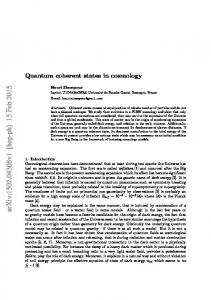


![Coherent Quantum LQG Control arXiv:0711.2551v2 [quant-ph] 24 May ...](https://m.moam.info/img/260x300/coherent-quantum-lqg-control-arxiv07112551v2-quant_5bb31068097c47f4428b4628.jpg)


