Optimizing Symbolic Model Checking for Constraint-Rich ... - CiteSeerX

Optimizing Symbolic Model Checking for Constraint-Rich Models Bwolen Yang

Reid Simmons Randal E. Bryant David R. O’Hallaron March 1999 CMU-CS-99-118

School of Computer Science Carnegie Mellon University Pittsburgh, PA 15213

A condensed version of this technical report will appear in Proceedings of the International Conference on Computer-Aided Verification, Trento, Italy (July 1999).

Effort sponsored in part by the Advanced Research Projects Agency and Rome Laboratory, Air Force Materiel Command, USAF, under agreement number F30602-96-1-0287, in part by the National Science Foundation under Grant CMS-9318163, and in part by grants from the Intel Corporation and NASA Ames Research Center. The U.S. Government is authorized to reproduce and distribute reprints for Governmental purposes notwithstanding any copyright annotation thereon. The views and conclusions contained herein are those of the author and should not be interpreted as necessarily representing the official policies or endorsements, either expressed or implied, of the Advanced Research Projects Agency, Rome Laboratory, or the U.S. Government.

Keywords: symbolic model checking, Binary Decision Diagram (BDD), timeinvariant constraints, redundant state-variable elimination, macro.

Abstract This paper presents optimizations for verifying systems with complex timeinvariant constraints. These constraints arise naturally from modeling physical systems, e.g., in establishing the relationship between different components in a system. To verify constraint-rich systems, we propose two new optimizations. The first optimization is a simple, yet powerful, extension of the conjunctivepartitioning algorithm. The second is a collection of BDD-based macro-extraction and macro-expansion algorithms to remove state variables. We show that these two optimizations are essential in verifying constraint-rich problems; in particular, this work has enabled the verification of fault diagnosis models of the Nomad robot (an Antarctic meteorite explorer) and of the NASA Deep Space One spacecraft.

1 Introduction This paper presents techniques for using symbolic model checking to automatically verify a class of real-world applications that have many time-invariant constraints. An example of constraint-rich systems is the symbolic models developed by NASA for on-line fault diagnosis [16]. These models describe the operation of components in complex electro-mechanical systems, such as autonomous spacecraft or robot explorers. The models consist of interconnected components (e.g., thrusters, sensors, motors, computers, and valves) and describe how the mode of each component changes over time. Based on these models, the Livingstone diagnostic engine [16] monitors sensor values and detects, diagnoses, and tries to recover from inconsistencies between the observed sensor values and the predicted modes of the components. The relationships between the modes and sensor values are encoded using symbolic constraints. Constraints between state variables are also used to encode interconnections between components. We have developed an automatic translator from such fault models to SMV (Symbolic Model Verifier) [11], where mode transitions are encoded as transition relations and state-variable constraints are translated into sets of time-invariant constraints. To verify constraint-rich systems, we introduce two new optimizations. The first optimization is a simple extension of the conjunctive-partitioning algorithm. The other is a collection of BDD-based macro-extraction and macro-expansion algorithms to remove redundant state variables. We show that these two optimizations are essential in verifying constraint-rich problems. In particular, these optimizations have enabled the verification of fault diagnosis models for the Nomad robot (an Antarctic meteorite explorer) [1] and the NASA Deep Space One (DS1) spacecraft [2]. These models can be quite large, with up to 1200 state bits. The rest of this paper is organized as follows. We first briefly describe symbolic model checking and how time-invariant constraints arise naturally from modeling (Section 2). We then present our new optimizations: an extension to conjunctive partitioning (Section 3), and BDD-based algorithms for eliminating redundant state variables (Section 4). We then show the results of a performance evaluation on the effects of each optimization (Section 5). Finally, we present a comparison to prior work (Section 6) and some concluding remarks (Section 7).

2 Background Symbolic model checking [5, 7, 11] is a fully automatic verification paradigm that checks temporal properties (e.g., safety, liveness, fairness, etc.) of finite state systems by symbolic state traversal. The core enabling technology for symbolic model checking is the use of the Binary Decision Diagram (BDD) representation [4] for 1

state sets and state transitions. BDDs represent Boolean formulas canonically as directed acyclic graphs such that equivalent sub-formulas are uniquely represented as a single subgraph. This uniqueness property makes BDDs compact and enables dynamic programming to be used for computing Boolean operations symbolically. To use BDDs in model checking, we need to map sets of states, state transitions, and state traversal to the Boolean domain. In this section, we briefly describe this mapping and motivate how time-invariant constraints arise. We finish with definitions of some additional terminology to be used in the rest of the paper.

2.1 Representing State Sets and Transitions In the symbolic model checking of finite state systems, a state typically describes the values of many components (e.g., latches in digital circuits) and each component is represented by a state variable. Let V = fv1 ; :::; vng be the set of state variables in a system, then a state can be described by assigning values to all the variables in V . This valuation can in term be written as a Boolean formula that is V true exactly for the valuation as ni=0 (vi == ci), where ci is the value assigned to the variable vi , and the “==” represents the equality operator in a predicate (similar to the C programming language). A set of states can be represented as a disjunction of the Boolean formulas that represent the states. We denote the BDD representation for a set of states S by S (V ). In addition to the set of states, we also need to map the system’s state transitions to the Boolean domain. We extend the above concept of representing a set of states to representing a set of ordered-pairs of states. To represent a pair of states, we need two sets of state variables: V the set of present-state variables for the first tuple and V 0 the set of next-state variables for the second tuple. Each variable v in V has a corresponding next-state variable v 0 in V 0 . A valuation of variables in V and V 0 can be viewed as a state transition from one state to another. A transition relation can then be represented as a set of these valuations. We denote the BDD representation of a transition relation T as T (V; V 0 ). In modeling finite state systems, the overall state transitions are generally specified by defining the valid transitions for each state variable. To support nondeterministic transitions of a state variable, the expression that defines the transitions evaluates to a set, and the next-state value of the state variable is nondeterministically chosen from the elements in the set. Hereafter, we refer to an expression that evaluates to a set either as a set expression or as a non-deterministic expression depending on the context, and we use the bold font type, as in f, to represent such expression. Let fi be the set expression representing state transitions of the state variable vi . Then the BDD representation for vi ’s transition relation Ti

2

can be defined as

Ti(V; V 0) := (vi0 2 fi (V )):

For synchronous systems, the BDD for the overall state transition relation T is

T (V; V 0) :=

n ^

i=0

Ti (V; V 0 ):

Detailed descriptions on this formulation, including mapping of asynchronous systems, can be found in [5, 11]. Note that in the above formulation, we also need to represent non-Boolean expressions (such as fi ’s) or non-Boolean variables as part of intermediate step. These non-Boolean formulas can be represented using variants of BDDs (e.g., MTBDD [6]) that extend the BDD concept to include non-Boolean values. These extensions also include algorithms for Boolean operators with non-Boolean arguments like the “==” and “2”. We will refer to all these BDD-variants simply as BDDs.

2.2 Time-Invariant Constraints and Their Common Usages In symbolic model checking, time-invariant constraints specify the conditions that must always hold. More formally, let C1, . . . , Cl be the time-invariant constraints and let C := C1 ^ C2 ^ ::: ^ Cl . Then, in symbolic state traversal, we consider only states where C is true. We refer to C as the constrained space. To motivate how time-invariant constraints arise naturally in modeling complex systems, we describe three common usages. One common usage is to make the same non-deterministic choice across multiple expressions in transition relations. For example, in a master-slave model, the master can non-deterministically choose which set of idle slaves to assign the pending jobs, and the slaves’ next-state values will depend on the choice made. To model this, let f be the non-deterministic expression representing how the master makes its choice. If the slaves’ transition relations are defined using the expression f directly, then each use of f makes its own non-deterministic choice independent of other uses. Thus, to ensure that all the slaves see the same non-deterministic choice, a new state variable u is introduced to record the choice made, and u is then used to define the slaves’ transition relations. This recording process is expressed as the time-invariant constraint u 2 f. Another common usage is for establishing the interface between different components in a system. For example, suppose two components are connected with a pipe of a fixed capacity. Then, the input of one component is the minimum of the pipe’s capacity and the output of the other component. This relationship is described as a time-invariant constraint between the input and the output of these two components. 3

Third common usage is specific uses of generic parts. For example, a bidirectional fuel pipe may be used to connect two components. If we want to make sure the fuel flows only one way, we need to constrain the valves in the fuel pipe. These constraints are specified as time-invariant constraints. In general, specific uses of generic parts arise naturally in both the software and the hardware domain as we often use generic building blocks in constructing a complex system. In the examples above, the use of time-invariant constraints is not always necessary because some these constraints can be directly expressed as a part of the transition relation and the associated state variables can be removed. However, these constraints are used to facilitate the description of the system or to reflect the way complex systems are built. Without these constraints, multiple expressions will need to be combined into possibly a very complicated expression. Performing this transformation manually can be labor intensive and error-prone. Thus it is up to the verification tool to automatically perform these transformations and remove unnecessary state variables. Our optimizations for constraint-rich models is to automatically eliminate redundant state variables (Section 4) and partition the remaining constraints (Section 3).

2.3 Symbolic State Traversal To reason about temporal properties, the pre-image and the image of the transition relation are used for symbolic state traversal, and time-invariant constraints are used to restrict the valid state space. Based on the BDD representations of a state set S and the transition relation T , we can compute the pre-image and the image of S , while restricting the computations to the constrained space C , as follows: pre-image(S )(V )

image(S )(V 0 )

:= :=

C (V ) ^ 9V 0 :[T (V; V 0) ^ (S (V 0 ) ^ C (V 0))] C (V 0 ) ^ 9V:[T (V; V 0 ) ^ (S (V ) ^ C (V ))]

(1) (2)

One limitation of the BDD representation is that the monolithic BDD for the transition relation T is often too large to build. A solution to this problem is the conjunctive partitioning [5] of the transition relation. In conjunctive partitioning, the transition relation is represented as a conjunction P1 ^ P2 ^ ::: ^ Pk with each conjunct Pi represented by a BDD. Then, the pre-image can be computed by conjuncting with one Pi at a time, and by using early quantification to quantify out variables as soon as possible. The early-quantification optimization is based on the property that sub-formulas can be moved out of the scope of an existential quantification if they do not depend on any of the variables being quantified. Formally, let Vi0 , a subset of V 0, be the set of variables that do not appear in any of the subsequent Pj ’s, where 1  i  k and i < j  k. Then the pre-image can be computed 4

as

p1 p2 pk pre-image(S )(V )

:= :=

.. . := :=

9V10 :[P1(V; V 0) ^ (S (V 0 ) ^ C (V 0))] 9V20 :[P2(V; V 0) ^ p1 ]

(3)

9Vk0 :[Pk (V; V 0 ) ^ pk?1 ]

C (V ) ^ pk

The determination and ordering of partitions (the Pi ’s in above) can have significant performance impact. Commonly used heuristics [8, 12] treat the state variables’ transition relations (Ti ’s) as the partitions. The ordering step then greedily schedules the partitions to quantify out more variables as soon as possible, while introducing fewer new variables. Finally, the ordered partitions are tentatively merged with their predecessors to reduce the number of intermediate results. Each merged result is kept only if the resulting graph size is less than a pre-determined limit. The conjunctive partitioning for the image computation is performed similarly with present-state variables in V being the quantifying variables instead of nextstate variables in V 0 . However, since the quantifying variables are different between the image and the pre-image computation, the resulting conjuncts for image computation is typically very different from those for pre-image computation.

2.4 Additional Terminology We define the support variables of a function to be the variables that the function depends on, and the support of a function to be the set of support variables. We define the ITE operator (if-then-else) as follows: given arbitrary expressions f and g where f and g may both be set expressions, and Boolean expression p, then ITE (p; f; g )(X ) :=



f (X ) g(X )

if p(X ); otherwise;

where X is the set of variables used in expressions p, f , and g . We define a carespace optimization as any algorithm care-opt that has following properties: given an arbitrary expression f where f may be a set expression, and a Boolean formula c, then care-opt(f; c) := ITE(c; f; d);

where d is defined by the particular algorithm used. The usual interpretation of this is that we only care about the values of f when c is true. We will refer to c as the 5

care space and :c as the don’t-care space. The goal of care-space optimizations is to heuristically minimize the representation for f by choosing a suitable d in the don’t-care space. Descriptions and a study of some care-space optimizations, including the commonly used restrict algorithm [7], can be found in [14].

3 Extended Conjunctive Partitioning The first optimization is the application of the conjunctive-partitioning algorithm on the time-invariant constraints. This extension is derived based on two observations. First, as with the transition relations, the BDD representation for timeinvariant constraints can be too large to be represented as a monolithic graph. Thus, it is crucial to represent the constraints as a set of conjuncts rather than a monolithic graph. Second, in constraint-rich models, many quantifying variables (variables being quantified) do not appear in the transition relation. There are two common causes for this. First, when time-invariant constraints are used to make the same non-deterministic choices, new variables are introduced to record these choices (described as the first example in Section 2.2). In the transition relation, these new variables are used only in their present-state form. Thus, their corresponding next-state variables do not appear in the transition relation, and for the pre-image computation, these next-state variables are parts of the quantifying variables. The other cause is that many state variables are used only to establish time-invariant constraints. Thus, both the present- and the next-state version of these variables do not appear in the transition relations. Based on this observation, we can improve the early-quantification optimization by pulling out the quantifying variables (V00 ) that do not appear in any of the transition relations. Then, these quantifying variables (V00 ) can be used for early quantification in conjunctive partitioning of the constrained space (C ) where the time-invariant constraints hold. Formally, let Q1 ; Q2; :::; Qm be the partitions produced by the conjunctive partitioning of the constrained space C , where C = Q1 ^ Q2 ^ ::: ^ Qm. For the pre-image computation, Equation 3 is replaced by

q1 q2 qm p1

:= :=

.. . := :=

9W10 :[Q1(V 0 ) ^ S (V 0)] 9W20 :[Q2(V 0 ) ^ q1 ]

0 :[Qm (V 0 ) ^ qm?1 ] 9Wm 9V10:[P1 (V; V 0 ) ^ qm ] 6

where Wi0 , a subset of V00 , is the set of variables that do not appear in any of the subsequent Qj ’s, where 1  i  m and i < j  m. Similarly, this extension also applies to the image computation.

4 Elimination of Redundant State Variables Our second optimization for constraint-rich models is targeted at reducing the state space by removing unnecessary state variables. This optimization is a set of BDDbased algorithms that compute an equivalent expression for each variable used in the time-invariant constraints (macro extraction) and then globally replace a suitable subset of variables with their equivalent expressions (macro expansion) to reduce the total number of variables. The use of macros is traditionally supported by language constructs (e.g., DEFINE in the SMV language [11]) and by simple syntactic analyses such as detecting deterministic assignments (e.g., a == f where a is a state variable and f is an expression) in the specifications. However, in constraint-rich models, the constraints are often specified in a more complex manner such as conditional dependencies on other state variables (e.g., p ) (a == f ) as conditional assignment of expression f to variable a when p is true). To identify the set of valid macros in such models, we need to combine the effects of multiple constraints. One drawback of syntactic analysis is that, for each type of expression, syntactic analysis will need to add a template to pattern match these expressions. Another more severe drawback is that it is difficult for syntactic analysis to estimate the actual cost of instantiating a macro. Estimating this cost is important because reducing the number of variables by macro expansion can sometimes result in significant performance degradation caused by large increases in other BDD sizes. These two drawbacks make the syntactic approach unsuitable for models with complex time-invariant constraints. Our approach uses BDD-based algorithms to analyze time-invariant constraints and to derive the set of possible macros. The core algorithm is a new assignmentextraction algorithm that extracts assignments from arbitrary Boolean expressions (Section 4.1). For each variable, by extracting its assignment form, we can determine the variable’s corresponding equivalent expression, and when appropriate, globally replace the variable with its equivalent expression (Section 4.2). The strength of this algorithm is that by using BDDs, the cost of macro expansion can be better characterized because the actual model checking computation is performed using BDDs. Note that there have been a number of research efforts on BDD-based redundant state-variable removal. To better compare our approach to these previous research efforts, we postpone the discussion of this prior work until Section 6, after

7

describing our algorithms and the performance evaluation.

4.1 BDD-Based Assignment Extraction The assignment-extraction problem can be stated as follows: given an arbitrary Boolean formula f and a variable v (where v can be non-Boolean), find g and h such that



f = (v 2 g) ^ h,

 g does not depend on v , and

h is a Boolean formula and does not depend on v. The expression (v 2 g) represents a non-deterministic assignment to variable v . In the case that g always evaluates to a singleton set, the assignment (v 2 g) is 

deterministic. A solution to this assignment-extraction problem is as follows:

h

=

t

=

g

=

9v:f

[

k2Kv

ITE(f jv k ; fkg; ;)

restrict(t; h)

where Kv is the set of all possible values of variable v , and restrict [7] is a carespace optimization algorithm that tries to reduce the BDD graph size (of t) by S collapsing the don’t-care space (:h). The BDD algorithm for the k2Kv operator is similar to the BDD algorithm for the existential quantification with the _ operator replaced by the [ operator for variable quantification. A correctness proof of this algorithm is included in Appendix A. Currently, we do not have any optimality guarantees for this solution. We do know that the solution g does not always have the minimum number of support variables. i.e., g is not necessary a minimum-support solution. However, based on the behavior of the restrict algorithm, we have formed a conjecture about the relationship between g and any minimum-support solution. Informally, this conjecture states that g can be converted to any minimum-support solution via a sequence of variable substitutions, and that these substitutions are parts of equality decomposition of h. More formally, Conjecture 1 Let gmin be a solution with the minimum number of support variei ) where ui ’s are ables. Then, there exists a sequence of n substitutions (ui variables, ei ’s are expressions, and 1  i  n, such that

 let g0

=

g, and gi

=

gi?1 jui ei for 1  i  n, then gn 8

=

gmin , and



h)(

Vn

i=1 (ui == ei )).

If this conjecture is true, then we know that even though each right-hand-side expression g extracted might have more support variables than necessary, these additional variables can be eliminated later by other macros (the (ui == ei )’s above). The above conjecture is based on the observation that given variable u, expressions f and e, where

f depends on u,  e does not depend on u, and  u’s variable order succeeds any of e’s support variables’ variable order, then, restrict (f; (u == e)) = f ju e . Another way of looking at this is that using restrict, a variable (u) might not be removed if its variable order does not come after the orders of its equivalent expression’s ( e’s) support variables. To prove the 

above conjecture, we will need to first prove that equality expressions are the only reason that the restrict algorithm may not produce minimum support solution. Note that in the assignment-extraction algorithm, the use of the restrict algorithm is not necessary. In fact, any care-space optimization algorithms can be used instead of the restrict algorithm. We choose to use the restrict algorithm because of the above property and because it works well in practice for other symbolicmodel-checking computations.

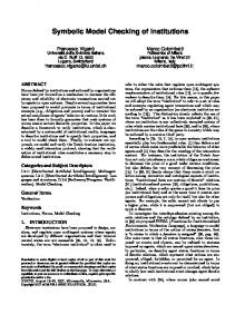
4.2 Macro Extraction and Expansion In this section, we describe the elimination of state variables based on macro extraction and macro expansion. The first step is to extract macros with the algorithm shown in Figure 1. This algorithm extracts macros from the constrained space (C ), which is represented as a set of conjuncts. It first uses the assignment-extraction algorithm to extract assignment expressions (line 5). It then identifies the deterministic assignments as candidate macros (line 6). For each candidate, the algorithm tests to see if applying the macro may be beneficial (line 7). This test is based on the heuristic that if the BDD graph size of a macro is not too large and its instantiation does not cause excessive increase in other BDDs’ graph sizes, then instantiating this macro may be beneficial. If the resulting right-hand-side g is not a singleton set, it is kept separately (line 9). These g’s are combined later (line 10) to determine if their intersection would result in a macro (lines 11-13). Finally, this algorithm returns the set of selected macros (line 14). After the macros are extracted, the next step is to determine the instantiation order. The main purpose of this algorithm (in Figure 2) is to remove circular dependencies. For example, if one macro defines variable v1 to be (v2 ^ v3) and a second 9

extract macros(C , V ) /* Extract macros for variables in V from the set C of conjuncts representing the constrained space */ 1 M /* initialize the set of macros found so far */ 2 for each v V 3 N /* initialize the set of non-singletons found so far */ 4 for each f C such that f depends on v 5 (g; h) assignment-extraction (f; v) /* f = (v g) h */ 6 if (g always returns a singleton set) /* macro found */ 7 if (is-this-result-good(g)) 8 M (v; g) M 9 else N g N 10 g’ g2N g 11 if (g’ always returns a singleton set) /* macro found */ 12 if ((is-this-result-good(g’)) 13 M (v; g’) M 14 return M

;

;

2

2

2 ^

f g[ f g[ T f

g[

Figure 1: Macro-extraction algorithm. In lines 7 and 12, “is-this-result-good” uses BDD properties (such as graph sizes) to determine if the result should be kept. macro defines v2 to be (v1 _ v4), then instantiating the first macro results in a circular definition in the second macro (v2 = (v2 ^ v3 ) _ v4 ) and thus invalidates this second macro. Similarly, the reverse is also true. To determine the set of macros to remove, the algorithm builds a dependence graph (line 1) and breaks circular dependencies based on graph sizes (lines 2-4). It then determines the ordering of the remaining macros based on the topological order (line 4) of the dependence graph. Finally, in the topological order, each macro (v; g) is instantiated in the remaining macros and in all other expressions (represented by BDDs) in the system, by substituting the variable v with its equivalent expression g.

5 Evaluation 5.1 Experimental Setup The benchmark suite used is a collection of 58 SMV models gathered from a wide variety of sources, including the 16 models used in a BDD performance study [17]. Out of these 58 models, 37 models have no time-invariant constraints, and thus our optimizations are not triggered and have no influence on the overall verification time. Out of the remaining 21 models, 10 very small models (< 10 seconds) 10

1 2 3 4 5

order macros(M ) /* Determine the instantiation order of the macros in set M */ /* first build the dependence graph G = (M; E ) */ M; y = (vy ; gy ) M; gy depends on vx E = (x; y ) x = (vx ; gx ) /* then remove circular dependences */ while there are cycles in G, MC set of macros that are in some cycle remove the macro with largest BDD size in MC return a topological ordering of the remaining macros in G

f

2

j

2

g

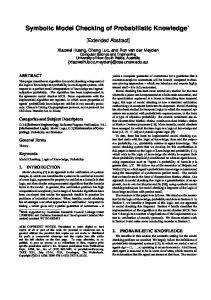
Figure 2: Macro-ordering algorithm. are eliminated. On the remaining 11 models, our optimizations have made nonnegligible performance impact on 7 models, where the results changed by more than 10 CPU seconds and 10% from the base case where no optimizations are enabled. In Figure 3, we briefly describe these 7 models. Note that some of these models are quite large, with up to 1200 state bits. Model acs ds1-b ds1 futurebus nomad v-gate xavier

# of State Bits 497 657 657 174 1273 86 100

Description the altitude-control module of NASA’s DS1 spacecraft a buggy fault diagnosis model for NASA’s DS1 spacecraft corrected version of ds1-b FutureBus cache coherency protocol fault diagnosis model for an Antarctic meteorite explorer reactor-system model fault diagnosis model for the Xavier robot

Figure 3: Description of models whose performance results are affected by our optimizations. The results reported in this section are labeled with the following keys to indicate which optimizations are enabled: None: no optimizations. Quan: the “early quantification on the constrained space” optimization (Section 3). SynM: syntactic analysis for macro-extraction and macro-expansion. This algorithm pattern matches deterministic assignment expressions (v == f , where v is a state variable and f is an expression) as macros and expands these macros. 11

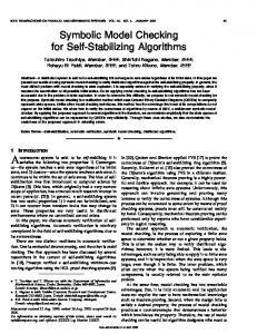
BDDM: the BDD-based macro extraction and macro expansion (Section 4). Q+SynM: both Quan and SynM optimizations. Q+BDDM: both Quan and BDDM optimizations. We performed the evaluation using the Symbolic Model Verifier (SMV) model checker [11] from Carnegie Mellon University. Conjunctive partitioning was used only when it was necessary to complete the verification. In these cases (including acs, nomad, ds1-b, and ds1), the size limit for each partition was set to 10,000 BDD nodes. For the remaining cases, the transition relations were represented as monolithic BDDs. The constrained space C was represented as a conjunction with each conjunct’s BDD graph size limited to 10,000 nodes. Without partitioning, we could not construct the BDD representation for the constrained space for 4 models. The evaluation was performed on a 200MHz Pentium-Pro with 1 GB of memory running Linux. Each run was limited to 6 hours of CPU time and 900 MB of memory. In Figure 4, we show the running time of different optimizations. Note that for all benchmarks, the time spent by our optimizations is very small (< 5 seconds or < 5% of total time) and is included in the running time shown. In the rest of this section, we analyze these results in the following order: the overall impact of our optimizations (Section 5.2), the impact of early quantification on the constraint space (Section 5.3), and the impact of macro optimization (Section 5.4). We then finish with a brief study on the impact of different size limits for conjunctive partitioning (Section 5.5). Model acs ds1-b ds1 futurebus nomad v-gates xavier

None (sec) m.o. m.o. m.o. 1410 m.o. 36 16

Quan (sec) 32 321 m.o. 53 t.o. 35 5

SynM (sec) m.o. t.o. m.o. 78 m.o. 51 6

BDDM (sec) 1059 m.o. t.o. 37 t.o. 50 5

Q+SynM (sec) 76 138 t.o. 35 7801 53 1

Q+BDDM (sec) 7 54 37 19 633 50 2

Figure 4: Running time with different optimizations enabled. The m.o.’s and t.o.’s are the results that exceeded the 900-MB memory limit and the 6-hour time limit, respectively.

12

5.2 Overall Results The results in Figure 5 show the overall performance impact of our optimizations. These results demonstrate that our optimizations have significantly improved the performance for 2 models (with speedups up to 74) and have enabled the verification of 4 models. For the v-gates model, the performance degradation (speedup = 0.7) is in the computation of the reachable states from the initial states. Upon further investigation, we believe that it is caused by the macro optimization, which increases the graph size of the transition relation from 122-thousand to 476-thousand nodes. This case demonstrates that reducing the number of state variables does not always improve performance. Model acs ds1-buggy ds1 futurebus nomad valves-gates xavier

None (sec) m.o. m.o. m.o. 1410 m.o. 36 16

Q+BDDM (sec) 7 54 367 19 633 50 2

None / Q+BDDM (speedup) enabled enabled enabled 74.2 enabled 0.7 8.0

Figure 5: Overall impact of our optimizations. The m.o.’s are the results that exceeded the 900-MB memory limit.

5.3 Impact of Early Quantification The results in Figure 6 show the impact of applying early quantification on timeinvariant constraints. The impact is measured both in the number of quantifying BDD variables extracted from the transition relations and in the performance speedups. The speedup results for None / Quan show that adding this optimization has enabled the verification of acs and ds1-b, and achieved significant performance improvement on futurebus (speedup of 26). The results in the Quan columns show that this improvement is mostly due to the fact that a large number of variables can be pulled out of the transition relations and applied to conjunctive partitioning and early quantification of the time-invariant constraints. From the Q+BDDM and BDDM / Q+BDDM columns, we observe similar results in presence of BDD-based macro optimization. Note that for the Q+BDDM columns, the “# of BDD vars extracted” results also include the number of BDD variables that are removed by the macro optimization. This is done to make the comparison between Quan and Q+BDDM results easier. 13

The results in Figure 6 show two additional interesting points. First, the number of variables extracted for pre-image computation is more than that extracted for image computation. This is because some variables are only used in their presentstate form in the transition relation (see first example in Section 2.2). Second, comparing the results between Quan and Q+BDDM columns indicates that the macro optimization generally does not interfere with the early-quantification optimization. The one exception is the nomad model, where the macro optimization introduced 114 BDD variables ((1121 - 1067) present-state variables plus (1174 1114) next-state variables) to the overall transition relation.

Model acs ds1-b ds1 futurebus nomad v-gates xavier

Total # of BDD Vars 994 1314 1314 348 2546 172 200

Effects of CP Optimization # of BDD vars extracted performance speedup Quan Q+BDDM None / BDDM / img p-img img p-img Quan Q+BDDM 439 449 437 449 enabled 151.0 550 566 546 566 enabled enabled 550 566 546 566 n/a enabled 58 110 54 110 26.6 1.9 1121 1174 1067 1114 n/a enabled 0 17 8 17 1.0 1.0 69 86 69 86 3.2 2.5

Figure 6: Effectiveness of the extended conjunctive-partitioning optimization. The effectiveness measures are (1) the number of quantifying BDD variables that are pulled out of the transition relation for early quantification of the time-invariant constraints, and (2) the impact on overall running time as performance speedups. For both measures, we present results both with (+BDDM) and without the BDDbased macro optimization. The n/a indicates that the speedup can not be computed because both cases failed to finish within the resource limits. Note: the number of BDD variables is twice the number of state variables—one copy for the present state and one copy for the next state.

5.4 Impact of Macro Extraction and Macro Expansion The results in Figure 7 show the impact of the BDD-based macro optimization, This impact is measured both in the number of BDD variables removed and in the performance speedups. The performance results in the None / BDDM column show that adding this optimization has enabled the verification of acs and achieved significant performance improvement on futurebus (speedup of 38). The results are similar in presence of the early-quantification optimization (the Quan / Q+BDDM 14

column). The results for “# of BDD vars removed” show that these performance improvements are due to the effectiveness of BDD-based macro optimization in removing variables; in particular, over a third of variables are removed for 4 models.

Model acs ds1-b ds1 futurebus nomad v-gates xavier

Total # of BDD Variables 994 1314 1314 348 2546 172 200

Effects of BDD-based Macro Optimization # of BDD performance speedup variables None / Quan / removed BDDM Q+BDDM 352 enabled 4.5 492 n/a 5.9 496 n/a enabled 18 38.1 2.7 844 n/a enabled 16 0.7 0.7 116 3.2 2.5

Figure 7: Effectiveness of macro optimizations. The effectiveness measures are (1) the number of BDD variables removed by macro optimization, and (2) the impact on overall running time as performance speedups. For both measures, we present results both with and without the early-quantification optimization. The n/a indicates that the speedup can not be computed because both cases failed to finish within the resource limits. Note: the number of BDD variables is twice the number of state variables. To evaluate the effectiveness of syntactic-based vs. BDD-based macro extraction, we compare the impact of these two approaches using both the number of BDD variables removed and the running time (Figure 8). The comparison is done for both with and without the early-quantification optimization. Note that the earlyquantification optimization does not affect the number of BDD variables removed. Thus, the “# of BDD vars removed” results are the same for both with and without the early-quantification optimization. Without the early-quantification optimization (the SynM / BDDM column), the results show that the BDD-based approach is better with the verification of acs enabled. With the early-quantification optimization (the Q+SynM / Q+BDDM column), the results show that the BDD-based approach has enabled the verification of ds1 and generally has better performance, with speedups of over 10 in acs and nomad. In the xavier case, the slowdown is 2 (speedup of 0.5) because the Q+BDDM used one extra second in macro extraction. The overall performance improvements are due to that the BDD-based approach is more effective in reducing the number of variables (“# of BDD vars removed” columns). In particular, for the acs, nomad, ds1-b, and ds1 models, > 150 additional BDD variables (i.e., 15

> 75 state bits) are removed in comparison to using syntactic analysis.

Model acs ds1-b ds1 futurebus nomad v-gates xavier

Total # of BDD Vars 994 1314 1314 348 2546 172 200

Syntax vs. BDD-based Macro Optimization # of BDD vars removed performance speedup SynM or BDDM or SynM / Q+SynM / Q+SynM Q+BDDM BDDM Q+BDDM 82 352 enabled 10.8 148 492 n/a 2.5 220 496 n/a enabled 12 18 2.1 1.8 688 844 n/a 12.3 16 16 1.0 1.0 64 116 1.2 1 / 2 = 0.5

Figure 8: Syntactic-based vs. BDD-based macro optimization. The effectiveness measures are (1) the number of BDD variables removed, and (2) the impact on overall running time as performance speedups. For both measures, we present results both with and without the early-quantification optimization. The n/a indicates that the speedup can not be computed because both cases failed to finish within the resource limits. Note: the number of BDD variables is twice the number of state variables.

5.5 Impact of Conjunctive-Partitioning Size Limit Because the conjunctive-partitioning algorithm often produces significantly different performance results with different partition-size limits, we have also reevaluated the above results using a partition-size limit of 100,000 nodes. The new results generally follow the same trend as before with the exception of ds1-b and ds1. For these two models, the results (Figure 9) show that if we choose the right partition-size limit for each case, we do not need to perform the macro optimization to verify them. (Note that this is not always true; e.g., the nomad model cannot be verified without the macro optimization.) However, with the BDD-based macro optimization (the Q+BDDM column), the performance results are more stable and are generally much better.

6 Related Work There have been many research efforts on BDD-based redundant state-variable removal in both logic synthesis and verification. These research efforts all use

16

Model ds1-b ds1-b ds1 ds1

Partition Size Limit (# of nodes) 10,000 100,000 10,000 100,000

None (sec) m.o. t.o. m.o. m.o.

Quan (sec) 321 309 m.o. 255

SynM (sec) t.o. t.o. m.o. t.o.

BDDM (sec) m.o. m.o. t.o. m.o.

Q+SynM (sec) 138 t.o. t.o. 92

Q+BDDM (sec) 54 101 37 74

Figure 9: Effects of the partition-size limit. The m.o.’s and t.o.’s are the results that exceeded the 900-MB memory limit and the 6-hour time limit, respectively. the reachable state space (set of states reachable from initial states) to determine functional dependencies for Boolean variables (macro extraction). The reachable state space effectively plays the same role as a time-invariant constraint, because the verification process only needs to check specifications in the reachable state space. Berthet et al. propose the first redundant state-variable removal algorithm in [3]. In [10], Lin and Newton describe a branch-and-bound algorithm to identify the maximum set of redundant state variables. In [13], Sentovich et al. propose new algorithms for latch removal and latch replacement in logic synthesis. There is also some work on detecting and removing redundant state variables while the reachable state space is being computed [9, 15]. From the algorithmic point of view, our approach is different from prior work in two ways. First, in determining the relationship between variables, the algorithms used to extract functional dependencies in previous work can be viewed as direct extraction of deterministic assignments to Boolean variables. In comparison, our assignment extraction algorithm is more general because it can also handle non-Boolean variables and extract non-deterministic assignments. Second, in performing the redundant state-variable removal, the approach used in the previous work would need to combine all the constraints first and then extract the macros directly from the combined result. However, for constraint-rich models, it may not be possible to combine all the constraints because the resulting BDD is too large to build. Our approach addresses this issue by first applying the assignment extraction algorithm to each constraint separately and then combining the results to determine if a macro can be extracted (see Figure 1). Another difference is that in previous work, the goal is to remove as many variables as possible. However, we have empirically observed that in some cases, removing additional variables can result in significant performance degradation in overall verification time (slowdown over 4). To address this issue, we use simple

17

heuristics (size of the macro and the growth in graph sizes) to choose the set of macros to expand. This simple heuristic works well in the test cases we tried. However, in order to fully evaluate the impact of different heuristics, we need to gather a larger set of constraint-rich models from a wider range of applications.

7 Conclusions and Future Work The two optimizations we proposed are crucial in verifying this new class of constraintrich applications. In particular, they have enabled the verification of real-world applications such as the Nomad robot and the NASA Deep Space One spacecraft. We have shown that the BDD-based assignment-extraction algorithm is effective in identifying macros. We plan to use this algorithm to perform a more precise cone-of-influence analysis with the assignment expressions providing the exact dependence information between the variables. In general, we plan to study how BDDs can be use to further help other compile-time optimizations in symbolic model checking.

Acknowledgement We thank Ken McMillan for discussions on the effects of macro expansion. We thank Olivier Coudert, Fabio Somenzi and reviewers for comments on this work. We are grateful to Intel Corporation for donating the machines used in this work.

A Correctness Proof for Assignment-Extraction Algorithm In this section, we present a correctness proof for the assignment-extraction algorithm in Section 4.1. Before presenting the main result, we first state and prove two supporting lemmas. Lemma 1 Let care-opt be any care-space optimization. Then, for arbitrary set expression t, Boolean formula h, and variable v ,

v 2 care-opt(t; h)) ^ h = care-opt(v 2 t; h) ^ h:

(

Proof By the definition of the care-space optimization, we have the following properties:

h h

) )

; h) == t); [care-opt(v 2 t; h) == (v 2 t)]: (care-opt(t

18

Therefore,

v 2 care-opt(t; h)) ^ h

(

v 2 t) ^ h care-opt(v 2 t; h) ^ h:

=

(

=

2 Lemma 2 Given an arbitrary Boolean formula f and a variable v . Let t=

[

ITE(f jv k ; fkg; ;);

k2Kv

where Kv is the set of all possible values of variable v . Then,

v 2 t) = f:

(

Proof

v2t

=

_

k0 ) ^ (k0 2 t) k 2K _ 0 0 [ ITE(f jv k ; fkg; ;)] (v == k ) ^ [k 2 k 2K k2K _ _ 0 0 (v == k ) ^ [k 2 ITE(f jv k ; fkg; ;)] k 2K k2K _ _ 0 ITE(f jv k ; k0 2 fkg; k0 2 ;) (v == k ) ^ k 2K k2K _ _ 0 ITE(f jv k ; k0 2 fkg; 0) (v == k ) ^ k 2K k2K _ 0 0 0 (v == k ) ^ ITE(f jv k ; k 2 fk g; 0) k 2K _ 0 (v == k ) ^ ITE(f jv k ; 1; 0) k 2K _ 0 (v == k ) ^ f jv k 0

=

0

=

0

=

0

=

0

=

v

v

v

v

v

v

v

v

v

0

0

=

v

0

0

=

v

( ==

v

0

k 2Kv 0

=

f:

2 Using the two lemmas above, we can now prove the correctness of the assignmentextraction algorithm. 19

Theorem 1 Given an arbitrary Boolean formula f and a variable v . Let

h

=

t

=

g

=

9v:f;

[

k2Kv

ITE(f jv k ; fkg; ;);

care-opt(t; h);

where care-opt is any care-space optimization algorithm and care-opt(t; h) does not depend on any new variables (other than those already in t and h). Then, the following conditions are true.

f = (v 2 g) ^ h,

1.

2. g does not depend on v , and

h is a Boolean formula and does not depend on v .

3. Proof

To prove Condition 1, we apply both Lemma 1 and Lemma 2 in the following derivation:

v 2 g) ^ h

(

= = = = = =

v 2 care-opt(t; h)) ^ h care-opt(v 2 t; h) ^ h care-opt(f; h) ^ h f ^h f ^ 9v:f f

(

Condition 2 is true because t does not depend on v (by construction) and the care-opt algorithm does not introduce new variable dependencies (given). Condition 3 is true because f is a Boolean formula and h = 9v:f is a Boolean formula that does not depend on v .

2

References [1]

BAPNA , D., ROLLINS , E., M URPHY, J., AND M AIMONE , M. The Atacama Desert trek - outcomes. In Proceedings of the 1998 International Conference on Robotics and Automation (May 1998), pp. 597–604.

20

[2]

B ERNARD, D. E., D ORAIS , G. A., F RY, C., J R ., E. B. G., K ANEFSKY, B., K URIEN, J., M ILLAR , W., M USCETTOLA , N., NAYAK , P. P., PELL , B., R AJAN , K., ROUQUETT, N., S MITH, B., AND W ILLIAMS , B. Design of the remote agent experiment for spacecraft autonomy. In Proceedings of the 1998 IEEE Aerospace Conference (March 1998), pp. 259–281.

[3]

B ERTHET, C., C OUDERT, O., AND M ADRE, J. C. New ideas on symbolic manipulations of finite state machines. In 1990 IEEE Proceedings of the International Conference on Computer Design (September 1990), pp. 224– 227.

[4]

B RYANT, R. E. Graph-based algorithms for Boolean function manipulation. IEEE Transactions on Computers C-35, 8 (August 1986), 677–691.

[5]

B URCH , J. R., CLARKE, E. M., L ONG , D. E., MC M ILLAN , K. L., AND D ILL , D. L. Symbolic model checking for sequential circuit verification. IEEE Transactions on Computer-Aided Design of Integrated Circuits and Systems 13, 4 (April 1994), 401–424.

[6]

C LARKE, E. M., MC M ILLAN , K. L., ZHAO , X., F UJITA , M., AND YANG , J. C.-Y. Spectral transform for large Boolean functions with application to technology mapping. In Proceedings of the 30th ACM/IEEE Design Automation Conference (June 1993), pp. 54–60.

[7]

C OUDERT, O., AND M ADRE, J. C. A unified framework for the formal verification of circuits. In Proceedings of the International Conference on Computer-Aided Design (Feb 1990), pp. 126–129.

[8]

G EIST, D., AND B EER , I. Efficient model checking by automated ordering of transition relation partitions. In Proceedings of the Computer Aided Verification (June 1994), pp. 299–310.

[9]

H U , A. J., AND D ILL , D. L. Reducing BDD size by exploiting functional dependencies. In Proceedings of the 30th ACM/IEEE Design Automation Conference (June 1993), pp. 266–71.

[10] L IN , B., AND N EWTON , A. R. Exact redundant state registers removal based on binary decision diagrams. IFIP Transactions A, Computer Science and Technology A, 1 (August 1991), 277–86. [11] M C M ILLAN , K. L. Symbolic Model Checking. Kluwer Academic Publishers, 1993.

21

[12] R ANJAN , R. K., AZIZ , A., B RAYTON , R. K., PLESSIER , B., AND P IXLEY, C. Efficient BDD algorithms for FSM synthesis and verification. Presented in the IEEE/ACM International Workshop on Logic Synthesis, May 1995. [13] S ENTOVICH , E. M., AND H ORIA TOMA , G. B. Latch optimization in circuits generated from high-level descriptions. In Proceedings of the International Conference on Computer-Aided Design (November 1996), pp. 428–35. [14] S HIPLE, T. R., H OJATI , R., S ANGIOVANNI -V INCENTELLI , A. L., AND B RAYTON , R. K. Heuristic minimization of BDDs using don’t cares. In Proceedings of the 31st ACM/IEEE Design Automation Conference (June 1994), pp. 225–231. [15]

E IJK , C. A. J., AND J ESS , J. A. G. Exploiting functional dependencies in finite state machine verification. In Proceedings of European Design and Test Conference (March 1996), pp. 266–71. VAN

[16] W ILLIAMS, B. C., AND NAYAK , P. P. A model-based approach to reactive self-configuring systems. In Proceedings of the Thirteenth National Conference on Artificial Intelligence and the Eighth Innovative Applications of Artificial Intelligence Conference (August 1996), pp. 971–978. [17] YANG , B., BRYANT, R. E., O’H ALLARON , D. R., BIERE, A., C OUDERT, O., JANSSEN , G., R ANJAN , R. K., AND S OMENZI , F. A performance study of BDD-based model checking. In Proceedings of the Formal Methods on Computer-Aided Design (November 1998), pp. 255–289.

22