Optimizing The Quality of Bootstrap-based Prediction Intervals

1

Optimizing The Quality of Bootstrap-based Prediction Intervals Abbas Khosravi, Saeid Nahavandi, Doug Creighton, and Dipti Srinivasan

Abstract The bootstrap method is one of the most widely used methods in literature for construction of confidence and prediction intervals. This paper proposes a new method for improving the quality of bootstrap-based prediction intervals. The core of the proposed method is a prediction interval-based cost function, which is used for training neural networks. A simulated annealing method is applied for minimization of the cost function and neural network parameter adjustment. The developed neural networks are then used for estimation of the target variance. Through experiments and simulations it is shown that the proposed method can be used to construct better quality bootstrap-based prediction intervals. The optimized prediction intervals have narrower widths with a greater coverage probability compared to traditional bootstrap-based prediction intervals.

I. I NTRODUCTION The application of Neural Networks (NNs) has proliferated in the last two decades in a variety of fields, such as finance, manufacturing, transportation, and energy systems. The popularity of NN models for forecasting and prediction is due to their universal approximation and learning capabilities [1] [2]. NN models are often developed and used for point prediction and forecasting. However, it is very important to have a measure of the reliability and accuracy of results generated by NN models. Confidence Intervals (CIs) and Prediction Intervals (PIs) are measures providing additional information about uncertainties affecting point predictions and forecasts. A noisy measured output can be represented as, 𝑡𝑖 = 𝑦𝑖 + 𝜖𝑖

(1)

where 𝑡𝑖 and 𝑦𝑖 are the i-th measured target (output) and the true regression mean of the target. 𝜖𝑖 is also the noise (random variable) with a zero expectation. The measured output is shifted from the true regression mean by the noise term. If the output of a developed model is represented by 𝑦ˆ𝑖 , the prediction/forecasting error can be written as, 𝑡𝑖 − 𝑦ˆ𝑖 = (𝑦𝑖 − 𝑦ˆ𝑖 ) + 𝜖𝑖

(2)

CIs are developed for measuring the variance of the first term in the right hand side of (2). They quantify the uncertainty between the prediction, 𝑦ˆ𝑖 , and the true regression, 𝑦𝑖 . PIs are more generic and quantify the uncertainty associated with the difference between the measured value, 𝑡𝑖 , and the predicted value, 𝑦ˆ𝑖 . As PIs account for more uncertainties, they are wider than CIs. The variance coverage of PIs makes them more informative than CIs, and therefore more useful for analysis and decision-making. The two terms in (2) are statistically independent. Hence, the total variance associated to the model outcome (prediction/forecast error) can be expressed as, 𝜎𝑖2 = 𝜎𝑦2ˆ𝑖 + 𝜎𝜖ˆ2𝑖

(3)

The term 𝜎𝑦2ˆ𝑖 originates from model mis-specification and parameter estimation errors. 𝜎𝜖ˆ2𝑖 is also the measure of noise variance. PIs take into account both the uncertainty in model structure and noise in data. Upon proper estimation of these values, PIs can be constructed for the outcomes of NN models. Associated with all CIs and PIs is a prescribed probability called the confidence level ((1 − 𝛼)%). It refers to the expected probability that the real value is within the predicted interval. A variety of techniques have been proposed in literature for construction of PIs for NN predictions and forecasts. The delta technique, described in [3] [4], is based on nonlinear regression theories and constructs PIs for linearized NN models around the set of optimal parameters obtained using the training algorithm. Khosravi et al. [5] improved the quality of PIs constructed using the delta technique for the case of load forecasting problem. This was done by training models through minimization of a novel PI-based cost function, rather than prediction error-based cost functions. The Bayesian technique [1] [6] constructs PIs based on the Bayesian learning algorithm. Both delta and Bayesian methods require calculation of complex matrices, such as the Hessian and Jacobian, and therefore, are computationally expensive. The bootstrap method Abbas Khosravi, Saeid Nahavandi, and Doug Creighton are with Centre for Intelligent Systems Research (CISR) at Deakin University, Geelong, Vic, Australia (email: {abbas.khosravi, saeid.nahavandi douglas.creighton}@deakin.edu.au). Dr. Dipti Srinivasan is an associate professor with the Department of Electrical and Computer Engineering, National University of Singapore, 4 Engineering Drive 3, Singapore 117576 (email: dipti@[email protected]).

2

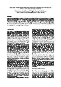
[7] [8] is a resampling method that uses 𝐵 + 1 NN models to predict the target and estimate the variance of the targets required for construction of PIs. The mean-variance estimation method [9] [10] uses two NNs for construction of PIs. The first NN is used for estimation of the true regression mean, and the second NN estimates the target variance. A very fast method for construction of reliable PIs was also proposed in [11]. The method uses a NN with two outputs for estimating lower and upper bounds of PIs. Application of these methods have been reported in fields such as transportation systems [12] [10] [13], energy systems [5] [14], temperature prediction [15], manufacturing systems [16], and power generation [17]. The focus of this paper is on the bootstrap technique for construction of PIs for outcomes of NN models. The research objective is to improve the quality of constructed PIs in terms of their width and coverage probability. In fact, this paper aims to make bootstrap-based PIs narrower than traditional PIs without compromising their coverage probability. This will be achieved through an innovative new model development technique applied to the NNs used for estimation of the target variance. Performance of the proposed method will be examined for different case studies. Quantitative measures will be used for assessing the quality of optimized bootstrap-based PIs. The rest of this paper is organized as follows. Section II describes the bootstrap method for construction of PIs. PI assessment measures and indices are briefly discussed in Section III. The proposed method for optimizing the quality of bootstrap-based PIs is discussed in Section IV. Simulation results are represented in Section V. Section VI concludes the paper with a conclusion and some remarks. II. B OOTSTRAP M ETHOD FOR PI C ONSTRUCTION Fusion of multiple estimators/models to improve the overall prediction performance is the key idea behind the bootstrap method. This is done to leverage the complementary predictive characteristics of models developed using different datasets. Diverse datasets for creation of different models can be generated using the bootstrap method. 𝐵 training datasets are resampled from the original dataset with replacement, 𝐷𝑏 , 𝑏 = 1, . . . , 𝐵. The method estimates the variance due to model mis-specification, 𝜎𝑦2ˆ, by building 𝐵 𝑁 𝑁𝑦 models (Fig. 1). The true regression is estimated by averaging the point forecasts of 𝐵 models, 𝑦ˆ𝑖 =

𝐵 1 ∑ 𝑏 𝑦ˆ𝑖 𝐵

(4)

𝑏=1

where 𝑦ˆ𝑖𝑏 is the prediction of the i-th sample generated by the b-th bootstrap model. Assuming that NN models are unbiased, the model mis-specification variance can be estimated using the variance of 𝐵 model outcomes, 𝐵

𝜎𝑦2ˆ𝑖 =

)2 1 ∑( 𝑏 𝑦ˆ𝑖 − 𝑦ˆ𝑖 𝐵−1

(5)

𝑏=1

This variance is mainly due to the random initialization of parameters and using different datasets for training NNs. To construct PIs, we also need to estimate the variance of errors, 𝜎𝜖ˆ2𝑖 . The key idea is to develop a separate individual NN model, called 𝑁 𝑁𝜎𝜖ˆ to provide an estimate of 𝜎𝜖ˆ2𝑖 when presented with an input vector. The transfer function of the output unit of 𝑁 𝑁𝜎𝜖ˆ is assumed to be exponential instead of a linear transfer function to ensure that the variance is always positive. From (3), 𝜎𝜖ˆ2 can be calculated as follow, 2

𝜎𝜖ˆ2 ≃ 𝐸{(𝑡 − 𝑦ˆ) } − 𝜎𝑦2ˆ

(6)

According to (6), a set of variance squared residuals is developed, ( ) 𝑟𝑖2 = 𝑚𝑎𝑥 (𝑡𝑖 − 𝑦ˆ𝑖 )2 − 𝜎𝑦2ˆ𝑖 , 0

(7)

where 𝑦ˆ𝑖 and 𝜎𝑦ˆ𝑖2 are obtained from (4) and (5). These residuals are linked by the set of corresponding inputs to form a new dataset, { }𝑛 𝐷𝑟2 = (𝑥𝑖 , 𝑟𝑖2 ) 𝑖=1

(8)

A new NN model can be indirectly trained to estimate the unknown values of 𝜎𝜖ˆ2𝑖 , so as to maximize the probability of observing samples in 𝐷𝑟2 . The model development can be done using the maximum likelihood as the cost function, ( ) 𝑛 2 𝑟 1∑ 𝑙𝑛(𝜎𝜖ˆ2𝑖 ) + 2𝑖 (9) 𝐶𝐵𝑆 = 2 𝑖=1 𝜎𝜖ˆ𝑖 Using this cost function, an indirect two phase training technique can be used [9] for adjusting parameters of bootstrap 1 2 NNs and 𝑁 𝑁𝜎𝜖ˆ . The algorithm needs two datasets, namely 𝐷𝑡𝑟𝑎𝑖𝑛 and 𝐷𝑡𝑟𝑎𝑖𝑛 , for training 𝐵 bootstrap NN models 𝑁 𝑁𝑦 and

3

NN1

yˆ 1 D1

yˆ

NN2

yˆ

D2

2

Dataset

 y2ˆ DB NNB

yˆ B

Fig. 1.

An ensemble of 𝐵 NN models used by the Bootstrap method.

𝑁 𝑁𝜎𝜖ˆ . In Phase I of the training algorithm, bootstrap NN models are trained to estimate 𝑡𝑖 . In Phase II, bootstrap NN models 2 are kept unchanged, and 𝐷𝑡𝑟𝑎𝑖𝑛 is used for adjusting parameters of 𝑁 𝑁𝜎𝜖ˆ . Adjusting of parameters of 𝑁 𝑁𝜎𝜖ˆ is achieved through minimizing the cost function defined in (9). Parameters of 𝑁 𝑁𝜎𝜖ˆ can be updated using the traditional gradient descent-based methods or stochastic-based optimization techniques, such as genetic algorithm or simulated annealing. Once both 𝜎𝑦ˆ𝑖2 and 𝜎𝜖ˆ2𝑖 are known, the i-th PI with a confidence level of (1 − 𝛼)% can be constructed, √ 1− 𝛼 (10) 𝑦ˆ𝑖 ± 𝑡𝑑𝑓 2 𝜎𝑦2ˆ𝑖 + 𝜎𝜖ˆ2𝑖 1− 𝛼

where 𝑡𝑑𝑓 2 is the 1 − 𝛼2 quantile of a cumulative t-distribution function with 𝑑𝑓 degrees of freedom. The described bootstrap method is traditionally called the bootstrap pairs. There exists another bootstrap method, called bootstrap residuals, which resamples the prediction residuals. Further information on this method can be found in [18]. III. PI A SSESSMENT Assessment of the quality PIs is done using three performance measures, PICP, NMPIW, and CWC, proposed in [5] [11] [19]. The most important characteristic of PIs is their coverage probability. PI Coverage Probability (PICP) is measured by counting the number of target values covered by the constructed PIs, 𝑛

𝑃 𝐼𝐶𝑃 =

1∑ 𝑐𝑖 𝑛 𝑖=1

(11)

where, 𝑐𝑖 =

⎧ ⎨1 𝑡𝑖 ∈ [𝐿𝑖 , 𝑈𝑖 ] ⎩

(12)

0 𝑡𝑖 ∈ / [𝐿𝑖 , 𝑈𝑖 ]

where 𝑛 is the number of samples, and 𝐿𝑖 and 𝑈𝑖 are lower and upper bounds of the i-th PI respectively. Ideally, PICP should be very close or larger than the nominal confidence level associated to the PIs. Although wide PIs have a satisfactory coverage probability greater than the nominal confidence level, they are less informative. Therefore, it is essential to assess PIs based on their width. Mean PI Width (MPIW) quantifies how wide constructed PIs are, 𝑛

𝑀 𝑃 𝐼𝑊 =

1∑ (𝑈𝑖 − 𝐿𝑖 ) 𝑛 𝑖=1

(13)

MPIW shows the average width of PIs. Normalizing MPIW by the range of the underlying target, 𝑅, allows us to compare PIs constructed for different datasets respectively. The new measure is called NMPIW, 𝑀 𝑃 𝐼𝑊 (14) 𝑅 Both PICP and NMPIW evaluate the quality of PIs from one aspect. The Coverage Width-based Criterion (CWC) simultaneously evaluates PIs from both coverage probability and width perspectives, 𝑁 𝑀 𝑃 𝐼𝑊 =

4

) ( 𝐶𝑊 𝐶 = 𝑁 𝑀 𝑃 𝐼𝑊 1 + 𝛾(𝑃 𝐼𝐶𝑃 ) 𝑒−𝜂(𝑃 𝐼𝐶𝑃 −𝜇)

(15)

where 𝛾(𝑃 𝐼𝐶𝑃 ) is given by, 𝛾(𝑃 𝐼𝐶𝑃 ) =

⎧ ⎨0 𝑃 𝐼𝐶𝑃 ≥ 𝜇 ⎩

(16)

1 𝑃 𝐼𝐶𝑃 < 𝜇

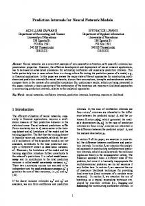
𝜂 and 𝜇 in (15) are two hyperparameters controlling the location and amount of CWC jump. The CWC provides an effective compromise between informativeness (being narrow) and correctness (having an acceptable coverage probability) of PIs. IV. P ROPOSED M ETHOD In the proposed method, 𝜎𝑦2ˆ𝑖 of the bootstrap method is estimated using (5). However, the procedure for construction of 𝑁 𝑁𝜎𝜖ˆ to estimation 𝜎𝜖ˆ2𝑖 is different. The key idea here is to train the 𝑁 𝑁𝜎𝜖ˆ through minimization of a PI-based cost function, rather than the one defined in (9). The ultimate purpose of NN development is construction of PIs. So, it is more reasonable to train NNs for improving the quality of constructed PIs. The CWC measure, as defined in (15) is considered as the cost function here for training of 𝑁 𝑁𝜎𝜖ˆ . As discussed, CWC covers two important properties of PIs: widths and coverage probability. It is expected that adjustment of parameters of 𝑁 𝑁𝜎𝜖ˆ through minimization of CWC will greatly improve the quality of PIs constructed using the bootstrap technique. Here, we use simulated annealing method for minimization of CWC as the cost function and for adjusting parameters of 𝑁 𝑁𝜎𝜖ˆ . Simulated Annealing (SA) [20] [21] is a Monte Carlo technique that can be used for seeking out the global minimum. Compared with traditional mathematical optimization techniques, SA offers a number of advantages, such as being derivative-free and less-likely to be trapped in local minima. In every iteration of SA, a new set of parameters is generated. The cost function is assessed for the new set of parameters. If the cost function has been decreased, the set of parameters are recorded as the best solution. Otherwise, the decision to accept or discard the current solution is made based on the Boltzman mechanism. The key parameter in this mechanism is the cooling temperature. When the cooling factor is large, uphill movements are accepted. As it is decreased by applying an exponential or geometric cooling schedule, optimization becomes greedy and only improving transitions are accepted. The procedure for construction of bootstrap-based PIs remains unchanged up to stage of training 𝑁 𝑁𝜎𝜖ˆ . 𝐵 NN models 1 are developed using 𝐵 datasets formed by resampling the original training dataset (𝐷𝑡𝑟𝑎𝑖𝑛 ). Then SA is applied for training 2 of 𝑁 𝑁𝜎𝜖ˆ using samples of 𝐷𝑡𝑟𝑎𝑖𝑛 . In each iteration, PIs are constructed using (10). 𝜎𝑦2ˆ𝑖 and 𝜎𝜖ˆ2𝑖 are obtained using (5) and 𝑁 𝑁𝜎𝜖ˆ . The quality of PIs is assessed using CWC. Optimization and adjustment of parameters of 𝑁 𝑁𝜎𝜖ˆ is continued until no progress is achieved in several iterations. An interesting feature of the proposed method is that no target is required for training of 𝑁 𝑁𝜎𝜖ˆ . What is important here is the quality of PIs measured by CWC. The parameters of 𝑁 𝑁𝜎𝜖ˆ are adjusted to result in the highest quality PIs, even if the values of 𝜎𝜖ˆ2𝑖 are unknown. Once the optimization is finished, 𝐵 + 1 NN models are used for construction of optimized PIs. V. S IMULATION R ESULTS The performance of the proposed method is examined using datasets taken from a real world baggage handling system. The targets are time required for processing 70% and 90% of each flight bags. Hereafter, we refer to these targets as T70 and T90. Fig. 2 shows these two targets (totally 272 samples). Travel times of bags fluctuate significantly for different flights and are highly affected by several uncontrollable events occurring during process of bags. Flight type (economy or economybusiness), check-in counter (six piers), exit lateral or makeup loop (totally 40), and work-in-progress are input variables for both 𝑁 𝑁𝑦 (B models) and 𝑁 𝑁𝜎𝜖ˆ . Datasets considered here have previously been used for benchmarking performance of other PI construction methods [11] [19]. Available samples are randomly split into three subsets: first and second training 1 2 sets (𝐷𝑡𝑟𝑎𝑖𝑛 and 𝐷𝑡𝑟𝑎𝑖𝑛 ) each accounts for 40% of samples (totally 80% for training). The test set (𝐷𝑡𝑒𝑠𝑡 ) consists of 20% of the samples. All variables are pre-processed to have zero mean and unit variance. This is done to give all input variables an equal chance for contribution to the model and avoid having models biased towards inputs with large values. Two layer NNs are considered for developing 𝐵 𝑁 𝑁𝑦 models and an individual 𝑁 𝑁𝜎𝜖ˆ model. Preliminary experiments are conducted for determining the optimal structure of the NNs and selecting the number of neurons in the hidden layers. Table I shows values for different parameters used by the NNs and the SA method. SA uses a geometric cooling schedule with a cooling factor of 0.9. All PIs are constructed with a confidence level set to 90%. Values for 𝜂 and 𝜇 are set to those recommended in [11]. Ten bootstrap NN models are considered for prediction of the i-th target and estimation of 𝜎𝑦2ˆ𝑖 in (5).

5

Fig. 2.

Plot of targets, (top) T70, and (bottom) T90. TABLE I PARAMETERS USED IN THE EXPERIMENTS BY NN S AND SA Parameter 1 𝐷𝑡𝑟𝑎𝑖𝑛 2 𝐷𝑡𝑟𝑎𝑖𝑛 𝐷𝑡𝑒𝑠𝑡 Structure of 𝑁 𝑁𝑦 Structure of 𝑁 𝑁𝜎𝜖ˆ Number of bootstrap models (B) 𝛼 𝜂 𝜇 𝜅 𝑇0 Geometric cooling schedule

Numerical Value 40% of all samples 40% of all samples 20% of all samples 4-8-4-1 4-6-4-1 10 0.1 50 0.90 1 5 𝑇𝑘+1 = 0.9 𝑇𝑘

NNs are unstable in terms of prediction results and their performance may change from one simulation to another due to effects of random initialization. Experiments with each target are repeated ten times and all results are reported to avoid any misleading judgment about performance of proposed method for construction of optimized bootstrap-based PIs. In each replicate, training and test datasets are randomly regenerated and used for construction of PIs. The convergence history of the training algorithm and minimization of the cost function is shown in Fig. 3 for T70, replicate 8. The cooling temperature is decreased from 5 to a small value close to zero. Uphill movements can be found till iteration 250. After this point, optimization becomes greedy and converges to the optimal solution. Optimization algorithm terminates after almost 550 iterations, which takes less than 10 seconds to be completed on a computer with an Intel 2.53GHz processor and 8GB RAM. Fig. 4 and Fig. 5 show CWC measures computed for PIs constructed for T70 and T90 using traditional and proposed bootstrap method. The quality of 𝑃 𝐼𝑛𝑒𝑤 is superior to the quality of 𝑃 𝐼𝑡𝑟𝑎𝑑 in 7 out of 10 replicates for both targets. For T70, the best improvement is achieved in replicate 8, where 𝐶𝑊 𝐶𝑇 70 is decreased from 94.2 to 62.9, more than a 33% improvement. The worst experiment for T70 is replicate 5. 𝐶𝑊 𝐶𝑇𝑛𝑒𝑤 70 is too large (more than 200). This might be caused by an early termination of the optimization algorithm resulting in an improper set of parameters for 𝑁 𝑁𝜎𝜖ˆ . For the case of T90, results are more consistent and there is no problem with early termination of the training algorithm. 𝑛𝑒𝑤 The maximum improvement is obtained in replicate 4, where 𝐶𝑊 𝐶𝑇𝑡𝑟𝑎𝑑 90 and 𝐶𝑊 𝐶𝑇 90 are 102.7 and 57.8 respectively (almost 57% improvement). With the exception of replicate 5 for T70, the average improvement in ten replicates for T70 and T90 are 11.2% and 9.8% respectively. These average results indicate that the proposed method for construction of optimized bootstrap PIs leads to better quality PIs. These intervals are narrower and their PICP is greater than the nominal confidence level (90%).

6

Fig. 3. 8.

The convergence behavior of the optimization algorithm (top) the cooling temperature, and (bottom) the cost function, visualized for T70, replicate

200

Traditional New

180.0

180 160

140.6

140

CWC

120

115.8

100

94.2

90.4

83.2

80

68.5

67.6

62.9

60.1

56.8

60

48.9

46.5

46.1

40

62.6 51.0

42.2

40.1

33.0

20 0 1

2

3

4

5

6

7

8

9

10

Replicate

Fig. 4.

CWC measure in ten replicates of experiments for traditional and proposed bootstrap-based PIs constructed for T70. 180.0

Traditional New

160.0 140.0

122.0 117.2

CWC

120.0 100.0

146.5

133.3

106.3 101.4

121.8

102.7 95.2

91.4

80.0

76.5 75.1 63.8 57.8

60.0

54.9

54.5

46.3

44.2

41.3

40.0

33.5

20.0 0.0 1

2

3

4

5

6

7

8

9

10

Replicate

Fig. 5.

CWC measure in ten replicates of experiments for traditional and proposed bootstrap-based PIs constructed for T90.

Fig. 6 displays T70 PIs constructed using proposed and traditional bootstrap method in the 8th replicate. A visual analysis 𝑡𝑟𝑎𝑑 and comparison makes clear that 𝑃 𝐼𝑇𝑛𝑒𝑤 70 are much narrower than 𝑃 𝐼𝑇 70 . Wide PIs are an indication of presence of a high level of uncertainty in data. These uncertainties make point prediction less reliable and ruin the generalization power of NN 𝑡𝑟𝑎𝑑 models. As 𝑃 𝐼𝑇𝑛𝑒𝑤 70 have a higher quality compared to 𝑃 𝐼𝑇 70 , we can conclude that the proposed method more efficiently handles effects of uncertainties on predicted values. This is a result of directly training NN models based on characteristics

7

Fig. 6.

PIs for T70 obtained in replicate 8 using (top) traditional bootstrap method, and (bottom) the proposed bootstrap method.

of PIs. Comparison of PIs in Fig. 6 reveals that 𝑃 𝐼𝑇 70 are wider than 𝑃 𝐼𝑇 90 . This is due to the fact that effects of uncertainties on 𝑃 𝐼𝑇 90 are significantly more than effects of uncertainties on 𝑃 𝐼𝑇 70 . More uncertainties are caused by occurrence of unpredictable events such as missing tags or bags uncleared by screening machines requiring further attention. As these greatly increase travel times of bags, the corresponding PIs constructed using the bootstrap method are wider. Performance of the proposed method in this paper for construction of PIs can be further improved. Here are some guidelines: ∙ In the conducted simulation here it has been assumed that the structure of NNs is a priori determined. Such an approach may lead to not globally optimal PIs, as NN structure has a significant effect on the generalization power and performance of NN models. The number of neurons in hidden layers of NNs can be integrated into the optimization problem as a key decision variable. The proposed PI-based cost function can be applied for determination of this new variable. ∙ Performance of NNs is highly susceptible to their initialization procedure. Performance of the proposed method can be further improved in case of using an appropriate initial set. An alternative is the set of parameters obtained from traditional bootstrap method. ∙ New PI-based cost functions can be developed and applied for training of NN models. The current PI-based cost function examines PIs based on their width and coverage probability. New cost functions can have a different penalization mechanism (rather than exponential) or use other features of PIs. ∙ Other optimization algorithm, such as genetic algorithm, can be applied for minimization of the cost function and adjustment of 𝑁 𝑁𝜎𝜖ˆ parameters. Continuing the optimization algorithm for more iterations (generations) can improve performance of the proposed method for PI construction. VI. C ONCLUSIONS A new method was proposed in this paper for optimal construction of prediction intervals using the bootstrap method. In the proposed method, neural networks for estimation of the target variance are trained using an innovative prediction intervalbased cost function. The cost function covers two important quality aspects of prediction intervals: width and coverage probability. A simulated annealing method was applied for minimization of the cost function and adjusting neural network parameters. Experiments conducted with real case studies revealed that application of the proposed method improves the quality of prediction intervals constructed using the bootstrap method by more than 10%. ACKNOWLEDGMENT This research was fully supported by the Centre for Intelligent Systems Research (CISR) at Deakin University.

8

R EFERENCES [1] C. M. Bishop, Neural Networks for Pattern Recognition. Oxford University, Press, Oxford, 1995. [2] K. Hornik, M. Stinchcombe, and H. White, “Multilayer feedforward networks are universal approximators,” Neural Networks, vol. 2, no. 5, pp. 359–366, 1989. [3] J. T. G. Hwang and A. A. Ding, “Prediction intervals for artificial neural networks,” Journal of the American Statistical Association, vol. 92, no. 438, pp. 748–757, 1997. [4] R. D. d. Veaux, J. Schumi, J. Schweinsberg, and L. H. Ungar, “Prediction intervals for neural networks via nonlinear regression,” Technometrics, vol. 40, no. 4, pp. 273–282, 1998. [5] A. Khosravi, S. Nahavandi, and D. Creighton, “Construction of optimal prediction intervals for load forecasting problem,” IEEE Transactions on Power Systems, vol. 25, pp. 1496–1503, 2010. [6] D. J. C. MacKay, “The evidence framework applied to classification networks,” Neural Computation, vol. 4, no. 5, pp. 720–736, 1992. [7] B. Efron, “Bootstrap methods: Another look at the jackknife,” The Annals of Statistics, vol. 7, no. 1, pp. 1–26, 1979. [8] T. Heskes, “Practical confidence and prediction intervals,” in Neural Information Processing Systems, T. P. M. Mozer, M. Jordan, Ed., vol. 9. MIT Press, 1997, pp. 176–182. [9] D. Nix and A. Weigend, “Estimating the mean and variance of the target probability distribution,” in IEEE International Conference on Neural Networks, 1994. [10] E. Mazloumi, G. Rose, G. Currie, and S. Moridpour, “Prediction intervals to account for uncertainties in neural network predictions: Methodology and application in bus travel time prediction,” Engineering Applications of Artificial Intelligence, vol. In Press, Corrected Proof, 2010. [11] A. Khosravi, S. Nahavandi, D. Creighton, and A. F. Atiya, “A lower upper bound estimation method for construction of neural network-based prediction intervals,” IEEE Transactions on Neural Networks, DOI: 10.1109/TNN.2010.2096824, Accepted on 28-Nov-2010. [12] A. Khosravi, E. MAzloumi, S. Nahavandi, D. Creighton, and J. W. C. van Lint, “Prediction intervals to account for uncertainties in travel time prediction,” IEEE Transactions on Intelligent Transportation Systems , DOI: 10.1109/TITS.2011.2106209, Available online: 04 February 2011. [13] C. van Hinsbergen, J. van Lint, and H. van Zuylen, “Bayesian committee of neural networks to predict travel times with confidence intervals,” Transportation Research Part C: Emerging Technologies, vol. 17, no. 5, pp. 498–509, Oct. 2009. [14] A. Khosravi, S. Nahavandi, and D. Creighton, “Load forecasting and neural networks: A prediction interval-based perspective,” B.K. Panigrahi et al. (Eds.): Computational Intelligence in Power Engineering, SCI 302, pp. 131–150, 2010. [15] T. Lu and M. Viljanen, “Prediction of indoor temperature and relative humidity using neural network models: model comparison,” Neural Computing & Applications, vol. 18, no. 4, pp. 345–357, May 2009. [16] G. Yu, H. Qiu, D. Djurdjanovic, and J. Lee, “Feature signature prediction of a boring process using neural network modeling with confidence bounds,” The International Journal of Advanced Manufacturing Technology, vol. 30, no. 7, pp. 614–621, Oct. 2006. [17] E. Zio, “A study of the bootstrap method for estimating the accuracy of artificial neural networks in predicting nuclear transient processes,” IEEE Transactions on Nuclear Science, vol. 53, no. 3, pp. 1460–1478, 2006. [18] R. Tibshirani, “A comparison of some error estimates for neural network models,” Neural Computation, vol. 8, pp. 152–163, 1996. [19] A. Khosravi, S. Nahavandi, and D. Creighton, “A prediction interval-based approach to determine optimal structures of neural network metamodels,” Expert Systems with Applications, vol. 37, pp. 2377–2387, 2010. [20] G. C. V. M. Kirkpatrick, S., “Optimization by simulated annealing,” Science, vol. 220, pp. 671–680, 1983. [21] E. H. L. Laarhoven, P. J. M. van Aarts, Simulated annealing : theory and applications. Dordrecht, Boston, Norwell, MA, U.S.A., Kluwer Academic Publishers, 1987.