F.G. Badía and M.D. Berrade / International Journal of Materials & Structural Reliability Vol.4, No.1, March 2006, 27-37
International Journal of Materials & Structural Reliability International Journal of Materials & Structural Reliability Vol.4, No.1, March 2006, 27-37
Optimum Maintenance of a System under two Types of Failure F.G. Badía* and M.D. Berrade Department of Statistics, C.P.S. University of Zaragoza, María de Luna 3, 50015 Zaragoza, Spain
Abstract A maintenance model for a system subject to both unrevealed catastrophic failures or revealed minor failures is presented. The former are detected by means of an inspection policy at periodic times kT, k=1,2,…. Moreover it is assumed a less than perfect testing, that is, false alarms as well as undetected failures after an inspection. Revealed failures are removed by a minimal repair whereas a perfect repair follows the unrevealed failures. A renewal of the system after the th
N revealed failure completes the maintenance actions. The times of inspections and repairs are also taken into account. The expected cost-minimizing policy along an infinite time span is also analyzed. Keyword: Maintenance, Minimal repair, Optimum policy, Reliability, Unrevealed failure
1. Introduction The design of maintenance policies turns out to be a crucial issue in reliability theory. Failures reduce the ability to fulfill specific functions and are often responsible for huge economic losses. The costs derived from defective production or downtime incurred when a system fails, lead those non-negligible money figures currently invested in maintenance procedures in order to prevent the systems to fail. The classical age replacement and block replacement policies [1] are specially designed for revealed failures, which are detected as soon as they occur. However many engineering systems are subject to the so-called unrevealed failures when inspections or special tests are needed to discover them. Failures of this sort occur in systems that alternate both operating and idle periods such as spares or units in stand-by mode. Security devices in gas conductions, nuclear power plants, or fire alarms are typical examples of systems which may undergo unrevealed failures [4, 10, 11, 12]. Thus, periodic inspection emerges due to the unaffordable cost of a continuous monitoring. The model in [2] considers cost optimization by selection of a unique interval for both inspection and maintenance. The model in [12] provides an imperfect inspection policy which have non-zero probability of false positives along with preventive actions for a system subject to three competing failure types. *
Corresponding author. E-mail :
[email protected]
27
F.G. Badía and M.D. Berrade / International Journal of Materials & Structural Reliability Vol.4, No.1, March 2006, 27-37
A maintenance policy that suits a system presenting two types of failure is presented in this paper. The revealed minor failures (type R) are removed by a minimal repair that brings the system back to the operating condition just previous to failure (as-bad-as-old). A perfect repair that restores the system to an as-good-as-new condition is carried out to get the system rid of unrevealed catastrophic failures (type U). Computers serve as an example of a system that may undergo failures of both types. Thus, a damaged file or a virus are only detected by means of anti-virus programs that periodically scan the computer. The former can be responsible for catastrophic events such as the lost of the whole information contained in the hard disk meanwhile remain undetected. However failures that happen in the power supply or the computer screen are detected no sooner they occur and, in general its consequences are less important. The works [6, 8] consider an imperfect repair which is achieved with probability p or a perfect one with probability 1-p. The model in [4] analyzes the availability function of a periodically inspected system that undergoes a fixed number of imperfect repairs before being perfectly repaired. The reference [3] proposes a maintenance model for a system that randomly alternates operating and idle periods but only perfect repairs are considered. Different probabilistic structures arise depending on the type of maintenance actions. The system lifetime commonly appears to be shorter after an imperfect repair than in case that a perfect restoration is carried out. Nevertheless, due to the extra-cost of the latter, several imperfect repairs are allowed previously to the perfect repair or the eventual replacement of the unit. Such imperfect repairs try to prolong system lifetime as much as possible. In this paper we develop an inspection policy along with a maintenance procedure for a system whose failures are of the type R or type U in a random way. We aim at obtaining an optimal inspection interval that minimizes the expected cost rate for an infinite time span. This work is organized as follows: the maintenance policy is described in section 2 whereas the cost function and the main result concerning the existence of an optimum policy are presented in section 3. The last section is devoted to the study of some examples that illustrate the theoretical results. 2. The Maintenance Model Consider a system subject to two failure types: a type R failure happens with probability p or a type U with probability q=1-p (0 ≤ p ≤ 1) . Periodic tests or inspections are carried out at times jT, ( j = 1, 2,...) to detect the possible occurrence of an unrevealed failure. Whenever one of this inspections reveals a failure, a perfect repair restores the system to an as-good-as-new condition. Moreover, minor failures are detected immediately and a minimal repair that brings the system back to the operating condition just previous to failure is undergone. In addition a perfect repair is th
carried out after the N revealed minor failure in order to prevent system from deterioration. We also take into account the possibility of imperfect inspections the so-called type I and type II statistical errors. Both inspection and repair times are considered not negligible. Figures 1 and 2 outline the maintenance procedure.
Notation: - T time span between consecutive inspections - r(x) failure rate corresponding to the time to the first failure x
- H (x) cumulative failure rate, H ( x) = ∫0 r (u )du -
α false alarm probability of a type U failure after an inspection β probability of an undetected type U failure after an inspection
Y time span to the first type U failure th
G N time span to the N type R failure
⎣ ⎦ integer part function 28
F.G. Badía and M.D. Berrade / International Journal of Materials & Structural Reliability Vol.4, No.1, March 2006, 27-37
τ length of a cycle
-
- K 1 number of inspections previous to a type U failure, K1 = ⎢ Y ⎥ ⎣⎢ T ⎥⎦
⎢G ⎥ th - K 2 number of inspections previous to the N type R failure, K 2 = ⎢ N ⎥ ⎣ T ⎦ - K 3 number of inspections from a type U failure until its detection. False Alarm 1st
3rd
2nd
t=0 4T
…
T (k-1)T
Perfect Repair
Nth
4th
2T kT
3T th
Fig. 1 Scheme of a cycle ending after the perfect repair following the N type R failure
This inspection detects the type U
False Alarm
t=0 4T
Jth
2nd
1st
…
T (k-1)T
2T kT
Downtime
3T
Fig. 2 Scheme of a cycle ending after the perfect repair following a type U failure - I 0 number of inspections in a cycle previous to a type U failure or the N number of false alarms in a cycle - F number of inspections in a cycle - I - L number of minimal repairs in a cycle -O system uptime - tI inspection time - tU time of the perfect repair that follows a type U failure - tR
th
type R failure
th
time of the perfect repair following the N type R failure
The next proposition contains some basic results related to the age dependent minimal repair [5] that will be used all over this article.
Proposition 1. Under the model assumptions, the following results hold:
29
F.G. Badía and M.D. Berrade / International Journal of Materials & Structural Reliability Vol.4, No.1, March 2006, 27-37
a) The density and reliability functions corresponding to the time to the first type U failure, Y are f Y ( x) = qr ( x)e − qH ( x ) FY ( x) = e − qH ( x ) th
b) The density and reliability functions of the time to the N type R failure, G N are f GN ( x) = pr ( x ) N −1
FGN ( x) =
∑ k =0
( p( H ( x)) N −1 − pH ( x ) e ( N − 1)!
( pH ( x)) k − pH ( x ) e k!
c) Y and G N are independent random variables. A cycle denoted by τ is the time span between two consecutive renewals of the system and constitutes the key of the underlying probabilistic model. In this model a cycle is completed after th
the perfect repair that is carried after type U failure or the N type R failure. The next theorem provides the previous results that lead to obtain τ and its expected cost, E [τ ] . In what follows a collection of auxiliary random variables X j , j=1,2…,N will be used. Their corresponding density and reliability functions are f X j ( x) = r ( x) j −1
F X j ( x) =
∑ i =0
H ( x) j −1 − H ( x ) e ( j − 1)!
H ( x) i − H ( x ) e i!
In addition, we shall make use of the mixture denoted by X N∗ N
f X ∗ ( x) = N
∑ P(Z = j − 1) f j =1
Xj
( x)
where Z represents a random variable with the following probability function: P(Z = j ) =
p jq
1− p N
,
j=0,1,…,N-1
The functions below present a crucial interest in the forthcoming results:
30
F.G. Badía and M.D. Berrade / International Journal of Materials & Structural Reliability Vol.4, No.1, March 2006, 27-37
⎛⎢ X S N (T ) = E ⎜⎜ ⎢ N ⎝⎣ T
⎥⎞ ⎥ ⎟⎟ = ⎦⎠
⎛⎢ X ∗ S N∗ (T ) = E ⎜ ⎢ N ⎜⎢ T ⎝⎣
⎥⎞ ⎥⎟ = ⎟ ⎦⎥ ⎠
∞
∑F k =1
XN
(kT ) =
∞
∑ k =1
∞
( k +1)T
k =0
kT
∑k ∫ f
N
( x)dx
( k +1)T
∞
F X ∗ (kT ) =
XN
∑ ∫f k
k =0
X N∗
( x)dx
kT
Theorem 1. Under the model assumptions, the results below are satisfied: a) Let R1 and R 2 denote respectively the following events: a cycle is completed after the th
perfect repair that follows a type U failure or with the perfect repair that follows the N type R failure. Its corresponding probabilities are:
P( R1 ) = 1 − p N ,
P( R2 ) = p N
b) The mean number of inspections in a cycle is ⎛ 1 E (I ) = p N S N (T ) + (1 − p N )⎜⎜ S N∗ (T ) + 1− β ⎝
⎞ ⎟⎟ ⎠
c) The mean number of false alarms in a cycle is E ( F ) = α ((1 − p N ) S N∗ (T ) + p N S N (T ))
d) The expected uptime in a cycle is
( )
E (O ) = p N E ( X N ) + (1 − p N ) E X N∗
e) The mean length of a cycle with no inspections and repairs is given by ⎛ 1 E (τ 0 ) = p N E ( X N ) + (1 − p N )T ⎜⎜ S N∗ (T ) + 1− β ⎝
⎞ ⎟⎟ ⎠
f) The mean length of inspections and repairs ⎛⎛ 1 E (τ r ) = p N ( S N (T )t I + t R ) + (1 − p N )⎜⎜ ⎜⎜ S N∗ (T ) + 1− β ⎝⎝
⎞ ⎟⎟t I + tU ⎠
⎞ ⎟ ⎟ ⎠
Proof:
a) From Proposition 1, it is derived ∞
∫
∞
∫
P( R2 ) = P(G N < Y ) = FY ( x) f GN ( x)dx = e −qH ( x) pr( x) 0
0
( pH ( x )) N −1 ( N −1)!
∞
e − pH ( x) dx = p N
∫f 0
31
XN
( x)dx = p N
F.G. Badía and M.D. Berrade / International Journal of Materials & Structural Reliability Vol.4, No.1, March 2006, 27-37
R1 and R 2 are complementary events and, hence, the result holds.
b) The number of inspections in a cycle is expressed as I = K 11 R1 + K 2 1 R2 + K 3 1 R1
(1)
where 1 A denotes the indicator function corresponding to the event A. By means of Proposition 1 we obtain the following expectations ∞
∑ kP(kT ≤ Y < (k + 1)T , Y < G
E ( K 11 R1 ) =
N
)=
k =0
∞
( k +1)T
k =0
kT
∑k ∫ F
( x) f Y ( x)dx =
GN
(2) ( k +1)T N −1
∞
=
∑ ∫ ∑ k
k =0
r =0
kT
( pH ( X )) r − pH ( x ) e qr ( x)e − qH ( x ) dx r!
( k +1)T
∞
= (1 − p) N
∑k ∫ f k =0
X N∗
( x)dx =(1 − p ) N S N∗ (T )
kT
In addition ∞
E ( K 2 1 R2 ) =
∞
=
N
< (k + 1)T , G N < Y ) =
k =0
( k +1)T
∑k ∫ k =0
∑ kP(kT ≤ G
e
− qH ( x )
pr ( x)
( pH ( x )) N −1 ( N −1)!
e
− pH ( x )
dx = p
N
∞
( k +1)T
k =0
kT
∞
( k +1)T
∑k ∫ F
Y
∑k ∫ f k =0
kT
( x) f GN ( x)dx =
XN
( x)dx = p N S N (T )
kT
K 3 is a geometric random variable with parameter 1 − β , independent from Y and G N . This fact along with the part a) of Theorem 1 lead to E ( K 3 1 R1 ) = E ( K 3 ) P ( R1 ) = (1 − p N ) 1−1β
(3)
and the result in part b) of Theorem 1 follows by taking expectations in (1).
c) The number of false alarms in a cycle, F, when the number of inspections previous to a type U th
failure or the N type R failure, I 0 , is known is a binomial random variable with parameters n = I 0 and p = α . Therefore, E ( F ) = αE ( I 0 )
The following expectation is obtained by using the same calculations of the proof in part b) of Theorem 1: E ( I 0 ) = E ( K11R1 ) + E ( K 21R2 ) = (1 − p N ) S N∗ (T ) + p N S N (T )
and the result holds. 32
F.G. Badía and M.D. Berrade / International Journal of Materials & Structural Reliability Vol.4, No.1, March 2006, 27-37
d) The uptime period is expressed as O = Y 1 R1 + G N 1 R2
(4)
The next expectations are derived by means of Proposition 1: ∞
∞ N −1
∞ ( pH( x))r − pH( x) −qH( x) N e qr ( x ) e dx = ( 1 − p ) xf X ∗ r! N r =0 0
∫∑
∫
E(Y1R1 ) = xFGN (x) f Y (x)dx = x 0
0
∫
(x)dx = (1− p N )E( X N∗ )
as well as ∞
∫
∞
∫
E(GN 1R2 ) = xFY ( x) f GN ( x)dx = xe −qH ( x) pr( x) 0
( pH ( x))N −1 ( N −1)!
∞
∫
e − pH ( x) dx = p N xf X N ( x)dx = p N E( X N ) (5)
0
0
The result is obtained by taking expectations in (4).
e) The length of a cycle without inspections and repairs is expressed as follows
τ 0 = T ( K 11 R1 + K 3 1 R1 ) + G N 1 R2 and the result holds by taking expectations along with (2), (3), and (5).
f) The length of both inspections and repairs in a cycle is
τ r = tU 1 R1 + t R 1 R2 + t I I The result is deduced by taking expectations in the foregoing expression along with parts a) and b) of Theorem 1. The length of a cycle, τ , is obtained by addition of τ 0 and τ r , therefore E (τ ) = E (τ 0 ) + E (τ r )
3.
Cost Function and Main Results
In this section we focus on obtaining the cost of a cycle as well as he cost function. Moreover we aim at studying conditions guaranteeing the existence of an optimum policy, T ∗ . The following costs are assumed: - ci - cf
unitary cost of inspection unitary cost of false alarm
- c1
cost of the perfect repair of a type U failure
- c2
cost of the perfect repair after the N
th
type R failure
th
- c mj
cost of the minimal repair after the j type R failure
- cd
cost rate due to the downtime
33
F.G. Badía and M.D. Berrade / International Journal of Materials & Structural Reliability Vol.4, No.1, March 2006, 27-37
Theorem 2. Under the model assumptions, the following results hold: a) The mean cost incurred due to the minimal repairs in a cycle is N −1
E (CMR) =
∑p
j
c mj
j =1
b) The mean cost of a cycle is given by
(
E (C (τ )) = c d E (τ ) + Ψ ( N ) + (c i + c f α ) p N S N (T ) + (1 − p N ) S N∗ (T )
)
where Ψ( N ) = ci
1 (1 − p N ) + c1 (1 − p N ) + c 2 p N + 1− β
N −1
∑p
j
c mj − c d ((1 − p N ) E (X N∗ ) + p N E ( X N ))
j =1
c) The cost function is expressed as follows
Q(T , N ) = c d +
Ψ ( N ) + (c i + c f α )((1 − p N ) S N∗ (T ) + p N S N (T ))
(6)
E (τ )
Proof: a) The number of minimal repairs in a cycle, L, is a random variable with the following probability function P ( L = j ) = p j q,
j = 0,1,..., N − 2
P ( L = N − 1) = p N −1
The cost incurred in a cycle due to the minimal repairs is given by L
CMR =
∑c
mj
j =1
Hence, it follows N −1
E (CMR) =
∑ r =1
N −2
=
∑ j =1
N −2
r
P( L = r )
∑
c mj =
j =1
c mj ( p j − p N −1 ) + p N −1
∑
r
prq
r =1
N −1
∑
∑
c mj + p N −1
j =1
j =1
∑p
j
∑ j =1
N −1
c mj =
N −1
c mj
j =1
b) The cost of a cycle is expressed as 34
N −2
c mj =
N −2
∑ ∑ c mj
j =1
r =i
p r q + p N −1
N −1
∑c j =1
mj
=
F.G. Badía and M.D. Berrade / International Journal of Materials & Structural Reliability Vol.4, No.1, March 2006, 27-37
C (τ ) = c i I + c f F + c11 R1 + c 2 1 R2 + CMR + c d (τ − O)
The result is derived from the expectation of the previous formula along with the results in a), b), c), d) in Theorem 1 and a) in Theorem 2.
c) From now on the cost rate for an infinite time span will be considered the objective function. The fundamental renewal theorem [9] states that as time goes by such a function converges almost surely to the ratio between the expected cost of a cycle and its mean length, that is Q (T , N ) =
E (C (τ ) ) E (τ )
and the result in (6) holds. The following theorem is concerned with the existence of an optimum policy that minimizes the cost function.
Theorem 3. Provided that p (0 ≤ p < 1) and a natural number N are given, there exists an optimum inspection interval, T N∗ , (0 < T N∗ < ∞) minimizing the cost function in (6) if and only if Ψ ( N ) < 0. Moreover T N∗ is one of the roots of the equation below: ⎛ dR (T ) dA(T ) ⎞ dA(T ) ⎛ dR (T ) ⎞ ⎟=0 (c i + c f α )⎜ A(T ) − R (T ) ⎟ − Ψ ( N )⎜⎜ t I + dT dT ⎟⎠ ⎠ ⎝ dT ⎝ d (T )
(7)
where R (T ) = p N S N (T ) + (1 − p N ) S N∗ (T ) t ⎛ T A(T ) = p N (t R + E ( X N )) + (1 − p N )⎜⎜ tU + I + TS N∗ (T ) + 1− β 1− β ⎝
⎞ ⎟⎟ ⎠
Proof: Both functions S N (T ) and S N∗ (T ) satisfy the following properties as shown in [2]. S N (T ) and S N∗ (T ) are non increasing with T and non negative. lim T →0 S N (T ) = lim T →0 S N∗ (T ) = ∞
lim T →∞ S N (T ) = lim T →∞ S N∗ (T ) = 0
limT →∞ TS N (T ) = limT →∞ TS N∗ (T ) = 0
lim T →0 TS N (T ) = E ( X N )
Let us assume that (0 < T0 < ∞) such that
( )
lim T →0 TS N∗ (T ) = E X N∗
Ψ ( N ) < 0. The foregoing properties ensure that there exists T0
(1 − p N ) S N∗ (T0 ) + p N S N (T0 ) = − Ψ ( N )
35
F.G. Badía and M.D. Berrade / International Journal of Materials & Structural Reliability Vol.4, No.1, March 2006, 27-37
In addition for T > T0 (1 − p N ) S N∗ (T ) + p N S N (T ) + Ψ ( N ) < 0
Therefore, from (6) is derived that
Q(T , N ) < c d
for all T < T0 .
Moreover, from the limiting properties concerning S N (T ) and S N∗ (T ) along with parts e) and f) in Theorem 1, and equation (6) it is deduced that lim T →0 Q(T , N ) = ∞
and
lim T →∞ Q (T , N ) = c d
and the existence of a finite minimum, T N∗ , is concluded. Consider now that Ψ ( N ) ≥ 0. From (6) the inequality below is obtained: Q (T , N ) ≥ c d = lim T →∞ Q (T , N )
It follows that the optimum inspection interval minimizing the cost function is T N∗ = ∞ . Thus, the optimum policy consists of carrying out no inspection. The condition in (7) is obtained by differentiation in (6) and setting the derivative equal to zero. The necessary and sufficient condition for the existence of a finite optimum policy, Ψ ( N ) < 0, is equivalent to the following inequality N −1
(c i
1 1− β
+ c1 )(1 − p N ) + c 2 p N +
E (O) >
∑p
j
c mj
j =1
cd
To make the maintenance well worth doing, the system uptime should be greater than the combination of costs on the right hand side of the inequality. If this is the case, the costs incurred due to the maintenance policy are compensated by its returns. With respect to the optimum number of type R failures previous to the perfect repair, N ∗ , we consider the same procedure as in [7]. N ∗ verifies that
Q(T N∗ ∗ , N ∗ ) = min N Q(T N∗ , N ) 4.
Examples
Time to failure is assumed to be an exponential random variable with mean
1
λ
. The
probabilities of false alarm and undetected failure after inspection satisfy, respectively, α = 0.05 and 1−1β = 1.025.
Example 1: λ = 0.25,
c i = 0.5,
c1 = 1.25,
c 2 = 1 c f = 0.3,
tU = t R = 0.1, t I = 0.05
36
c mj = 0.5,
j = 1,2,...
F.G. Badía and M.D. Berrade / International Journal of Materials & Structural Reliability Vol.4, No.1, March 2006, 27-37
Table 1. Optimum policy and cost
cd
N∗
T N∗ ∗
Q(T N∗ ∗ , N ∗ )
1 2 3
7 8 7
3.265 1.977 1.575
0.672 0.939 1.156
Example 2: λ = 0.1,
c i = 1.5,
c1 = c 2 = 2,
c f = 0.5,
cd = 3 ,
c mj = 1,
j = 1,2,...
tU = t R = 1, t I = 0.5
p
0.1 0.25 0.5 0.75 0.9
Table 2. Optimum policy and cost N∗ T N∗ ∗ Q(T N∗ ∗ , N ∗ ) 7 7 7 7 7
5.083 5.508 6.617 9.122 13.728
1.345 1.247 1.050 0.787 0.545
Tables 1 and 2 show both the optimum inspection interval, T N∗ ∗ , and the optimum number of type R failures, N ∗ , previous to the perfect repair as well as the corresponding optimum cost, Q(T N∗ ∗ , N ∗ ) . The main feature in Table 1 is that the greater the value of the downtime, c d , the higher the inspection frequency and the optimum cost. Table 2 reveals that the greater the probability of a type U failure, p, the less frequent the inspection and the lower the optimum cost.
Acknowledgements
This work has been supported by the University of Zaragoza-Ibercaja under project IBE2004-CIE-02. References 1. Barlow R.E., Proschan F. Mathematical Theory of Reliability. SIAM, 1996. 2. Badía F.G., Berrade M.D., Campos C.A. Optimization of inspection intervals based on cost. Journal of Applied Probability 38, 2001. P. 872-881. 3. Badía F.G., Berrade M.D., Campos C.A. Optimal inspection and preventive maintenance of units with revealed and unrevealed failures. Reliability Engineering and System Safety 78, 2002. P. 157–163. 4. Biswas A., Sarkar J., Sarkar S. Availability of a periodically inspected system maintained under an imperfect-repair policy. IEEE Transactions on Reliability 3, 52, 2003. P. 311-318. 5. Block H.W., Borges W.S., Savits, T.H. Age dependent minimal repair. Journal of Applied Probability 220, 1985. P. 370-385. 6. Brown M., Proschan F. Imperfect repair. Journal of Applied Probability 20, 1983. P. 851-859. 7. Nakagawa T. Periodic and sequential preventive maintenance policies. Journal of Applied Probability 23, 1986. P. 536-542. 8. Nakagawa T., Yasui K. Optimal policies for a system with imperfect maintenance. IEEE Transactions on Reliability R-36, 1987. P. 631-633. 9. Ross S. Introduction to Probability Models, 7th edition. Academic Press, 2000. 10. Vaurio J.K. On time-dependent availability and maintenance optimization of standby units under various maintenance policies. Reliability Engineering and System Safety 56, 1997. P. 79-89. 11. Vaurio J.K. Availability and cost functions for periodically inspected preventively maintained units. Reliability Engineering and System Safety 63, 1999. P. 133-140. 12. Zequeira R.I., Berenguer C. Optimal scheduling of non-perfect inspections. IMA Journal of Management Mathematics, 2005, forthcoming.
37