Electronic Notes in Theoretical Computer Science 82 No. 1 (2003) URL: http://www.elsevier.nl/locate/entcs/volume82.html 19 pages
A hierarchy of probabilistic system types Falk Bartels 1 CWI, Amsterdam
[email protected]
Ana Sokolova 2 Department of Mathematics and Computer Science, TU/e, Eindhoven
[email protected]
Erik de Vink Department of Mathematics and Computer Science, TU/e, Eindhoven LIACS, Leiden University
[email protected]
Abstract We arrange various types of probabilistic transition systems studied in the literature in an expressiveness hierarchy. The expressiveness criterion is the existence of an embedding of systems of the one class into those of the other. An embedding here is a system transformation which preserves and reflects bisimilarity. To facilitate the task, we define the classes of systems and the corresponding notion of bisimilarity coalgebraically and use the new technical result that an embedding arises from a natural transformation with injective components between the two coalgebra functors under consideration. Moreover, we argue that coalgebraic bisimilarity, on which we base our results, coincides with the concrete notions proposed in the literature for the different system classes, exemplified by a detailed proof for the case of general Segala-type systems. Key words: probabilistic transition systems, probabilistic bisimulation, coalgebra, bisimulation, cocongruence, preservation and reflection of bisimulation.
1 2
Research supported by the NWO project ProMACS Research supported by the PROGRESS project aMPaTS
c °2003 Published by Elsevier Science B. V.
Bartels, Sokolova, de Vink
1
Introduction
Probabilistic systems of different kinds have been studied as semantic objects since the early nineties. Some of them arise from nondeterministic systems by adding probabilistic information to all choices; sometimes both types of uncertainty are mixed. The main motivation for considering probabilities is the need for quantitative information, as opposed to qualitative information, when reasoning about non-functional aspects of systems such as throughput, resource utilization, etc. A vast amount of research has been conducted in the area of performance analysis, in which the notion of compositionality typically does not play a major role. In the area of semantics of programming languages and program verification however, compositionality is a central theme. Various different models with different trade-offs between odds and evens regarding performance analysis and compositionality have thus been proposed in the literature (see, e.g., [Hil94,Her98,Ber99]). A notion of probabilistic bisimulation that preserves performance metrics is a key ingredient for this relationship to be a long and lasting one, and also for this many proposals have been made. In our view, the uniform coalgebraic treatment helps to clarify the picture and to organize the setting. In earlier work comparison is made between a number of probabilistic process equivalences (see, e.g., [GSS95]) and categorical formulations of LarsenSkou bisimulation and stochastic bisimulation are given [DEP02,VR99]. In recent work [BSV02] we focused on the relationship between these and various related notions and made a taxonomy of the most prominent types of probabilistic bisimulation. There the coalgebraic framework proved useful already for a unified presentation of the diverse types of systems. In the present paper we propose a purely coalgebraic perspective on this matter and provide a general result for the comparison of system types. To this end we say that one class of systems is at most as expressive as another if we can map every system of the first type into one of the second such that bisimilarity is preserved and reflected. For this we require that the transformed system has the same carrier as the original and that two states are bisimilar in the original system if and only if they are in the translation. The system transformations we consider here all arise in a straightforward way from natural transformations τ between the two coalgebra functors under consideration. The transformations thus obtained always preserve bisimilarity. As for reflection of bisimilarity we give as a new technical result a sufficient condition on the coalgebra functors involved and the natural transformation τ . Interestingly, in our opinion, the result builds on cocongruences as proposed e.g. by Kurz [Kur00]. This notion is similar to that of a bisimulation, but based on cospans instead of spans—a change of direction which comes in handy in the proof. We exploit the fact that both notions characterize the same behavioural equivalence in case the coalgebra functor preserves weak pullbacks. 2
Bartels, Sokolova, de Vink
The expressiveness hierarchy we build with these tools provides a better understanding of the relationships between the various probabilistic system types. The coalgebraic approach facilitated its construction significantly. As far as we know this form of application of the theory of coalgebras is not reported before in the literature. The outline of the paper is as follows: Section 2 introduces some definitions and notation. Section 3 is the coalgebraic core leading from bisimulation and cocongruences to the result on reflection of bisimulation. In section 4 we first define the different classes of probabilistic systems coalgebraically and argue that coalgebraic bisimilarity coincides with the known concrete definitions, exemplified for the particular case of general Segala-type systems. Finally we apply the result from the previous section to build the expressiveness hierarchy. Acknowledgements We would like to thank our colleagues and the CMCS referees for useful comments. Special thanks go to Holger Hermanns and Clemens Kupke for fruitful discussions about probabilistic systems and coalgebraic issues respectively.
2
Preliminaries
In the sequel we will use the following notational conventions: (i) products X × Y , pairings hf, gi: Z → X × Y for functions f : Z → X and g: Z → Y , (ii) coproducts X + Y , case analysis [f, g]: X + Y → Z for functions f : X → Z and g: Y → Z, (iii) function images f (X 0 ) = { f (x) ∈ Y | x ∈ X 0 } for f : X → Y and X 0 ⊆ X. For any set X a probability distribution µ for X is a mapping µ: X → [0, 1] such that (i) spt(µ) is finite or countably infinite and (ii) µ[X] = 1, where the set spt(µ) := {Px | µ(x) 6= 0 } is the support of µ and for a subset U ⊆ X we write µ[U ] := { µ(x) | x ∈ U }. The collection of all probability distributions for X is denoted by Dω (X). Let µ: X → [0, 1] be a probability distribution and f : X → Y a mapping. The map µ ◦ f −1 : Y → [0, 1] is given by (µ ◦ f −1 )(y) = µ[f −1 ({y})]. It follows that Dω can be considered as a Set-functor mapping f : X → Y to Dω (f ): Dω (X) → Dω (Y ) given by Dω (f )(µ) = µ ◦ f −1 . The functor Dω moreover preserves weak pullbacks (see [Mos99,VR99]). Let G = (V, E) be a directed graph with two distinguished vertices src and snk with only outgoing and only incoming edges, respectively, and c : E → [0, 1] a capacity function. The graph G is referred to as a network. A flow f for the network G is a function f : EP→ [0, 1] such that (i) for all Pvertices v different from src, snk it holds that { f (u, v) | (u, v) ∈ E } = { f (v, u) | (v, u) P ∈ E }, (ii) f (e) ≤ c(e) for all e ∈ E. The value of the flow f is given by { f (src, v) | (src, v) ∈ E }. A cut C for the network G is a subset C ⊆ V such that src ∈ C, snk ∈ / C. The value of the cut is given by 3
Bartels, Sokolova, de Vink
P
{ c(u, v) | u ∈ C, v ∈ / C, (u, v) ∈ E }. The following is the well-known graph-theoretical Max-flow Min-cut Theorem. Theorem 2.1 Any network has a maximal flow and a minimal cut. Moreover, their values coincide.
3
Transformation of coalgebras
We are going to model probabilistic transition systems formally as coalgebras of a suitable type functor B on Set, the category of sets and total functions. In this section we will recall the necessary definitions and prove a technical result about transformations of coalgebras. For a more detailed introduction into the theory of coalgebras we refer the interested reader to, e.g., the articles of Jacobs and Rutten [JR96,Rut00]. Definition 3.1 Let B be a Set-functor. A B-coalgebra is a pair hX, αi where X is a set and α : X → BX is a transition function. A homomorphism between two B-coalgebras hX, αi and hY, βi is a function h : X → Y satisfying Bh ◦ α = β ◦ h. The B-coalgebras together with their homomorphisms form a category, which we denote by CoalgB . One is often interested in the states of a coalgebra, i.e. the elements of the carrier set X, only up to some sort of behavioural equivalence. This is most commonly defined through bisimilarity. We adopt a categorical definition based on the notion of a span. Definition 3.2(i) A span between two sets X and Y is a triple hR, r1 , r2 i consisting of a set R and two functions r1 : R → X and r2 : R → Y . We say that the pair hx, yi ∈ X × Y is related by this span, notation xRy, in case there exists an element z ∈ R with x = r1 (z) and y = r2 (z) (or equivalently, hx, yi ∈ hr1 , r2 i(R) ⊆ X × Y ). (ii) Let hX, αi and hY, βi be two B-coalgebras. A bisimulation between hX, αi and hY, βi is a span hR, r1 , r2 i between the carriers X and Y , such that there exists a coalgebra structure γ : R → BR making r1 and r2 coalgebra homomorphisms between the respective coalgebras, i.e. making the two squares in the following diagram commute: Xo
r1
RÂ ∃γ
α
²
BX o
Br1
r2
/Y
Â
β
²
BR
²
Br2
/ BY
Occasionally we refer to hR, γi as a mediating coalgebra. We say that two states x ∈ X and y ∈ Y are bisimilar and write x ∼ y if they are related by some bisimulation between hX, αi and hY, βi. To compare the expressiveness of coalgebras for different functors, say F and G, we will study transformations of F-coalgebras into G-coalgebras. Such a 4
Bartels, Sokolova, de Vink
transformation can easily be obtained from a natural transformation between the two functors under consideration. Definition 3.3 [cf. [Rut00, Theorem 15.1]] A natural transformation τ : F ⇒ G gives rise to a functor Tτ : CoalgF → CoalgG defined for an F-coalgebra hX, αi and an F-homomorphism h as Tτ hX, αi := hX, τX ◦ αi and Tτ h := h. To see that the above definition really defines a functor we need to check that a homomorphism h between two F-coalgebras hX, αi and hY, βi is also a homomorphism between the G-coalgebras Tτ hX, αi and Tτ hY, βi. This follows easily from the naturality of τ : h
X α
²
FX τX
²
/Y
assumption h Fh naturality τ
GX
Gh
²β / FY ² τY / GY
Since Tτ preserves homomorphisms, it also preserves bisimulations. This yields that if two states x and y in the F-coalgebras hX, αi and hY, βi, respectively, are bisimilar, then they are also bisimilar in the G-coalgebras Tτ hX, αi and Tτ hY, βi. Moreover, in order to argue that G-coalgebras are at least as expressive as F-coalgebras, we are interested in transformations Tτ for which the converse holds as well, i.e. where x and y are bisimilar in the G-coalgebras Tτ hX, αi and Tτ hY, βi only if they are bisimilar in the original F-coalgebras hX, αi and hY, βi already. In this case we say that Tτ reflects bisimilarity. To this end it appears reasonable to ask that the components of τ should be injective: Assume that for some set X the component τX was not injective, i.e. it identifies two distinct elements φ, ψ ∈ FX. All we have to do to show that Tτ does not reflect bisimilarity is to come up with a F-coalgebra structure α on X with two states x, y ∈ X such that α(x) = φ and α(y) = ψ but x 6∼ y, since τX (φ) = τX (ψ) in this situation implies x ∼ y in Tτ hX, αi. This should not be difficult to arrange usually (an exception being the degenerate case of a functor that does not allow non-bisimilar behaviour at all, like F = Id). In the following we show that componentwise injectivity of τ is already sufficient for Tτ to reflect bisimilarity, at least in case F preserves weak pullbacks. This latter condition comes in because it allows us to resort to an alternative definition of bisimilarity which turns out to be better suited for our purposes. It is based on the notion of a cospan. Definition 3.4(i) A cospan between the sets X and Y is a triple hU, u1 , u2 i consisting of a set U and two functions u1 : X → U and u2 : Y → U . The pair hx, yi ∈ X × Y is identified by hU, u1 , u2 i in case u1 (x) = u2 (y). (ii) A cocongruence between two B-coalgebras hX, αi and hY, βi is a cospan hU, u1 , u2 i between X and Y such that there exists a B-coalgebra structure 5
Bartels, Sokolova, de Vink
γ : U → BU making u1 and u2 coalgebra homomorphisms, which means that the two squares in the following diagram commute: u1
X α
²
BX
Bu1
/U o   ∃γ  ² / BU o
u2
Y β
²
Bu2
BY
We took the name cocongruence from a similar notion used by Kurz [Kur00, Def. 1.2.1]. One also finds the term compatible corelation in this context [Wol00]. We can use pullbacks and pushouts to switch between spans and cospans and – under further assumptions – also between bisimulations and cocongruences, as the following simple and known observations state. Lemma 3.5(i) If the pair hx, yi ∈ X × Y is related by a span hR, r1 , r2 i between X and Y , then both elements are identified by its pushout hP, p1 , p2 i. r1 ~~
Ä~~ XA p1
R ?? r
q1
??2 Â
AÁÂ Ã ~~
~
~
Q?
q2
Ä~ ÂÁ ? X AA Y A ~~ u1 Aà ~~~u2
Y
p2
P U (ii) If x ∈ X and y ∈ Y are identified by a cospan hU, u1 , u2 i between X and Y , then x and y are related by its pullback hQ, q1 , q2 i. Lemma 3.6 Let hX, αi and hY, βi be B-coalgebras. (i) If hR, r1 , r2 i is a bisimulation between hX, αi and hY, βi then its pushout is a cocongruence between the same coalgebras. (ii) If B preserves weak pullbacks and hU, u1 , u2 i is a cocongruence between hX, αi and hY, βi then its pullback is a bisimulation. In the proof of our result on reflection of bisimilarity we furthermore use the following well-known fact about the category Set. Lemma 3.7 The category Set has the following diagonal fill-in property for surjective and injective functions: Assume that the outer square in the setting depicted below commutes, where e is surjective and m is injective. Then there exists a unique diagonal arrow d making both of the resulting triangles commute. e
A
∃!dv
f
² {v CÂ Ä
v
v
// vB g
²
m
/D
The crucial property we need for our statement is isolated in this lemma. Lemma 3.8 Let τ : F ⇒ G be a natural transformation all components of which are injective. When hU, u1 , u2 i is a cocongruence between the G-coalgebras Tτ hX, αi and Tτ hY, βi such that u1 and u2 are jointly surjective (i.e. [u1 , u2 ]: X+ 6
Bartels, Sokolova, de Vink
Y → U is surjective) then it is also a cocongruence between the F-coalgebras hX, αi and hY, βi. Proof. Let γ: U → GU be the transition structure witnessing the cocongruence property of hU, u1 , u2 i. X α
u1
/U o
²
Ä_ FX
τX
² / GU o
Gu1
Y ²β
Ä_ FY
γ
²
GX
u2
² τY
Gu2
GY
Using (a) the commutativity of the two squares above and (b) the naturality of τ , we get γ ◦ [u1 , u2 ] = [γ ◦ u1 , γ ◦ u2 ] (a)
= [Gu1 ◦ τX ◦ α, Gu2 ◦ τY ◦ β]
(b)
= [τU ◦ Fu1 ◦ α, τU ◦ Fu2 ◦ β] = τU ◦ [Fu1 ◦ α, Fu2 ◦ β].
This means that the outer square of the diagram below commutes. By assumption, [u1 , u2 ] is surjective and τU is injective, so Lemma 3.7 provides a diagonal fill-in, say γ˜ : U → FU . X +Y
[u1 ,u2 ]
// qU q γ ˜ q γ [F u1 ◦ α,F u2 ◦ β] q q ² ² xq / GU FU Â Ä τU
This shows that γ factors as τU ◦ γ˜ , and we can refine our initial picture into the one below. It follows from the commutativity of the upper left triangle in the diagram above that the two upper squares in the diagram below indeed commute. So γ˜ witnesses that – as wanted – hU, u1 , u2 i is a cocongruence between the original F-coalgebras hX, αi and hY, βi. X α
²
Ä_ FX
τX
u1
/U o γ ˜
F u1
/ FU Ä_ o τU ² / GU o
²
GX
²
Gu1
u2 F u2
Gu2
Y ²β FYÄ _ τY ²
GY
2 From this we easily get the result on reflection of bisimulation. Theorem 3.9 Let τ : F ⇒ G be a natural transformation between the Setfunctors F and G. If F preserves weak pullbacks and all components of τ are injective, then the functor Tτ from Definition 3.3 reflects bisimilarity. Proof. Let hX, αi and hY, βi be F-coalgebras and let x ∈ X and y ∈ Y be bisimilar in the G-coalgebras Tτ hX, αi and Tτ hY, βi. This means that there is a bisimulation hR, r1 , r2 i between them relating x and y. Let hQ, q1 , q2 i be the 7
Bartels, Sokolova, de Vink
pushout of hR, r1 , r2 i. By item (i) of Lemma 3.6 hQ, q1 , q2 i is a cocongruence between the G-coalgebras Tτ hX, αi and Tτ hY, βi and by item (i) of Lemma 3.5 it identifies x and y. Since the two legs of a pushout are always jointly surjective, we can apply Lemma 3.8 to find that hQ, q1 , q2 i is also a cocongruence between the original F-coalgebras hX, αi and hY, βi. Let hP, p1 , p2 i be the pullback of hQ, q1 , q2 i. We assumed F to preserve weak pullbacks, so we can apply part (ii) of Lemma 3.6 to get that hP, p1 , p2 i is a bisimulation between the F-coalgebras hX, αi and hY, βi. By item (ii) of Lemma 3.5 this span relates x and y, which means that the states are bisimilar in the original F-coalgebras as was to be shown. 2 Our argument shows that componentwise injectivity of the natural transformation τ guarantees that the translation Tτ of coalgebras reflects a notion of behavioural equivalence defined in terms of cocongruences. This implies reflection of bisimilarity for the important classes of coalgebras for which the two notions coincide, as it is the case when the coalgebra functor preserves weak pullbacks. The following counter-example demonstrates that such an additional assumption is indeed necessary. It is built on a classical example of a functor not preserving weak pullbacks, which is treated in detail for instance by Gumm and Schr¨oder [GS00]. It involves the functor FX := {hx, y, zi ∈ X 3 | |{x, y, z}| ≤ 2}, which does not preserve weak pullbacks, the functor GX := X 3 , and the obvious inclusion natural transformation τ : F ⇒ G, all components of which are clearly injective. Consider the F-coalgebra hX, αi with X := {s, t}, α(s) := hs, s, ti, and α(t) := hs, t, ti. One easily checks that s and t are not bisimilar in hX, αi, but they are bisimilar in Tτ hX, αi. To see the former, assume there was a bisimulation hR, r1 , r2 i and z ∈ R such that r1 (z) = s and r2 (z) = t and let the mediating coalgebra structure γ : R → FR map z to the triple hz1 , z2 , z3 i. The homomorphism condition implies hr1 (z1 ), r1 (z2 ), r1 (z3 )i = hs, s, ti and hr2 (z1 ), r2 (z2 ), r2 (z3 )i = hs, t, ti. From this we conclude that all zi are different, which is a contradiction because hz1 , z2 , z3 i was assumed to be in FR. The counter-example suggests that the assumption on the coalgebra functor in Theorem 3.9 is not to be seen as a limitation of the result. It is rather reflecting a limitation of the standard notion of a bisimulation to express behavioural equivalence: it fails in this case to relate s and t, although they cannot be distinguished by external observations. Coming back to an earlier remark, we mention that componentwise injectivity of the natural transformations τ is not a necessary condition for the reflection of bisimilarity. As a counterexample consider the case where we take τ to be the support spt : Dω ⇒ P of probability distributions, as defined in the preliminaries. The components of this natural transformation are clearly not injective, since the probabilities are forgotten. Still the corresponding T τ reflects bisimilarity — for the simple reason that all states in a Dω -coalgebra are bisimilar, which makes the example somewhat degenerate. For such a counterexample, the natural transformation τ : F ⇒ G may only forget in8
Bartels, Sokolova, de Vink
formation which is not relevant for bisimilarity. As of yet we are not aware of such a situation involving a functor F which allows non-bisimilar states in F-coalgebras.
4
Probabilistic system types
We will exploit Theorem 3.9 of the previous section to achieve the primary goal of this paper, viz. establishing a hierarchy of probabilistic system types. We first introduce a number of system types from the literature on probabilistic modelling, and subsequently prove various embedding properties. Probabilistic systems We introduce all systems under consideration as coalgebras of a suitable functor B. The functors are built using the following syntax B ::= C | Id | P | Dω | B + B | B × B | B C | BB where C denotes a constant functor on Set, P is the powerset functor, and the composition of two functors F and G is denoted by FG. Recall that Coalg B denotes the category of coalgebras of the functor B. We fix a set A to serve as a set of actions throughout this section. A considerable amount of research has been done on each of the thirteen types of systems we are going to consider. They are used as mathematical models of real systems so that formal verification methods based e.g. on temporal logic or process algebra can be applied. Most of the types arose independently in the literature in order to model better one or another property of a system. One motivating issue is the need to model both non-deterministic and probabilistic choice. Another issue is compositional modelling for which operators like hiding (restrictions by the environment) and parallel composition play a major role. Therefore some more complex models were proposed that support definition of these operators. For example, generative systems were replaced by bundle probabilistic systems because the former type did not allow for a reasonable definition of a natural asynchronous parallel composition operator. In a preceding paper [BSV02] we gave a wider overview of these models. Here, we just note that the different classes are not defined as coalgebras of a suitable functor in the literature. Moreover, in few cases our functorial definition varies from the original one in that we abstract from certain features that are not essential, in our understanding, to the nature of the model under consideration. To our knowledge this is the first time that all these system types are placed and compared in one framework. We now proceed toward the definitions of all the system types, starting with the most simple ones that do not even include probabilities. A deterministic automaton is a B-coalgebra for B = (Id + 1)A . We use DA for CoalgB in this case. Hence for hX, αi ∈ DA, α(x) can be considered a partial function from A to X. A non-deterministic automaton is a coalgebra 9
Bartels, Sokolova, de Vink
of the functor P(A × Id), the category of these coalgebras is denoted by NA. The simplest kind of probabilistic systems that we consider are discrete time, finitely branching Markov chains. A Markov chain is interpreted as a coalgebra of the functor Dω and the category of such coalgebras we denote by MC. Next we define the reactive, generative and stratified probabilistic systems as introduced in [GSS95]. Those can be considered as basic types of probabilistic transition systems. A reactive system can transit from a given state with a given action to any other state according to the probability distribution that governs this transition. There is no probability added to the choice between different actions. The functor that defines this class of systems is (Dω + 1)A and the category of all such systems is denoted by React. The functor defining the class of generative probabilistic systems, Gen, is Dω (A × Id) + 1. We can view a generative system as obtained from a nondeterministic automaton by adding probabilities to already existing transitions such that the sum of the outgoing transition probabilities (if any) is 1 for every state. The generative systems are fully probabilistic in the sense that it is enough to erase the action labels on the transitions in order to obtain a Markov chain from a generative system. At this point we can mention a distinction between probabilistic systems, the one between input type and output type of systems. An input system is one defined by a functor of the kind B A while an output system has a functor of the form BP(A × B). As the names already suggest, a reactive system is a probabilistic input system, reacting to the input by the environment, while a generative system is a typical output system, producing output depending on the probability distribution. A stratified system is defined to be a coalgebra of the functor Dω + (A × Id) + 1. The class of all such systems is denoted by Str. In a stratified system either a purely probabilistic transition is enabled from a state to any other state, or a single action transition is enabled, or no transition at all (deadlock state). •
Ä? ?Ä ²OO² Â_ _Â _Â Ä ? _Â b[1] a[ 23 ] ?Ä ?Ä _Â _Â Ä ? ²O Ä ? _Â _Â O ² Ä ?Ä ² Â
•
a[ 13 ]
•²O ²O
•
•²O ²O
²O
b[1] ²O
²O
² ²O
•
²O
²O a[1] ²O ² ²O
• reactive system
Ä? ?Ä ²OO² Â_ _Â _Â 1 Ä ? ] ?Ä _Â b[ 4 a[ 41 ] Ä ? Â _ Ä ? Â _ ²O ?Ä _Â _Â O²² Ä ?Ä Â • •²O •²O ²O ²O ²O ²O c[1] ²O ²O c[1] ²O ²O ² ²O ² ²O
•
•
generative system
•
²O Ä? ?Ä O² Ä ? O² 1 ?Ä ?Ä O² 2 Ä ? O² Ä ? ² O² Ä ?Ä 1 2
a[ 12 ]
•²O ²O
•
²O
1 ²O
a
²O
² ²O
•
²
• stratified system
One of the earliest models of probabilistic systems is due to Vardi [Var85]. We denote the class of Vardi probabilistic systems by Var. It is defined by the functor Dω (A × Id) + P(A × Id). The states in a Vardi system hX, αi 10
Bartels, Sokolova, de Vink
can be divided into two disjoint sets, a set of non-deterministic states x ∈ X such that α(x) ∈ P(A × X) and a set of probabilistic states x ∈ X for which α(x) ∈ Dω (A × X). Another type of probabilistic systems that makes a distinction between non-deterministic and probabilistic states are the alternating probabilistic systems introduced by Hansson [Han94]. They are defined by the functor B = Dω +P(A×Id). So, in the alternating model each state can either do a purely probabilistic or a non-deterministic transition. In this case we denote Coalg B by Alt. 1 4
• ¥
a ¥¥
•
¥ ¥¢ ¥
¢A
¢ ¢A
¢A
¢A
♦ À]
3 4
À]
a[ 41 ]
À] À
♦
1 2
b
²
•
²O ²O
Á^ ²
•
• ¥
1
^Á 2 Á^ Á
a ¥¥
•
•
¥ ¥¢ ¥
¢ ¢A
¢A
¢A
¢A
♦ À]
3
]À b[ 4 ] À] À
♦
²
•
alternating system
Á^
²O
a[ 12 ] ²O
b
²
•
Á^
a[ 21 ]
Á^ Á
•
Vardi system
The more complex systems that follow do not include a distinction between non-deterministic and probabilistic states, instead both non-deterministic and probabilistic choices are enabled due to the structure of the transition function. Such systems are the simple and the general Segala systems [SL94,Seg95] and the bundle [DHK98] and Pnueli-Zuck [PZ93] systems. The simple Segala model is of input type and the other models are of output type. A general Segala system is defined by the functor PDω (A × Id), and the class of all such systems we denote by Seg. A Segala system hX, αi is simple if for any state x ∈ X and all µ ∈ α(x) there exists an action a ∈ A such that spt(µ) ⊆ {a} × X. This allows for a change in the functor defining the transition structure for simple systems. A simple Segala system is defined by the functor P(A × Dω ), and the class of all such systems is denoted by SSeg. The two Segala types of systems are important for bridging the gap between input and output systems. • @@
a ~~~a
~ Ä~~
3 4
•
Ä
Ä? O² ?Ä ?Ä 41 O²
@@b @@ Â
²
²
²O
•
1 ²O
²
•
²O 1_Â _Â 32 ²O 3 _Â ² Â
•
a[ 41 ]
•
•
simple Segala system
•@ ~~ @@@ ~ @@ ~ ~Ä ~ Â
?Ä ²O Ä? Ä? O² b[ 43 ] Ä ²
•
²O _Â _Â a[ 23 ] _Â ² Â
a[ 31 ] ²O
•
•
Segala system
The bundle probabilistic systems, introduced in [DHK98], are orthogonal to the general Segala systems. They are defined by the functor Dω P(A × Id) + 1. In this type of systems there is a probabilistic choice over non-deterministic bundles. Allowing also non-deterministic choice between distributions we get to the Pnueli-Zuck probabilistic systems of [PZ93] defined by the functor PDω P(A × Id). We denote by Bun and PZ the categories of bundle and 11
Bartels, Sokolova, de Vink
Pnueli-Zuck systems, respectively. 1 4
•
?Ä ?Ä Ä? Ä@ ~ @ a ~~a @@@ b ~ @Â ~ ² Ä~
•
•
•
•9 ¦¦ 999 ¦ 99 ¦ £¦¦ ¿
3
Â_ _Â 4 _Â
 @ @@ @@b a @ ²
•
1 4
¢ ¢A
• •
bundle system
¦ a¦¦¦ b ¦ £¦ ²
•
¢A
¢A ²O
3 4
²O ²
²
b
•
²O ]À ]À 32 ²O ]À À ² 99 9 a a 99b9 ¿ ² ²
1 3
•
•
•
Pnueli-Zuck system
The class of Pnueli-Zuck systems is the most complex one appearing in the literature. Finally we introduce one even more complex class that can act as a top element in the hierarchy of probabilistic system types. The class of most general probabilistic systems is defined by the functor PDω P(A × Id + Id) and we denote it by MG. Concrete vs. categorical bisimulation For most of the probabilistic system types introduced above there exists in the literature a concrete definition of bisimulation. A cornerstone of the coalgebraic approach to bisimulation is the correspondence of bisimilarity of deterministic and non-deterministic transition systems given in concrete terms of transfer properties or given in categorical terms of a mediating coalgebra [RT93]. In [VR99] it is shown that the concrete notion of bisimulation for Markov-chains coincides with the coalgebraic notion. The proof technique extends to most other contexts involving the Dω -functor, viz. Str, Alt, React, SSeg, Seg, and Gen as well. The bundle probabilistic transition systems of [DHK98] do not come equipped with a concrete notion of bisimulation. Equivalence of bundle probabilistic transition systems is defined in term of the underlying generative probabilistic transitions systems, for which concrete bisimulation coincides with the generative bisimulation. The approach of [Var85] and [PZ93] involves temporal logics. We did not unravel the explicit relationship of logically indistinguishable systems vs. bisimilar ones [LS91]. As an example we sketch the correspondence of concrete bisimulation and coalgebraic bisimulation for general Segala-type systems given by the functor PDω (A × Id) (cf. [SL94,Seg95]). As a preparatory definition we say that a relation R ⊆ X × Y is z-closed if R(x1 , y1 ) ∧ R(x2 , y1 ) ∧ R(x2 , y2 ) ⇒ R(x1 , y2 ). A component C of R is an irreducible non-empty subset of R such that for any fixed x0 ∈ X the set { hx0 , yi | y ∈ Y : R(x0 , y) } is either disjoint from or contained in C and likewise for any fixed y0 ∈ Y . (The irreducibility refers to the property that a component has no proper subcomponent. See [VR99] for more detail.) Definition 4.1 Let hX, αi, hY, βi be two general Segala probabilistic transition systems. Two states x0 ∈ X, y0 ∈ Y are called Segala-bisimilar if there 12
Bartels, Sokolova, de Vink
exists a relation R ⊆ X × Y with R(x0 , y0 ) such that if R(x, y) then ∀µ ∈ α(x)∃ν ∈ β(y): R(µ, ν) ∧ ∀ν ∈ β(y)∃µ ∈ α(x): R(µ, ν) where R(µ, ν) iff µ[{ha, x0 i | x0 ∈ π1 [C]}] = ν[{ha, y 0 i | y 0 ∈ π2 [C]}] for all actions a and components C of R. It is immediate that if x0 and y0 are Segala-bisimilar via a relation R , then ˜ x0 and y0 are Segala-bisimilar via a z-closed relation R. We have the following result. Theorem 4.2 Two states x0 , y0 of two general Segala-systems hX, αi, hY, βi are bisimilar in the sense of Definition 3.2 iff they are bisimilar in the sense of Definition 4.1. ˜⊆ Proof. First, suppose hR, γi is a mediating coalgebra with x0 Ry0 . Let R X × Y be the z-closure of the set { hx, yi | xRy }. Assume xRy. Pick z ∈ R such that r1 (z) = x, r2 (z) = y. Let µ ∈ α(x). Note α ◦ r1 = P(Dω (A×r1 )) ◦ γ. Choose ρ ∈ γ(z) such that µ = ρ ◦ (A×r1 ) −1 or, equivalently, µ = Dω (A × r1 )(ρ). Put ν = ρ ◦ (A × r2 ) −1 . Let a ∈ A and ˜ with faces E, F , i.e. π1 [C] = E, π2 [C] = F . We C be a component of R 0 then have µ[{ ha, x i | x0 ∈ E }] = (ρ ◦ (A × r1 ) −1 )({ ha, x0 i | x0 ∈ E }) = ρ[{ ha, z 0 i | r1 (z 0 ) ∈ E }] = ρ[{ ha, z 0 i | z 0 ∈ C }] = . . . = ν[{ ha, y 0 i | y 0 ∈ F }] ˜ \ R, ρ(a, z) = 0 by definition). So, for any µ ∈ α(x) there (where, for z ∈ R exists ν ∈ β(y) such that µ[{ ha, x0 i | x0 ∈ E }] = ν[{ ha, y 0 i | y 0 ∈ F }] for all a and C. Symmetrically we have that for any ν ∈ β(y) there exists µ ∈ α(x) such that µ[{ ha, x0 i | x0 ∈ E }] = ν[{ ha, y 0 i | y 0 ∈ F }] for all a and C. ˜ This implies that there exist x1 , y1 , . . . , xn , yn such that Now assume xRy. x1 Ry1 , y1 R −1 x2 , . . ., yn−1 R −1 xn , xn Ryn with x1 = x and yn = y. By the above it then follows (by induction on n) that ∀µ ∈ α(x1 )∃ν ∈ β(yn ): µ[{ ha, x0 i | x0 ∈ π1 [C] }] = ν[{ ha, y 0 i | y 0 ∈ π2 [C] }] for all actions a and components C. Hence, x = x1 , y = yn are bisimilar according to Definition 4.1. Second, suppose R ⊆ X×Y is a Segala-bisimulation relation with R(x0 , y0 ). Without loss of generality we can assume that R is z-closed. Let x ∈ X, y ∈ Y such that R(x, y), µ ∈ α(x), ν ∈ β(y) such that µ[{ ha, x0 i | x0 ∈ π1 [C] }] = ν[{ ha, y 0 i | y 0 ∈ π2 [C] }] for all a, C. Consider the following network with distinguished elements src and snk: { (src, ha, x0 i) | x0 ∈ X } ∪ { (ha, x0 i, ha, y 0 i) | R(x0 , y 0 ) } ∪ { (ha, y 0 i, snk) | y 0 ∈ Y }. Decorate the source edges and sink edges with capacities c(src, ha, x0 i) = µ(ha, x0 i), c(ha, y 0 i, snk) = ν(ha, y 0 i), respectively. Let the capacities for the remaining edges be 1. For any component C the nodes {P(ha, x0 i, ha, y 0 i) | C(x0 , y 0 ) } span aPcomplete bi-partite subgraph. Moreover, { c(src, ha, x0 i) | 0 0 x0 ∈ π1 [C] } = { µ(ha, x0 i) | x0 ∈ π1 [C] }] = P | x ∈ π0 1 [C] }0 = µ[{ ha, x i P 0 0 ν[{ ha, y i | y ∈ π2 [C] }] = { ν(ha, y i) | y ∈ π2 [C] } = { c(ha, y 0 i, snk) | y 0 ∈ π2 [C] }. We observe that for each component either the E-face or the F -face is 13
Bartels, Sokolova, de Vink
included in the cut. By Segala-bisimilarity we have that the E-face and the F -face of a component contribute equally to a cut. It follows that the value of the minimal cut is the value of the cut between the source and the rest of the graph. By construction the value of this cut equals 1. By the Max-flow Min-cut Theorem 2.1 it follows that there is a flow of value 1, i.e. there exist weights wgt(ha, x0 i, ha, y 0 i) such that for fixed x0 and y 0 , reP spectively, µ(ha, x0 i) = { wgt(ha, x0 i, ha, y 0 i) | C(x0 , y 0 ) } and ν(ha, y 0 i) = P 0 0 { wgt(ha, x i, ha, y i) | C(x0 , y 0 ) }. Now, define the probability distribution ρµ,ν : R → [0, 1] by ρµ,ν (ha, (x0 , y 0 )i) = wgt(ha, x0 i, ha, y 0 i) and put γ(x, y) = { ρµ,ν | µ ∈ α(x), ν ∈ β(y), R(µ, ν) }. We claim that P(Dω (A × π1 ))(γ(x, y)) = α(x) and P(Dω (A × π2 ))(γ(x, y)) = β(y). We only check the case for α(x): Note P(Dω (A × π1 ))(γ(x, y)) = { Dω (A × π1 )(ρ) | ρ ∈ γ(x, y) } = { ρ◦(A×π1 ) −1 | ρ = ρµ,ν , µ ∈ α(x), ν ∈ β(y), R(µ, ν) }. “⊆” Pick µ ∈ α(x), ν ∈ β(y) with R(µ, ν). We then have, for any pair ha, x 0 i, (ρ ◦ (A × π1 ) −1 )(ha, x0 i) = ρ[{ ha, (x0 , y 0 )i | R(x0 , y 0 ) }] = µ(ha, x0 i). Hence ρ ◦ (A × π1 ) −1 = µ and, in particular ρ ◦ (A × π1 ) −1 ∈ α(x). “⊇” Pick µ ∈ α(x). Since R(x, y) we can choose ν ∈ β(y) such that R(µ, ν). Then ρµ,ν ∈ γ(x, y) by definition of γ, and, following a similar argument as above, ρµ,ν ◦ (A × π1 ) −1 = µ, and, in particular, µ ∈ P(Dω (A × π1 ))(γ(x, y)). We conclude that P(Dω (A×π1 ))(γ(x, y)) = α(x) for any (x, y) ∈ R. Hence P(Dω (A × π1 )) ◦ γ = α ◦ π1 . By symmetry, P(Dω (A × π2 )) ◦ γ = β ◦ π2 . So, hR, γi is a mediating Seg-coalgebra for hX, αi, and hY, βi. By assumption x0 and y0 are connected by R. 2 The Max-flow Min-cut Theorem as applied above (following [Jon89,VR99]) is an elegant tool for the construction of the mediating morphism γ. Note that, because of the special form of the network at hand, a maximal flow can actually be constructed in a simpler way than in the proof of this theorem. In a related situation, viz. in proving full abstraction, Worell circumvents the application of the graph-theoretical theorem by exploiting the notion of a socalled F-simulation (cf. [Wor00]). We leave as an open question whether a similar step could be helpful here as well. A hierarchy of probabilistic system types In this part we compare the introduced probabilistic system types, using the results of Section 3. Let F and G be functors on Set. If there exists a translation from Coalg F to CoalgG that both preserves and reflects bisimilarity then we say that the class CoalgF is coalgebraically embedded in the class Coalg G . This relation is clearly reflexive and transitive. The next theorem lists some coalgebraic embeddings between the previously introduced probabilistic system types. For readability we recall the 14
Bartels, Sokolova, de Vink MG
PZ
Seg
Alt SSeg Str
React
MC
Bun Var
NA
Gen
DA
Fig. 1. Hierarchy of probabilistic system types
defining functors and the notation used for each class in the following table. MC
Dω
Alt
Dω + P(A × Id)
DA
(Id + 1)A
Seg
PDω (A × Id)
NA
P(A × Id)
SSeg
P(A × Dω )
React
(Dω + 1)A
Bun
Dω P(A × Id) + 1
Gen
Dω (A × Id) + 1
PZ
PDω P(A × Id)
Str
Dω + (A × Id) + 1
MG
PDω P(A × Id + Id)
Var
Dω (A × Id) + P(A × Id)
Theorem 4.3 The coalgebraic embeddings presented in Figure 1 hold among the probabilistic system types, where an arrow A → B expresses that the class A is coalgebraically embeddable in the class B. Proof. By Theorem 3.9, if F, G are functors on Set such that F preserves weak pullbacks and there is a componentwise injective natural transformation from F to G, then CoalgF is coalgebraically embeddable in CoalgG . We note that: (i) the functors C, Id, P and Dω on Set preserve weak pullbacks, (ii) if the Set-functors F and G preserve weak pullbacks, then so do F + G, F × G, F C and FG. It follows that all functors involved have the desired property. Hence in all of the cases it is enough to construct a componentwise injective natural transformation. We start by defining some elementary natural transformations 15
Bartels, Sokolova, de Vink
and collecting some simple properties. Let F, G, H be functors on Set. η
• 1 ⇒ P, where ηX (∗) = ∅. • The left and right coproduct injections il and ir are natural transformations i ir F ⇒l F + G, G ⇒ F + G with injective components. • For every set X, the injective functions σX : X → PX where σX (x) = {x} σ form a natural transformation Id ⇒ P, the singleton natural transformation. • For every set X, the injective functions δX : X → Dω X where δX (x) = δ µ1x , µ1x (x) = 1 form the Dirac natural transformation Id ⇒ Dω . • For any set X, the injective functions φX : (X + 1)A → P(A × X) defined by φX (f ) = Graph(f ) = {(a, f (a)) | f (a) ∈ X} for f : A → X + 1, form a φ
natural transformation (Id + 1)A ⇒ P(A × Id) [τ1 ,τ2 ]
τ
τ
1 2 H we get a natural transformation F + G ⇒ H. • From F ⇒ H and G ⇒
τ
τ
1 2 • If F1 ⇒ G1 and F2 ⇒ G2 are componentwise injective, then so is the natural τ +τ transformation F1 + F2 1⇒ 2 G1 + G2 .
τH
τ
• If F ⇒ G is componentwise injective, then so is FH ⇒ GH, where (τ H)X = τHX . Hτ
τ
• From F ⇒ G we get a natural transformation HF ⇒ HG with (Hτ )X = H(τX ). If the functor H preserves injectivity and all components of τ are injective, then so are the components of Hτ . For the first condition, since every Set-functor preserves injectives with nonempty domain, we just need to check that H maps functions from the empty set to injective functions. This is the case for P, Dω , and the other functors we use below, as one easily verifies. Now we prove all the coalgebraic embeddings, by building the needed natural transformations from the elementary ones mentioned above. i
MC → Str: Dω ⇒l Dω + (A × Id) + 1 φ
DA → NA: (Id + 1)A ⇒ P(A × Id) Fδ
DA → React: (Id + 1)A ⇒ (Dω + 1)A , for F = (Id + 1)A . φDω
React → SSeg: (Dω + 1)A ⇒ P(A × Dω ) Fδ
NA → SSeg: P(A × Id) ⇒ P(A × Dω ), for F = P(A × Id). i
r Dω (A × Id) + P(A × Id) NA → Var: P(A × Id) ⇒
id+ηF
Gen → Var: Dω (A × Id) + 1 ⇒ Dω (A × Id) + P(A × Id), for F = A × Id. Gen → Bun: Dω (A × Id) + 1
Dω σF +id
⇒
Dω P(A × Id) + 1, for F = A × Id. [σDω ,Pδ,η]F
Var → Seg: Dω (A × Id) + P(A × Id) + 1 ⇒ PDω (A × Id) for F = A × Id and the transformation [σDω , Pδ, η]F is componentwise injective 16
Bartels, Sokolova, de Vink
up to identification of the two degenerated steps i.e. identification of µ 1ha,xi and {ha, xi}. Note that in the picture we draw a dashed arrow for this coalgebraic embedding. As a remark, the transitive solid arrow Gen → Seg still holds. Pτ
τ
SSeg → Seg: P(A × Dω ) ⇒ PDω (A × Id) where (A × Dω ) ⇒ Dω (A × Id) is given by τX (ha, µi) = µ1a × µ, where µ × µ0 (hx, x0 i) = µ(x) · µ0 (x0 ). All components of τ are injective. id+[σ,η]F
Str → Alt: Dω + (A × Id) + 1 ⇒ Componentwise injectivity holds.
Dω + P(A × Id), for F = A × Id.
PD σF
ω Seg → PZ: PDω (A × Id) ⇒ PDω P(A × Id), for F = A × Id.
[σ,η]F
Bun → PZ: Dω P(A × Id) + 1 ⇒ PDω P(A × Id), for F = Dω P(A × Id), and [σ, η]F is componentwise injective. PDω Pi
PZ → MG: PDω P(A × Id) ⇒ l PDω P(A × Id + Id) σH◦[Dω (σF ◦ir ),δG◦Pil ]
Alt → MG: Dω + P(A × Id) ⇒ PDω P(A × Id + Id). Here injections go from Id to A × Id + Id and F = A × Id + Id, G = PF, H = Dω G = Dω PF. Again, there is no overlap between the images in the two cases. 2 We note here that we are not yet able to prove absence of arrows in the hierarchy presented. Some more arrows than those presented in Figure 1 may exist. For instance in case of a finite label set A, we get React → Gen by the transformation τ : (Dω + 1)A ⇒ Dω (A × Id) + 1 defined in the following way. Fix a distribution µ ∈ Dω A such that spt(µ) = A. For any set X and any φ : A → Dω + 1 , define τX (φ) = ∗ if and only if φ(a) = ∗ for all a ∈ A and otherwise, τX (φ) = ν ∈ Dω (A × Id) where for a ∈ A, x ∈ X ½ 0 if φ(a)(x) = ∗, ν(a, x) = φ(a)(x)·µ(a) otherwise. µ[{b∈A|φ(b)6=∗}] The transformation τ is natural and its components are injective.
References [Ber99] M. Bernardo. Theory and Application of Extended Markovian Process Algebra. PhD thesis, University of Bologna, 1999. [BSV02] F. Bartels, A. Sokolova, and E.P. de Vink. Probabilistic automata based models. In VOSS GI-Dagstuhl seminar. LNCS, 2003. to appear. [DEP02] J. Desharnais, A. Edalat, and P. Panangaden. Bisimulation for Labelled Markov Processes. Information and Computation, 179:163–193, 2002. [DHK98] P. D’Argenio, H. Hermanns, and J.-P. Katoen. On generative parallel composition. In Proc. Probmiv’98, volume 22 of ENTCS. Elsevier, 1998.
17
Bartels, Sokolova, de Vink
[GS00] H. Peter Gumm and Tobias Schr¨oder. Coalgebraic structure from weak pullback preserving functors. In Horst Reichel, editor, Proc. CMCS 2000, volume 33 of ENTCS. Elsevier, 2000. [GSS95] R.J. van Glabbeek, S.A. Smolka, and B. Steffen. Reactive, generative, and stratified models of probabilistic processes. Information and Computation, 121:59–80, 1995. [Han94] H. Hansson. Time and probability in formal design of distributed systems. In Real-Time Safety Critical Systems, volume 1. Elsevier, 1994. [Her98] H. Hermanns. Interactive Markov Chains. PhD thesis, Universi¨at Erlangen-N¨ urnberg, 1998. Revised version appeared as Interactive Markov Chains And the Quest for Quantified Quality, LNCS 2428, 2002. [Hil94] J. Hillston. A compositional approach to performance modelling. PhD thesis, University of Edinburgh, 1994. Also appeared in the CPHC/BCS Distinguished Dissertation Series, Cambridge University Press, 1996. [Jon89] C. Jones. Probabilistic Non-determinism. Edinburgh, 1989.
PhD thesis, University of
[JR96] B.P.F. Jacobs and J.J.M.M. Rutten. A tutorial on (co)algebras and (co)induction. Bulletin of the EATCS, 62:222–259, 1996. [Kur00] A. Kurz. Logics for Coalgebras and Applications to Computer Science. PhD thesis, Ludwig-Maximilians-Universit¨at M¨ unchen, 2000. [LS91] K.G. Larsen and A. Skou. Bisimulation through probabilistic testing. Information and Computation, 94:1–28, 1991. [Mos99] L.S. Moss. Coalgebraic logic. Annals of Pure and Applied Logic, 96:277– 317, 1999. [PZ93] A. Pnueli and L. Zuck. Probabilistic verification. Computation, 103:1–29, 1993.
Information and
[RT93] J.J.M.M. Rutten and D. Turi. Initial algebra and final coalgebra semantics for concurrency. In REX School/Symposium, pages 530–582. LNCS 666, 1993. [Rut00] J.J.M.M. Rutten. Universal coalgebra: A theory of systems. Theoretical Computer Science, 249:3–80, 2000. [Seg95] R. Segala. Modeling and verification of randomized distributed real-time systems. PhD thesis, MIT, Department of EECS, 1995. [SL94] R. Segala and N.A. Lynch. Probabilistic simulations for probabilistic processes. In Proc. Concur’94, pages 481–496. LNCS 836, 1994. [Var85] M.Y. Vardi. Automatic verification of probabilistic concurrent finite-state programs. In Proc. FOCS’85, pages 327–338, Portland, Oregon, 1985.
18
Bartels, Sokolova, de Vink
[VR99] E.P. de Vink and J.J.M.M. Rutten. Bisimulation for probabilistic transition systems: a coalgebraic approach. Theoretical Computer Science, 221:271–293, 1999. [Wol00] U. Wolter. On corelations, cokernels, and coequations. In H. Reichel, editor, Proc. CMCS 2000. ENTCS 33, 2000. 20pp. [Wor00] J. Worell. Coinduction for recursive data types: partial orders, metric spaces and ω-categories. In H. Reichel, editor, Proc. CMCS 2000. ENTCS 33, 2000. 20pp.
19