ORCHESTRATING SPATIAL REUSE IN WIRELESS AD HOC ...

ORCHESTRATING SPATIAL REUSE IN WIRELESS AD HOC NETWORKS USING SYNCHRONOUS COLLISION RESOLUTION (SCR)1 JOHN A. STINE The MITRE Corporation 7515 Colshire Drive, M/S N250 McLean, Virginia 22102-7508 GUSTAVO DE VECIANA Department of Electrical and Computer Engineering The University of Texas at Austin 1 University Station C0803 Austin, Texas 78712-0240 KEVIN H. GRACE The MITRE Corporation Ten Tara Boulevard, Suite 210, M/S L100 Nashua, NH 03062 ROBERT C. DURST The MITRE Corporation 7515 Colshire Drive, M/S H300 McLean, Virginia 22102 Received 1 October 2002 Revised 30 November 2002 We propose a novel medium access control protocol for ad hoc wireless networks called Synchronous Collision Resolution (SCR)2. The protocol assumes that nodes in the network are synchronized, thus, nodes with data to send can contend simultaneously for the channel. Nodes contend for access using a synchronous signaling mechanism that achieves two objectives: it arbitrates contentions locally and it selects a subset of nodes across the network that attempt to transmit simultaneously. The subset of nodes that survive the signaling mechanism can be viewed as an orchestrated set of transmissions that are spatially reusing the channel shared by the nodes. Thus the ‘quality’ of the subset of nodes selected by the signaling mechanism is a key factor in determining the spatial capacity of the system. In this paper, we propose a general model for such synchronous signaling mechanisms and recommend a preferred design. We then focus via both analysis and simulation on the spatial and capacity characteristics of these access control mechanisms. Our work is unique in that it specifically focuses on the spatial capacity aspects of a MAC protocol, as would be critical for ad hoc networking, and shows SCR is a promising solution. Specifically, it does not suffer from congestion collapse as the density of contending nodes grows, it does not suffer from hidden or exposed node effects, it achieves high capacities with a spatial usage exceeding 1 (i.e. more than one packet exchange in the area covered by a transmission), and it facilitates the integration of new physical layer capacity increasing technologies. Keywords: Medium access control (MAC) protocols, mobile ad hoc networks, Synchronous Collision Resolution (SCR), collision resolution signaling, spatial reuse, network capacity, wireless networks

1. Introduction Ad hoc networks have been proposed as a solution to wireless networking where nodes are mobile, the range of their mobility exceeds the transmission range of any single transceiver, and there is no existing network infrastructure. Typical proposed applications include military command and control nets, networks for search and rescue operations, and sensor networks. However, applications of ad hoc networks may far exceed these initial projected uses. The current demands for wireless communications and the apparent scarcity of spectrum to support them 1

Patent Pending.

SCR may more aptly be considered the class of MAC protocols that use synchronous signaling to resolve contentions and

to orchestrate spatial reuse of the channel. Specific design of the signaling will depend on its application.

2

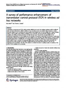
requires that there be communication schemes that enable the dynamic reuse of spectrum to support multiple users as they need it. Ad hoc networking is a proposed paradigm to solve this problem. In this paper, we present a new Medium Access Control (MAC) protocol, Synchronous Collision Resolution (SCR). SCR is unique as a contention-based access protocol since it does not resolve contentions based on the time of contention as is the case in Aloha and Carrier Sense Multiple Access (CSMA). In these protocols, a contending node gains access by being the only node amongst its neighbors to contend for access. These protocols make no effort to orchestrate the spatial reuse of a channel. Since they depend on regulating contention attempts so that just one node contends at a time, they are very susceptible to congestion collapse when the number of nodes contending exceeds the number for which the protocol is tuned. By contrast, SCR requires all contending nodes to participate in a signaling protocol. Through its synchronous signaling mechanism, SCR resolves a subset of nodes from a set of contending nodes, which are spatially separated from each other and, thus, can exchange packets simultaneously using the same radio channel. This distributed process achieves a high spatial reuse of the wireless channel and does not suffer from congestion collapse. This paper presents the seminal work of using synchronized signaling to resolve contentions in ad hoc networks. It is based on the original research first described in [1]. The benefits of synchronizing access attempts is well known (e.g. Slotted Aloha versus Aloha) and the use of signaling to resolve contention is also an established concept (e.g. HIPERLAN 1 [2]). The concept of synchronizing a signaling protocol across an ad hoc network to manage spatial reuse is a unique concept. The benefits of SCR are far reaching and several sequel stories have been published without this foundation. Included is its ability to manage low energy states for energy conservation [3] and its ability to provide quality of service [4]. Additionally, derivative work that modifies the originally suggested signaling scheme was presented in [5]. The work in this paper is unique in that it is the first attempt to quantify the ability of this mechanism to orchestrate the reuse of a wireless channel. Our methodology for characterizing the capacity of a MAC protocol across load and node density conditions is also unique. We start this paper with a very brief introduction to the protocol in Section 2. A common objection to synchronous protocols is that synchronization is too difficult to achieve. We discuss synchronization issues and show that adequate time synchronization can be achieved in Section 3. In Section 4, we provide a detailed discussion of the performance of SCR, discussing the ability of signaling to resolve contentions, to separate contending nodes in an ad hoc environment, to distribute the nodes for high capacity, and then to enable these nodes to exchange packets successfully. In Section 5, we identify an adverse condition that may befuddle the protocol and then propose an easy signaling technique that will resolve it. We discuss this technique’s effect on spatial capacity. Section 6 discusses SCR’s potential for further enhancement. Section 7 provides our conclusions. RTS CTS CR Signaling

Protocol Data Unit

ACK

Transmission Slot

… Fig. 1. The Synchronous Collision Resolution MAC protocol

2. Protocol Overview Figure 1 illustrates the SCR protocol. The radio channel is divided up into sequential transmission slots and then each transmission slot is broken up into a series of signals followed by the transmission of a protocol data unit (PDU). At the beginning of the transmission slot, all nodes

a.

b.

... c.

d.

Fig. 2. An example of Collision Resolution Signaling. All nodes start off as contenders in Panel a. Then, through a series of signals, two sets of which are illustrated in Panels b and c, a final subset of contenders is selected in Panel d. The large dots are nodes that view themselves as contenders, the small dots are nodes that view themselves as having lost the contention, and the large circles represent the range of the signals. Contenders defer when they hear the signal of another contender.

with packets to send contend for access to the medium by participating in a collision resolution signaling (CRS) protocol. The CRS protocol can follow many different approaches – Sections 4 and 5 will cover these in more detail. Here, we use a series of panels in Figure 2 to illustrate the desired outcome of CRS. In Panel 2a, we illustrate a situation where all nodes in the network start off as contenders, and then, through a series of signals, two sets of which are illustrated in Panels 2b and 2c, reduce these contenders to the final subset of the contending nodes illustrated in Panel 2d. The large dots are nodes that view themselves as contenders, the small dots are nodes that view themselves as having lost the contention, and the large circles represent the range of the signals. In this example, nodes randomly select signaling slots in which to signal at the beginning of the transmission slot and then defer from contending if they hear any other node’s signal. The surviving contenders are separated by at least the range of their signals. At the conclusion of the CRS, the surviving contenders attempt to execute a handshake with their destinations. These surviving contenders send a request-to-send (RTS) packet and if the destinations hear these RTS packets, they respond with a clear-to-send (CTS) packet. We emphasize that the role of this handshake is different than that of the RTS-CTS exchange used in the IEEE 802.11 MAC [6]. Rather than preempting other contenders, the RTS and CTS packets are sent simultaneously to verify whether the contenders can exchange packets with their destinations simultaneously. The panels of Figure 3 illustrate the process. In Panel 3a, the large nodes are the signaling survivors. The lines are drawn from the signaling survivors to the destinations to which they want to send packets. Circles are drawn around nodes that are broadcasting a packet. Panel 3b reveals those nodes that transmit RTS packets. The large circles are the ranges of their RTS transmissions. If a destination receives a RTS packet, it responds with a CTS packet, see Panel 3c. These CTS packets are also sent simultaneously. Note that the recipients of RTS packets for broadcasts do not respond. The source would not be able to distinguish CTS packets from multiple destinations. Next, if contenders receive a CTS packet, they become contention winners and transmit their

a.

b.

c.

d.

Fig. 3. Example of the RTS-CTS handshake finalizing the set of nodes to exchange packets: Panel a illustrates the set of contenders that survived signaling and their intended destinations (circles indicate intended broadcasts). Panel b illustrates the contenders’ simultaneous RTS transmissions. Panel c illustrates the destinations’ simultaneous response of CTS packets. Panel d illustrates the winners of the contention.

PDU’s. Finally, destinations respond to successfully received PDUs with an acknowledgement (ACK). We note that from the perspective of both the contention winners and their destinations, interference conditions can only get better through the deferrals that result from the RTS-CTS exchanges since PDUs and ACKs are transmitted with equal or lower power than that used for the RTS-CTS exchanges.3 As a result, contention winners should also be successful in exchanging their PDUs. The result of this protocol is a high density of nodes that can exchange PDUs simultaneously. A goal of this paper is to quantify the effectiveness of our protocol to achieve high “spatial” throughput. 3. Network Synchronization SCR requires that nodes be synchronized, indeed synchronized contentions and transmissions are key to its operation. The follow-on question, then, is how well must the network be synchronized for the protocol to work? The answer is “any reasonable level of synchronization.” We emphasize that the purpose of synchronization is to prevent ambiguity in identifying in which signaling slots signals are sent. However, there is a direct tradeoff between the degree of synchronization and the efficiency of the protocol since mis-synchronization must be accommodated with longer signaling slots and guard bands between transmissions. Appendix A illustrates how signaling slots can be sized to prevent ambiguity. Variance in synchronization is but one factor in sizing a slot; propagation delays, transceiver transition times between receive and transmit states, and the time a receiver must detect a signal to be certain one is present are additional factors that need to be considered. Thus, the protocol must be optimized for the specific physical layer with which it is used. Reciprocally, a physical layer can be designed to optimize the performance of SCR. 3

The RTS-CTS handshake can be used as a feedback mechanism for power control. Power may only be decreased.

The issue then, is, not what synchronization is required, but rather, what synchronization can be achieved. Synchronization can be provided by an external source or be generated internally. The obvious external source is the Global Positioning System (GPS). GPS provides a worldwide synchronization to a resolution of approximately 250 ns [7]. Considering that the time for a signal to propagate 300 meters is four times that value, synchronization would have only a small impact on the slot size. Other possible external sources for synchronization include position location awareness systems like the U.S. Army’s Enhanced Position Location Reporting System (EPLRS) or ultra wideband (UWB) radios. Both have timing resolution of at least 1 µs. In the case of UWB, manufacturers claim a resolution in the range of tens of picoseconds [8]. If the network operates in an environment where any one of these sources can be considered reliable, synchronization becomes the lesser issue in the sizing of signaling slots as compared to propagation times and transceiver transition times. Building a system that relies on an external source for synchronization may not be the most desirable design alternative. In a military communications application, a synchronization system such as GPS may be the most vulnerable part of the communications system. Not only can the GPS signal be jammed, but there are some environments in which it does not operate. Thus, it would be preferable if synchronization could be achieved by the communications system itself. We claim that SCR’s synchronous character gives it this very capability. The popular notion that synchronization is difficult to achieve in an ad hoc network is based on the experience of using wired network protocols like the Network Timing Protocol (NTP) to achieve this synchronization. This type of protocol achieves synchronization by timing the round trip times of packets between source destination pairs. The level of synchronization that can be achieved is limited by various sources of non-determinism. The sources of non-determinism can be identified by tracking the sequence of events. A packet is formed, the node accesses the channel through the MAC, the signal propagates to the destination, the destination processes the packet, and then the destination repeats the steps in making a reply. Each of these steps can contribute to variability, especially asynchronous MAC protocols that use time to resolve contentions. Additional non-determinism comes from the drift and instability of clocks at nodes. The broadcast medium together with the use of a synchronous access protocol can resolve or reduce all of the sources of non-determinism. Elson et. al. [9] demonstrate that broadcasted messages alone can reduce the effects of clock drift and instability and achieve synchronization of a few microseconds despite the underlying access protocol. Synchronization is achieved by sharing information amongst nodes that receive the same broadcast. These methods, however, do not eliminate the non-deterministic factors associated with propagation which are a more dominant factor as transmission ranges increase. The methods to remove the uncertainty of propagation delays are the same as those used to develop location awareness. Broadcasts from known locations that occur at known times are used by other nodes to resolve their locations and their clocks. These multilateration algorithms are the foundation of the GPS, EPLRS, and UWB synchronization methods. For example, in EPLRS, two nodes are surveyed into position (i.e. placed in locations known to each other) with one node serving as the master clock. Since locations are known, propagation times are known. The two nodes become synchronized through the exchange of packets. Then, other nodes use these two nodes and each other to resolve their location and timing. The U.S. Army’s operational testing of this system determined that its effectiveness improved as the number of nodes in the system increased. Systems employing SCR could, if necessary, easily incorporate location awareness algorithms. Packets are sent at known times so timestamps attached to packets can be set to match the time of transmission. Location information can be included in packet overhead. Thus, every packet, (i.e. RTS, CTS, PDU, and ACK) can serve as a synchronization and location awareness message. As a system, we would expect the plurality of nodes to achieve high synchronization and location awareness just as in EPLRS. Upon initialization, a network could synchronize to any of the following: GPS, a small number of nodes equipped with GPS, or a small number of nodes in surveyed positions. Of great importance to military networks is the availability of a reliable backup system to retain synchronization and location awareness in a hostile environment where

GPS could be attacked. The combined use of external synchronization sources and internal algorithms that is possible with SCR enables the rapidly deployable and robust system that is desired. 4. Protocol Performance Access protocol performance in ad hoc environments has several dimensions. These dimensions include how well the protocol resolves contention, how well it enables the reuse of the channel, how well it operates in a congested environment, and whether the protocol provides fair access. In this section, we provide an analysis of the performance of SCR with respect to each of these criteria. 4.1 Local Collision Resolution Local collision resolution performance is measured as the probability that one node from amongst multiple contending nodes will win a contention when all contenders are within range of each other. We provide an overview of CRS options and a model to predict their performance and to use in their design. CRS methods consist of consecutive signaling phases and signals which we call assertion signals. The signaling phases may have one or multiple signaling slots. We assume that a receiver can detect the presence of assertion signals, irrespective of the number of nodes that are simultaneously transmitting them. A node survives CRS by surviving all signaling phases. A node survives a signaling phase by not being preempted by another node’s assertion signal according to the preemption rules of the signaling phase. Signaling phases may be one of two types, first-to-assert and last-to-assert. As the names imply, in first-to-assert phases the node that sends a signal first survives and in the last-to-assert phases the node that sends a signal last survives. A contending node that hears another node contend prior to itself in a first-to-assert phase will stop contending. A contending node that hears another node contend after it has already signaled in a last-to-assert phase will stop contending. Assertion signals may be one of two types, discrete or continuous. Discrete signals are sent within the space of a single signaling slot. Continuous signals may occur across several slots. In first-to-assert phases, an assertion signal would begin at the selected slot to start signaling and continue until the end of the phase. In last-to-assert phases, the signal would begin at the beginning of the phase and end at the selected slot. Figure 4 illustrates the difference between these signaling methods. In this example, the first and third phases are first-to-assert and the second phase is last-to-assert. ... Phase 1

Phase 2

Phase 3

...

a. Continuous signaling

... Phase 1

Phase 2

Phase 3

...

b. Discrete signaling

Figure 4. Comparison of continuous and discrete signaling

One designs a signaling phase by choosing the number of signaling slots and the signal selection probabilities, i.e. the probability that a contender will assert himself in a given slot. A contending node chooses to transmit an assertion signal on a slot-by-slot basis during a phase. A contender will only send one assertion signal and may choose to send none, so for m slots there are

m+1 possible signals.4 We denote the probability that a node will select signal i by pi . The last assertion signal of the series has probability 1. The option to not signal is equivalent to the last signal in a first-to-assert phase or the first signal in a last-to-assert phase. For a given phase design we denote the set of assertion signal probabilities by p x = ( p1x , p2x ,?, phx−1 ,1) , where h-1 is the number of slots in signaling phase x. Let Hx be a random variable denoting the assertion signal which a typical contender asserts himself during signaling phase x, then for a vector of assertion probabilities px we have i −1

Pr ( H x = i ) = pix ⋅ ∏ (1 − p xj )

for i=1,2,? h .

j=1

Suppose that Kx nodes within range of each other are contending during signaling phase x, and let

S xf and Slx be random variables denoting the number of survivors for this phase if it operates on the first-to-assert or last-to-assert principle. probabilities of survivors as follows

In this case we can determine the conditional

(

)

0 d ijn + d njk + c

(5)

where n is the exponent of the log distance path loss model, [17], d ik is the distance between nodes i and k, and c is a constant representing the power used by the intermediate node to receive and process a packet. Figure 12a illustrates that a boundary can be drawn for every S-D pair where the destination is an energy efficient relay for all nodes beyond the boundary. Such boundaries can be drawn for all destinations. As illustrated in Figure 12b, the relay boundaries of a source’s closest neighbors will enclose the source. This next hop strategy only uses neighbors within this boundary and we call it enclosure hopping. 1.2 1.0 0.8

Normal

UA

NFP

0.6

Enc losure

0.4 0.2 0.0

1

1.1

1.2

1.3

α

1.4

1.5

1.6

1.7

Figure 13. Comparison of exchange densities of different routing strategies using the CRS design of Figure 10a

We conducted simulations of three routing strategies: the “normal” configuration simulated for Figure 11, NFP, and enclosure-hopping. In the NFP simulation, a direction was selected at random and then the node meeting the NFP criteria was selected as the destination. In enclosure hopping, a node within a transmission area is selected at random and then the node within the enclosure that is closest to the destination is selected as the next hop. The enclosure nodes were determined using the criterion of (5) with a path loss exponent of 4 and a reception constant equivalent to the energy required to transmit a packet a tenth of the transmission radius. Although energy conservation implies reduced transmit power, we used the maximum transmit power for all transmissions. Figure 13 illustrates the simulation results of the two routing strategies described in this section as compared to the normal strategy. We see that both next hop strategies dramatically improve the spatial usage of SCR.

Enclosure

Normal 0.3

Normal

0.4

Enclosure

dFP

dFPA0.2 NFP

0.2

NFP 0.1

0

0

5

10

15

20

σA

0

30

25

a. Forward progress per transmission

0

5

10

15

20

ρ σ A

25

30

b. Forward progress per slot per transmission area

Figure 14. Packet progress as a function of node density in a transmission area using the CRS design of Fig. 10a, α = 1.3 (Transmission radius remains constant and density increases. )

0.8

0.6

0.6

Normal dFPA

dFP 0.4

Enclosure

0.4

Normal

Enclosure

NFP

0.2

NFP

0.2

0

0.5

0

r 5

1.5

1

8 10

15

20

σA a. Forward progress per transmission 2

25

0

0.5

0

r 5

1.5

1

8 10

15

20

25

σA b. Forward progress per slot per π square units area 2

Figure 15. Packet progress as a function of adjusting transmission radii using the CRS design of Fig. 10a, α = 1.3 (Density remains constant but σ A changes since the transmission radius changes. In these graphs σA = 10 at r = 1. Decreasing transmission range increases spatial usage faster than it decreases the forward progress per transmission so total forward progress per slot increases.)

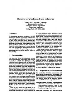
Spatial usage is not the best measure of capacity since by choosing to traverse shorter hops, packets do not progress as far in the network. Therefore, we evaluated the effectiveness of these techniques considering forward progress. Forward progress for the random routing method is the distance of the exchange, for the NFP technique it is the forward progress in the direction of the destination illustrated in Figure 11, and for the enclosure hopping technique it is the distance in the direction of the randomly selected destination. We denote forward progress per transmission as dFP. Our measure of effectiveness is forward progress per transmission area and we denote it as dFPA. Figure 14 compares the routing strategies under these measures. NFP is clearly the least effective strategy. Although enclosure hopping greatly increases the density of exchanges, there is only a small increase in dFPA because of the reduced forward progress. The results in Figure 14 also indicate that node density does not decrease the capacity. In practice, however, it may be desirable to select the network density by adjusting the transmit power used by the nodes. In Figure 15, we present the data of Figure 14 where we consider node density fixed and then vary the transmission radius to determine the degree of the network. As seen, lower densities yield greater average forward progress. Therefore, we conclude that the optimum node density is the smallest density that keeps the network connected.

σA = 25 1.5

1.5

σA = 25 σA = 20

1

UA

σA = 5

σA = 15 σA = 10

0

1

0

0.5

σA = 10 σA = 5

UA

σA = 2

0.5

σA = 20 σA = 15

1

λA a. Normal hopping

1.5

σA = 2

0.5

2

0

0

0.5

1

λA

1.5

2

b. Enclosure hopping

Figure 16. Spatial capacity as a function of load and node density using the CRS design of Figure 10a

Up to this point in our discussion, we have considered all nodes to be contenders all the time. In our final analysis of the spatial capacity, we consider the effect of load where all nodes may not be contending simultaneously. We define load as the rate packets arrive to a transmission area and denote it as, λA. One packet arrives to a transmission area per transmission slot when the arrival rate is λA = 1. In our simulation, we evenly distribute these arrivals to the nodes in the network. Figure 16 illustrates the density of exchanges as a function of load and node density for the normal and enclosure routing strategies. The results demonstrate that the protocol remains stable up to the maximum spatial capacity. It further demonstrates that excess load will not decrease capacity. 4.6 Observations We have provided a comprehensive evaluation of the issues that are associated with spatial capacity. We have demonstrated that SCR is very robust and can be designed to remain so for any density of contenders. We have demonstrated that signaling distributes contenders and that through this distribution other techniques can be used to increase capacity. We also demonstrated that routing strategies improve capacity. We have demonstrated that the protocol is stable and does not suffer congestion collapse. Although not explicitly described there are additional observations: CRS signaling has no memory and unlike the backoff strategies of CSMA type protocols, which do, will never give preference to any node in signaling unless signaling is designed to do so. Thus, SCR is fair. Since access attempts are simultaneous, the perpetual deferrals that may occur with exposed nodes will never occur.6 Since CRS is a separate process from the exchange of packets, power level can be used to select the separation distance between contenders, thus creating more optimum conditions for packet exchanges. Any technique that improves capture will improve capacity making this protocol complementary to physical layers that use directional antennas or different channels for data exchange. We conclude with the fact that we have used five measures to quantify spatial reuse: separation distance of surviving contenders, density of surviving contenders, distribution of surviving contenders, density of packet exchanges, and density of forward progress of packet exchanges. Key to all of these measures is that they relate to the local perspective of a single node and its transmission area and the parameters that affect that node locally, i.e. density of neighbors and load at those neighbors. We show that SCR creates conditions such that the protocol’s performance remains the same regardless of how far the network extends beyond the node’s range. 6 Exposed nodes occur when carrier sensing protocols are used. An exposed node is a node that hears two disjoint partitions of a network and must wait for both partitions to be silent before contending for access. In highly loaded networks, such nodes may never have the opportunity to gain access.

This perspective is different and we believe more appropriate than that presented in [18], where network-wide capacity is considered. The premise of this latter analysis is that any node is equally likely to communicate to any other node in the network. Inevitably, in a network-wide analysis of this type, the conclusion is that capacity will decrease with an increase in the number of nodes. We believe ad hoc networks will tend to be heterogeneous consisting of other long range networking components that will be used to selectively remove traffic that would load many regions of the underlying wireless network. Under such conditions, an understanding of local performance is the more useful as it identifies when load will exceed the underlying regional capacity of the wireless network thus requiring the use of these other network components. 5. Responding to Adverse Conditions CRS, as described, may resolve to a subset of contenders that may block each other at a common destination. Blocking occurs when two contenders gain access to the channel and attempt to send a packet to the same destination. If these nodes continuously gain access the result can be deadlock unless some mechanism is in place to break it. Note that the condition for deadlock to occur is that the same nodes must continuously gain access. This implies there are no contenders within range for them to interact with (including each other), or else it would be unlikely that they would repeatedly gain access together. Thus, deadlock is most likely to occur in low-load and low-density networks. Deadlock can be broken by a signaling technique called echoing. In echoing, nodes that hear signals echo them in the next signaling slot of the same signaling phase. Echoes clear a range up to two hops from the contender that sends the assertion signal. In this manner, surviving contenders clear other contenders one hop beyond all potential destinations. Figure 17 illustrates the effect of echoing. Echoing may be a permanent part of the signaling design or optionally executed to break deadlock when it is detected. The mechanism that would trigger this change in signaling is beyond the scope of this paper. Our goal is to determine the effect of echoing on survivor density and so we evaluate the performance of a CRS design that uses echoing all the time.

a.

b.

Figure 17. Illustration of echoing. In panel a, two nodes send assertion signals and then in panel b those nodes that hear the assertion signal echo it. All contenders within range of the assertion signal and the echoes that did not transmit an assertion signal defer from contending.

The advantage of echoing all the time is that survivors have a high probability of sending packets to destinations without blocking or interference7 and thus RTS-CTS handshakes can be dropped. The disadvantages of echoing all the time are that it uses more signaling slots per phase and that it may result in a sparser subset of survivors. We explored its effect on survivor density and contender separation in the same simulation environment as we used previously. Our CRS design with echoing was based on that presented in [5]. This design uses 2-slot signaling phases 7

Interference may still occur unless destination echoes are heard by all contenders within the interference range.

where the second slot in each phase is just for echoing. That is, in each phase, a contender makes the choice to signal or not to signal. As before, if a contender signals, it survives the phase. If a node does not signal but hears an assertion signal, it defers from contending and then echoes the signal it heard in the very next signaling slot. If a node does not signal, does not hear an assertion signal, but hears an echo, it will also defer from contending. As this technique can be quite aggressive at thinning out the contenders, [5] recommends an intermediate promotion phase to reactivate some contenders. In this promotion phase, all contenders that are still survivors signal and, as before, all nodes that hear the signal echo it. Contenders that have deferred due to hearing an earlier signal but do not hear either the assertion or echo signals of the promotion phase reactivate and continue to contend. This signaling design consists of two series of phases used to reduce the number of contenders separated by the promotion phase. We use two 12 phase series with px = 0.5 for all phases which was shown to produce good performance in [5]. 0.8 0.12

Fraction of Survivors

0.6 0.5 0.4 0.3 0.2 0.1 0

10

0.08

2 5 8 10 15 20 25

25

20 0.1

15

8 5

0.06

2 0.04 0.02

Contender Density,

a. Simulated survivor densities

4.00

3.50

25

3.00

σA

20

2.50

15

2.00

10

1.50

8

1.00

5

0.50

0

2

0.00

Survivor Density, S A

0.7

Fraction of Range

b. Density of range to the nearest surviving neighbor

Figure 18. Performance of CRS using echoing when all nodes are contenders. Only survivors with neighbors are considered in the graphs, so the 32% of survivors that had no neighbors when σA = 2 are not included in the results shown in a or b. This explains the low survivor density for σ A = 2 in a.

Figure 18 illustrates the performance of this CRS design with echoing. Figure 18a shows that the density of surviving contenders decreases with increasing node density. (Note that CRS designs that use echoing will have performance based on node density rather than contender density since all nodes participate in signaling.) Figure 18b shows that the separation distance between the surviving contenders increases with node density. These results are expected. The cause of the decreased capacity and increased average separation distance is that with a greater density of nodes, echoing will originate from more sources in the transmission area of the asserting contender and thus echoing will be heard over a larger spatial region of the network. In the limit, echoing should suppress all contenders up to a distance of two transmission radii from the surviving contender. Figure 18b begins to illustrate this limit as the curves are becoming more tightly centered around a range of 2.00 as node density increases. The lower density and tighter compaction of surviving contenders for low node densities occurs because it is more likely that neighboring contenders will not have a third node between them that can relay echoes. While this decrease in separation may appear on one hand to result in a greater likelihood of interference, echoing is still providing a benefit by preventing blocking and collisions. In fact, at lower densities, it is more likely that hidden nodes will choose the same destination and so echoing is more necessary to prevent the resulting blocking problem. Although the density of surviving contenders when echoing is used is less than that of signaling without echoing it possesses some definite advantages. Most of the contention survivors will be able to successfully exchange packets since echoing clears away most potential interfering nodes. Thus, routing strategies would have less effect on spatial usage and average forward progress per transmission will be greater. Echoing would be better suited for use with routing

protocols that use hop count as the cost of a route. On the other hand, echoing offers less opportunity for increasing capacity using physical layer techniques that improve capture. 6. Enhancements The synchronous nature of SCR, the ability of one node to preempt others through signaling, and the geometry of surviving contenders after signaling all contribute to many exciting possibilities that we have already started to explore. We have already argued that the synchronous access mechanism provides a foundation upon which network synchronization and location awareness can be made integral to the access protocol. Our research has also identified ways this mechanism can be used to conserve energy [1, 3], provide priority access such that contenders with the highest priority packets get precedence in gaining access [1, 4], provide resource reservation for real time streams [1, 4], and coordinate the use of multiple channels in a flat network [1, 4]. We are currently considering the use of echoing to coordinate the use of sectored antennas. The final distribution of surviving contenders that results from CRS can be best described as a random cellular network where survivors, like base stations, are separated from each other and numerous non-contending nodes, like cellular phones, are within their range. This geometry enables the exploitation of technologies that have been developed for cellular telephony. Code division multiple access (CDMA) and smart antennas may be used to further increase the capacity of ad hoc networks. 7. Conclusion This paper has two main contributions, it introduces a medium access control protocol for ad hoc networks that has high capacity and it provides a methodology to evaluate capacity and spatial reuse. We introduce the contention based access protocol, Synchronous Collision Resolution, which arbitrates access to a shared wireless channel using synchronous signaling and have demonstrated that this technique provides a distributed mechanism that orchestrates spatial reuse of the channel and achieves high capacity. We believe that the techniques we have put forward in this paper are appropriate for many classes of wireless ad hoc networks. The issues associated with the time synchronization requirements of these techniques are straightforward, and may be managed in a number of different ways at the discretion of the designer. We suggest that these techniques are applicable to various networks of different degrees of sophistication, noting that single channel radio networks might benefit greatly from CRS designs that use echoing, while networks with more sophistication might be able to operate with higher survivor densities and use techniques such as CDMA and smart antennas to ensure non-interfering transmissions. We have developed multiple measures to evaluate a MAC protocol’s ability to orchestrate spatial reuse and to achieve high capacity. We provided a methodology to characterize the performance of a MAC protocol using these measures across a range of conditions including node density and traffic load and applied it to SCR. Although others have used a similar geometric approach to evaluate performance it has been used to optimize not characterize MAC protocols. [11-15] Additionally, their optimizations have allowed load and node density to be independent variables thus providing dubious conclusions since both these variables are virtually uncontrollable in an ad hoc environment and have a significant impact on capacity when varied in networks using Aloha and CSMA MAC protocols. On account of this lack of a performance characterization we were unable to compare SCR’s performance to that of other MAC protocols. We plan to do such a characterization of the 802.11 MAC protocol in our future work. Appendix A, Selecting Signaling Slot and Guard Band Sizes for Discrete Signals As a starting reference, we assume nodes will always start sending their signal at the start of a signaling slot and stop at the end. Signal slot sizes are chosen to prevent any ambiguity as to in which signaling slots signals occur. The objective in signal slot sizing is to select the values of the

design parameters listed in Table A2 such that portions of signals that arrive in the wrong slot τsn are not detected as signals while the portions that arrive in the correct slots, τss, are. Ideally, τss is always larger than τsm, the minimum time to detect a signal is present, and τsn is always less, however, this may not be the case and so signals and the minimum detection time, tsf or tsl, are made longer. τp

tS

τrt

τss

tS

τp

τsn

τsn τsy

tS

τsy

a. Effect of a delayed first-to-assert signal tS

τtr

τss

τrt

tS

b. Effect of an early first-to-assert signal

τsn

τp

tS

τsn

τsy

τsy

τp

c. Effect of a delayed last-to-assert signal

τtr

τss

d. Effect of an early last-to-assert signal

Figure A1. Timing in first to assert and last to assert signaling slots

Table A1. Timing constraints and results that affect signal slot size

τp τrt τtr τsy τsm τsn τss

Propagation delay between nodes displaced the maximum receiving distance from each other Maximum time required by a transceiver to transition from the receive to the transmit state Maximum time required by a transceiver to transition from the transmit to the receive state Maximum difference in the synchronization of two nodes Minimum time to sense a signal in order to detect its presence Time a node senses a signal in the wrong slot Time a node senses a signal in the correct slot Table A2. Design parameters

tS tsf: tsl tg

Duration of a slot Selected minimum time to sense a signal in a first to assert slot to detect it. Selected minimum time to sense a signal in a last to assert slot to detect it. Guard time between phases

In Figure A.1, we see that the critical point at which false detection occurs in first-to-assert signaling is when a signal is sent early and the signal must not be detected early by a node that intends to signal in the same slot. The critical correct detection occurs when the signal is sent late and must be detected by a node that intends on signaling in the next signaling slot. Thus, the design equations are

(

tsf > max τ sy − (τ rt + τ p ) ,τ sm

)

and t S > τ sy + τ rt + τ p + tsf .

Similarly, in last-to-assert signaling, we see that the critical point at which a false detection occurs is when a signal is sent late and another node has signaled in the same slot. The critical correct detection occurs when a signal is sent early and another node has sent a signal in the preceding slot. Thus, the design equations are tsl > max (τ sy + τ p − τ tr ,τ sm )

and t S > τ sy + τ tr + t sl − τ p .

Last to assert signaling slots can be made smaller than first to assert signaling slots. tS

tg

τsn

tS

τp

τsn

τsy

a. Effect of a late signal

τp

tg

τ sy

b. Effect of an early signal

Figure A2. Timing across signaling phases

In our selection of slot sizes and signal duration we were not concerned that a late first to assert signal may also be detected in a slot after the intended signaling slot or that an early last to assert signal is also detected in an earlier signaling slot than intended. However, these two conditions are important between phases. Figure 2A illustrates the timing effect. We see that the late signal governs the sizing of the guard time. The guard time should meet the following criterion. t g > τ sy + τ p − tsf . Appendix B, Comparison of the Protocol and Physical Capture Models Interference from neighboring sources may be modeled by either a protocol model or a physical model. Let Ys denote the location of a source node, Yd denote the location of a destination node, and (Yi , i∈Κ) denote the locations of the subset of nodes transmitting simultaneously on the same channel. In the protocol model, a transmission is considered successful when (B.1) Yi − Yd ≥ α ⋅ Ys − Yd , Ys − Yd < R for all Yi, (i ≠s), where α denotes the interference ratio and R is the maximum range to a destination to which a source will transmit. Using the physical model, a transmission is considered successful when

Ps n

≈ Ys − Yd ’ Δ ÷ Δ d ÷ r « ◊ Pi 1 No + PG i∈K ≈ Y − Y i d i≠ s Δ Δ d r «

≥β

ƒ

n

’ ÷ ÷ ◊

where No is the ambient noise, PG is the processing gain, Pi is the effective radiated power from node i measured at the reference distance dr, n is the path loss exponent, and β is the minimum signal to interference ratio (SIR). We assume that collision resolution signaling is effective at separating contenders such that no surviving nodes are closer than R to each other and the closest node is the dominant interfering node. Thus, the condition for transmission success can be approximated by Ps n

≈ Ys − Yd ’ ÷ Δ Δ ÷ « dr ◊ Pi No + ≈ Yi − Yd PG Δ Δ d r «

≥β

(B.2)

n

’ ÷ ÷ ◊

where Yi is the location of the closest interfering node. Let x units be the range to a destination and let γx units be the minimum range from an interfering node to this same destination that will still meet the SIR criterion β. By (B.2), we observe that if No and n are constants, γ x1 γ x2 < , ∀x1 < x2 . In other words, as x, the distance between the source and destination, x1 x2 decreases, No becomes less and less dominant resulting in an interferer to destination distance, γx , that decreases more and more rapidly. The result is that there is a corresponding decrease in the interference ratio as x decreases. Let us then define α =

γR R

where R is as defined before. This

selection of the interference ratio will be larger than the interference ratio for any x < R. By using this value of α in (B.1), we have established a conservative model for interference for ranges x < R. In real systems, n may become smaller normally breaking from n = 4 to n=2 when distances are within the Fresnel zone [19]. Since we assume the network will operate at ranges beyond the Fresnel zone it is also reasonable to assume that interfering nodes will never be within the Fresnel zone while retaining the interference ratio a and the minimum separation distance R. (e.g. When operating at 2.4 GHz with antennas 1.7 meters above the ground, the Fresnel zone is within 100 meters of a transmitting node.) Thus, the protocol model remains a conservative model for our analysis. Practical values for α depend on the physical layer. The interference ratio for average capture with frequency modulated communications is α = 1.3 [13]. The interference ratio of the 1Mbps signal specified in the 802.11 Direct Sequence Spread Spectrum physical layer specification can be calculated using (B.2). Each data bit is spread by an 11 chip pseudo-noise sequence that provides an approximate processing gain of PG = 11.8 Assuming a maximum transmission range

8

A PG = 11 occurs if the chip sequence of the interfering signal is not aligned with that of the source’s signal.

of 300 meters, an effective radiated power of 3.9 x 10-8 Watts at 100 meters9, ambient noise of -95 dBm,10 and a minimum SIR of 10 dB, the corresponding interference ratio is α ≈ 1.0. Appendix C, Calculating the Interference Free Zone Area In this appendix we derive the calculation for the area of the interference free (IF) zone of a transmitting node in a triangular tessellation, C(x,α). We define the clear zone as the region that a destination can receive a transmission from a source node without interference from an adjacent node that is also transmitting. We assume a protocol capture model as defined in Appendix B. If a destination node is further than α times the distance to the source node from all other transmitting

1 φ1

x

α φ2

αy

y π/6

φ2 x

Capture Interface

a. φ1