Feb 19, 2015 - sum of RBNS (reported but not settled) and IBNR (incurred but not reported) claims by accident years and development years under the ...
International Journal of Contemporary Mathematical Sciences Vol. 10, 2015, no. 2, 65 - 77 HIKARI Ltd, www.m-hikari.com http://dx.doi.org/10.12988/ijcms.2015.515
A Simple Multi-State Gamma Claims Reserving Model Werner Hürlimann Feldstrasse 145, CH-8004 Zürich, Switzerland Copyright © 2015 Werner Hürlimann. This is an open access article distributed under the Creative Commons Attribution License, which permits unrestricted use, distribution, and reproduction in any medium, provided the original work is properly cited.
Abstract We construct a simple parametric multi-state gamma distributed aggregate claims reserving model. It is based on the multi-state claims number reserving model by Orr [9], and adds the simplest possible modelling of the claims size process. Predictive power and advantages of the new model are discussed and illustrated. Mathematics Subject Classification: 62P05, 60J28, 91B70 Keywords: claims reserve, IBNR reserve, RBNS reserve, gamma distribution
1. Introduction The present contribution is a synthesis of previous work by Orr [9] and the author [6]. It is devoted to the construction of a simple parametric multi-state gamma distributed aggregate claims reserving model, which is sufficiently flexible to allow for a full stochastic simulation of the aggregate claims reserving process. It retains the simple features of the multi-state claims number reserving model of Orr [9] and adds the simplest possible reasonable modelling of the claims size process. It is important to emphasize the advantages of the new model over the previous gamma model from the author. The latter allows for a stochastic prediction of the future aggregate claims reserves, however only at the level of the sum of RBNS (reported but not settled) and IBNR (incurred but not reported) claims by accident years and development years under the assumption that after the fixed observable number of development years all claims that occurred during an accident year are known and closed. In contrast, the new multi-state reserving
Werner Hürlimann
66
model allows for a stochastic prediction of all the main claims reserving components including claim numbers and separation into RBNS, IBNR and PAID claims at the additional level of both claim numbers and claim sizes. Furthermore, the new model is not restricted by an assumption on the number of development years. A brief account of the content follows. Section 2 recalls how the multi-state claims number reserving model by Orr [9] is obtained from a multi-state Markov chain modelling of the claims reserving process along the line of papers including Hachemeister [3], Norberg [8] and Hesselager [4]. Section 3 presents the simplest extension to a multi-state aggregate claims reserving model with gamma distributed claim sizes, which can be approximated for sufficiently large portfolios by a gamma distributed aggregate claims reserving model. Section 4 links the model of Section 3 with the previous model in [6]. Since both models assume gamma distributed paid claims, an obvious comparison is done by equating the mean and variance of the paid claims over the given number of observable development years. By this way the parameters of the new gamma model are simple functions of the parameters of the previous model, which can be estimated using the method of maximum likelihood. Moreover, the new gamma model is independent of the Poisson arrival rates of the claims number process, and as a consequence it turns out that the approximation made for sufficiently large portfolios coincides in distribution with the original multi-state gamma model. Finally, in the last Section 5, we compare the new multi-state gamma claims reserving model with the previous gamma model using the published loss triangle of paid claims and exposures in Mack [7]. The stochastic prediction power of the new model is illustrated and discussed.
2. Orr’s multi-state claims number reserving model revisited The modeling of claims development using a multi-state approach has been discussed by Hachemeister [3], Norberg [8] and Hesselager [4]. Restricting the analysis to claim numbers, Orr [9] presented a quite simple stochastic claim number reserving model, which is our starting point. Consider the 3-state model 12 (v )
01 (u)
0 ~ IBNR
1 ~ RBNS
2 ~ PAID
"Unreported"
"Unsettled"
"Settled"
with state space S 0,1,2. Losses from an insurance portfolio are assumed to arrive in state 0 as Incurred But Not Reported (IBNR) claims or “Unreported” losses. These losses are then reported in state 1 as Reported But Not Settled (RBNS) or “Unsettled” claims, which are subsequently “Settled” in state 2 as paid (PAID) claims. The sum of RBNS and PAID claims is called “reported claims” while the sum of IBNR and RBNS claims is called “claims reserve”. We assume
A simple multi-state gamma claims reserving model
67
that the claims arrive as a Poisson process with a constant arrival rate during a given accident year. The development of a claim from occurrence until final settlement is assumed to be the realization of a time-inhomogeneous, continuoustime Markov chain. Let U be the “unreported waiting time” until notification with distribution function FU u PU u and let V be the “unsettled waiting time” from notification until final settlement with distribution function FV v PV v . By the Markov assumption, the transition rates from IBNR to RBNS and from RBNS to PAID are given by (e.g. Bowers et al. [2], p. 49):
01(u )
fU (u ) , FU (u )
f (v ) 12 (v) V , FV (v)
fU (u )
d FU (u ), FU (u ) 1 FU (u ), du
d fV (v ) FV (v), FV (v) 1 FV (v). dv
(2.1)
One is interested in the number of claims in state s from a given accident year at time t , which is denoted here by N s, t . In practice, only claims in states 1 and 2 can be observed, and this only up to the current time of observation. The actuarial challenge consists to estimate the number of unreported (hence unobserved) losses in state 0, corresponding to the IBNR claims. We derive general integral expressions for the expected numbers of claims in each state at an arbitrary time t and then specialize to Orr’s model. For this, one has to distinguish between the accident year itself and subsequent “run off” years. During the accident year (that is t 1 ), losses can arrive in state 0 and transition as claims to states 1 and 2. After the end of the accident year (that is t 1 ), no further losses can arrive, as they will attach to future accident years, but transitions will continue until all the claims have reached state 2. Case 1: t 1 Sub-case 1a: losses in state 0 at time t The expected number of losses in this situation is determined by the constant Poisson arrival rate at time s and the probability of staying in state 0 up to time t under the distribution function FU u through integration over all values of s between 0 and t : EN 0, t FU t s ds . t
(2.2)
0
Assuming an exponential unreported waiting time with average waiting time a, one gets
EN 0, t Sub-case 1b: claims in state 1 at time t
a
1 e . at
(2.3)
Werner Hürlimann
68
The expected number of claims in state 1 by time t , with losses arriving at time s and being reported at time r is obtained through integration as follows: t t
E N 1, t 01( r s )FU r s FV t r drds .
(2.4)
0 s
Assuming besides the preceding exponential unreported waiting time an exponential unsettled waiting time with average waiting time b, one gets
E N 1, t
1 e . 1 e a bb a b bt
at
(2.5)
Sub-case 1c: claims in state 2 at time t The expected number of claims in state 2 by time t is obtained through integration by considering losses at time s , which are reported at time r and settled at time q : EN 2, t 01(r s)FU r s 12 (q r )FV q r dqdrds . t t
t
0s
r
(2.6)
In the special case of exponential unreported and unsettled waiting times one gets
t 1 e at 1 e bt 1 e at EN 2, t a . a bb aa b a2 a
(2.7)
The formulas (2.5) and (2.7) hold for b a , which in practice can always be assumed through numerical approximation. Case 2: t 1 For t 1 , no further losses for the given accident year can occur and the “run-off” claims follow a pure multi-state Markov chain. Applying Kolmogorov’s forward equations, the expected numbers of claims in each state at time t 1 are determined by the formulas EN 0, t EN 0,1 p00 t 1,
EN 1, t EN 0,1 p01t 1 EN 1,1 p11t 1,
(2.8)
EN 2, t EN 0,1 p02 t 1 EN 1,1 p12 t 1 EN 2,1, where pij t 1 is the probability of being in state i at time 1 and state j at time t 1 . In the special exponential case the transition probabilities are given by
A simple multi-state gamma claims reserving model
p00 t 1 e a t 1 ,
p01t 1
p02 t 1 1 e a t 1 p11t 1 e b t 1 ,
69
a e b t 1 e a t 1 , a b
a e b t 1 e a t 1 , a b p12 t 1 1 e b t 1.
(2.9)
3. Extension to multi-state gamma aggregate claims reserving As pointed in [9], Section 7.4, the multi-state claims number reserving model can be readily extended to an amounts basis. Though the reporting and processing times of claims may depend strongly on the involved claim sizes, our multi-state aggregate claims reserving model is based on the following simplifying assumptions (A1)
(A2)
(A3)
For each accident year i 1,..., n assume a 3-state claims number model with Poisson arrival rate i and exponential unreported and unsettled waiting times with average waiting times a i and bi as in Orr’s model For each accident year, the state and time dependent claims numbers are independent from the claim sizes and the claims numbers of different accident years are also independent For each accident year i 1,..., n the (final) claim sizes are independent and identically distributed and known when claims are reported (no distinction between RBNS and PAID claim sizes) and they are gamma distributed with parameters ci , d i
A simple model like this only captures some main features and its limitations must always be emphasized in practical applications. On the other hand, the main advantages of a simple model are parsimony in the number of parameters, easier interpretations of the results and analytical tractability for statistical parameter estimation, numerical evaluation and Monte Carlo simulation. Let the random variables Ni s, t represent the number of claims arising from the accident year i 1,..., n in state s at time t . From the assumptions (A1) and (A2) one knows that the N i s, t , i 1,..., n, s 0,1,2, are independent i s, t EN i s, t Poisson distributed random variables with parameters determined by formulas of the type (2.3), (2.5), (2.7)-(2.9). Let the random variable Yi represent the independent and identically distributed claim sizes arising from the accident year i 1,..., n given a claim is in state 1 or 2. Furthermore, let the random variables X i s, t represent the aggregate claims arising from the accident year i 1,..., n in state s at time t . Then the random variables
Werner Hürlimann
70 Ni s ,t
X i s, t Yij , i 1,..., n, s 0,1,2, Yij ~ Yi j 1
(3.1)
are independent compound Poisson gamma distributed with mean and variance
i s, t EX i s, t i s, t ci / d i ,
i2 s, t Var X i s, t i s, t ci 1 ci / d i2 .
(3.2)
Let us assume that for sufficiently large values of i s, t the distributions of the random variables (3.1) can be approximated by gamma distributed random variables with parameters i s, t , i s, t determined by
i s, t i s, t ci /(1 ci ), i s, t di /(1 ci ).
(3.3)
This approximation is well-known and asymptotically exact as i s, t (e.g. [5]). In fact, through further specification, we construct in Section 4 a model such that (3.3) is independent of the Poisson arrival rates i by showing that (3.3) depends in the considered model only on the ratios i s, t / i , that is the gamma
approximation (3.3) of (3.1) is identical to its asymptotic limit as i s, t , hence the distributions defined by (3.3) and (3.1) coincide. This is an additional attractive feature of the proposed model.
4. A simple multi-state gamma claims reserving model The first part of the following development, which is independent from the preceding analysis, is inspired from the ideas presented in [6]. The total ultimate claims of the claims incurred in a given accident year, known in the future when all claims have been closed and paid out, is defined as follows: total ultimate claims = PAID claims + RBNS claims + IBNR claims Let n be the number of accident years for which historical data on paid claims is available, and let the integers i, k , 1 i, k n, count the whole accident and development years. In the notation of Section 3, consider Sik : X i 2, i k 1 X i 2, i k 2, 1 i, k n, the aggregate claims of accident year i paid out in development year i k 1 , where X i 2, i 1 0 by convention. As usual, the estimation of claims reserves (here equal to the sum of RBNS and IBNR claims) is based on a loss triangle of paid claims statistics Sik , 1 i, k n, subject to the restriction i k 1 n . Our method requires additionally the knowledge of a measure of exposure Vi for each accident year i 1,..., n . To fix ideas, we suppose that Vi are actuarial premiums.
A simple multi-state gamma claims reserving model
71
An essential part of the proposed distribution dependent claims reserving model relies on the following "homogenous allocation principle" introduced in [5], as carried forward to the present context. Consider the total ultimate claims of a line of business for n accident years, which are divided into the total ultimate claims of each accident year. We are interested in the following quantities: V : premium volume of the line of business U : total ultimate claims of the line of business EU : mean of the total ultimate claims of the line of business k CoV U : coefficient of variation of the line of business Vi : premium volume of the i-th accident year
U i : total ultimate claims of the i-th accident year i EU i : mean total ultimate claims of the i-th accident year ki CoV U i : coefficient of variation of the total ultimate claims of the i-th accident year Applying the collective model of risk theory, one approximates the total ultimate claims random variables U i by compound Poisson random variables Ni
U i Yi , j , i 1,..., n , j 1
(4.1)
where N i represents the number of claims and Yi , j represents the claim size given a claim has occurred. The model supposes that N i is Poisson( i ) distributed, the Yi , j ' s are independent and identically distributed and they are independent from N i (e.g. Beard et al. [1], Section 3). Denote the identical claim sizes by Yi Yi , j , j 1,..., Ni . Furthermore, assume that the total ultimate claims of the underwriting periods are independent random variables. Then the total ultimate claims random variable U of the line of business is again compound Poisson distributed such that N
U Z ,
(4.2)
1
n
where N is Poisson( ) distributed, with i , the Z ' s are independent i 1
n
and identically distributed, with Z (i / ) Yi , and the Z ' s are independent i 1
from N . The identical claim sizes are denoted by Z Z , 1,..., N . Under a simple homogeneity assumption, the main characteristics of the accident years relate to those of the whole line of business as follows.
Werner Hürlimann
72
Theorem 4.1 (Author [5]) In the above collective model of risk theory for the total ultimate claims, suppose that the claim sizes of the accident years are identically distributed, that is Yi Y , i 1,..., n . Assume the premium volumes are calculated according to the expected value principle such that V 1 , Vi 1 i , i 1,..., n , with the loading factor. Then the means and coefficients of variation i , ki , i 1,..., n , relate to , k according to the following rules: (R1) i / Vi / V , i 1,..., n (the mean total ultimate claims per unit of premium are invariant) ki V / Vi k , i 1,..., n (R2) (the coefficients of variation are inverse proportional to the square root premiums) After these preliminaries, let us consider the following cross-classified parametric method of multiplicative type based on the gamma distribution, which is inspired from Mack [7], pp. 281-283, but slightly modified in view of the rule (R2). Gamma claims reserving model (Author [6]) Under the assumptions of Theorem 4.1 on the total ultimate claims, assume that the paid claims Sik , 1 i, k n, satisfy the following model assumptions: (M1) ESik Vi / V xi yk , for some parameters xi , yk , 1 i, k n, CoV Sik CoV U i V / Vi CoV U V / Vi 1 / , for some 0 ,
(M2)
(M3) The paid claims Sik , 1 i, k n, follow independent gamma distributed random variables Is there a link between this gamma claims reserving model and the multi-state gamma claims reserving model of Section 3? Since both models assume gamma distributed paid claims, an obvious comparison is done by equating the mean and variance of the paid claims after n development years with the corresponding formulas from (3.2) as follows:
i 2, n EX i 2, n i 2, n
n n ci V E Sik i xi yk , k 1 V k 1 di
n c 1 c 1 Vi 2 n 2 2, n Var X i 2, n i 2, n i 2 i Var Sik x y . k 1 V i k1 k di
(4.3)
2 i
Solving (4.3) for the parameters ci , d i one obtains the relationships: ci
i2 2, n 2, n , d i 2i 1 ci . 2 2 i 2, n i 2, n i 2, n i 2, n
(4.4)
A simple multi-state gamma claims reserving model
73
Inserting these quantities into (3.3), one obtains
i s, t
ci 2 2, n i s, t d 2, n , i s, t i2 , i s, t i 2i 1 ci i 2, n i 2, n 1 ci i 2, n
which shows that these quantities depend besides s, t ratios i as stated at the end of Section 3.
Vi ,V , xi , yk ,
(4.5)
only on the
i To obtain a meaningful simple multi-state gamma claims reserving model with parameters (4.5), it remains to estimate the unknown parameters xi , yk , 1 i, k , n, defined by the assumptions (M1)-(M3), which is done according to the maximum likelihood estimation method as proposed in [6]. Under the assumption that the observed paid claims are independent, the likelihood function equals S S L exp ik ik i 1 k 1 xi yk xi yk n n i 1
Vi V
V / Sik i . V
(4.6)
V ln Sik i . V
(4.7)
Therefore, the log-likelihood function is given by n ni 1 S S V ln L ik i ln ik i 1 k 1 V xi yk xi yk
The maximum likelihood estimators of the parameters xi , yk , 1 i, k n, and , are solutions of the equations ni 1 S V 0 ln L / xi 2 ik i , i 1,..., n, k 1 xi yk Vxi nk 1 S V 0 ln L / yk ik 2 i , k 1,..., n, i 1 xi yk Vy k n ni 1
0 ln L /
i 1 k 1
Vi V
Sik ln xi yk
V i , V
(4.8) (4.9) (4.10)
where ( x) ' ( x) / ( x) is the digamma function. Now, the maximum likelihood estimates xˆi , yˆ k , 1 i, k n, are already determined by the equations (4.8), (4.9) and given by
Werner Hürlimann
74
xˆi
ni 1 S V ik , i 1,..., n, n i 1Vi k 1 yk
yˆ k
V
nk 1
nk 1
Vi
i 1
Sik , k 1,..., n. xi
(4.11)
i 1
This system of equations can be solved iteratively through alternate calculation of xˆi and yˆ k starting with the values y1 ... yn 1 . Inserted into (4.10) this yields the maximum likelihood estimate ˆ as implicit solution of the equation Vi V ni1 S n i 1 ln i ln ik i 1 V V k 1 xˆi yˆ k n
0.
(4.12)
5. Comparison and numerical illustration First, we compare the considered model with the gamma claims reserving model in [6]. Our illustration uses the full loss triangle in Mack [7], Table 3.1.5.1: Table 5.1: loss triangle of paid claims and exposures accident years 1 2 3 4 5 6
1 4370 2701 4483 3254 8010 5582
2 1923 2590 2246 2550 4108
development years 3 4 3999 2168 1871 1783 3345 1068 2547
5 1200 393
6 647
exposures 13085 14258 16114 15142 16905 20224
The maximum likelihood estimates of the parameters xi , yk , 1 i, k n, and in (4.11) and (4.12), as well as the estimated means and coefficients of variation of the paid claims after n development years defining (4.5) via (4.3), are summarized in the Table 5.2. Table 5.2: maximum likelihood estimates and parameters of the multi-state model array x array y parameter γ
i 2, n i 2, n / i 2, n
array a array b
32468 1.09976 12.3625 15221 0.36506 0.70012 100000
maximum likelihood estimates 19150 20299 20558 37667 0.68239 0.83240 0.46809 0.20124
24025 0.14578
model parameters 11719 11153 0.32896 0.33935 0.55876 0.50586 100000 100000
17408 0.29364 0.81797 100000
9782 0.34972 0.51588 100000
22813 0.32117 0.42832 100000
A simple multi-state gamma claims reserving model
75
The multi-state gamma claims reserving model is completely specified provided the transition rates from IBNR to RBNS claims and those from RBNS to PAID claims are estimated. The model [6] yields only estimates of the claims reserves (sum of RBNS and IBNR claims) under the assumption that after n development years all claims that occurred during an accident year are known and closed. While the second assumption is not made in the multi-state gamma claims reserving model, the first observation means that no distinction is made between RBNS and PAID claims. Therefore, for a comparison of both gamma claims reserving models we can assume that the transitions from the RBNS to the PAID claims occur instantaneously, which means that bi , i 1,..., n , and this can be achieved with high numerical precision by setting bi 100000, i 1,..., n in our illustration. The transition rates from the IBNR to the RBNS claims are set such that the estimated PAID claims in the development year n i 1 corresponding to the accident years i 2,..., n coincide in both models. For the accident year i 1 the last condition is by construction redundant so that in this case the transition rate from the IBNR to the PAID claims is set in a reasonable way such that the estimated PAID claims of the multi-state gamma model coincide with the observed PAID claims of the first development year. The obtained transition rates are also listed in Table 5.2. Since the results in the multi-state gamma model are independent from the Poisson arrival rates we can set these parameters arbitrarily, say i 100, i 1,..., n . The results of the comparison are given in Table 5.3. Table 5.3: comparison of the gamma claims reserving models Gamma model (M1)-(M3) multi-state Gamma model accident years PAID IBNR+RBNS Expected PAID IBNR+RBNS Ultimate 1 15221 0 15221 15221 338 15559 2 9366 416 9782 9366 1032 10398 3 10533 1186 11719 10533 1762 12295 4 8502 2651 11153 8502 3395 11897 5 11854 10959 22813 11854 13369 25223 6 5582 11826 17408 5582 12027 17609 Total 61059 27037 88096 61059 31922 92982
With the same estimated PAID claims, the gamma model in [6] underestimates the total claims reserves of the multi-state gamma model with a factor of 18.1% stemming from an underestimation of the total expected claims over the first n development years in comparison to the total expected ultimate claims over an unlimited number of development years (factor 5.5%). This underestimation is due to the fact that the multi-state model develops claims beyond the n-th development period, which by assumption is not the case in the first model [6]. To emphasize the stochastic prediction power of the new model, let us consider a further example, for which we calculate for each accident year at the latest development year the mean, standard deviation and 75% percentile of the IBNR, RBNS, PAID and ultimate aggregate claims. The model parameters are found in Table 5.4 and the results in Table 5.5.
Werner Hürlimann
76
Table 5.4: model parameters of the multi-state gamma claims reserving model model parameters 5 6 7 8 9 10 14641 16105 17716 19487 21436 23579 21000 20000 19000 18000 17000 16000 0.6 0.5 0.4 0.3 0.2 0.1
index 1 2 3 4 array V 10000 11000 12100 13310 array x 25000 24000 23000 22000 array y 1.0 0.9 0.8 0.7 parameter γ 20 i 2, n 8627 9111 9604 10105 10610 11116 11616 12105 12576 13020 i 2, n / i 2, n 0.318 0.304 0.290 0.276 0.263 0.251 0.239 0.228 0.218 0.207 array a 0.5 0.5 0.5 0.5 0.5 0.5 0.5 0.5 0.5 0.5 array b 1 1 1 1 1 1 1 1 1 1
Table 5.5: prediction of IBNR, RBNS, PAID and ultimate aggregate claims Development year Mean IBNR RBNS PAID Accident year Mean IBNR RBNS PAID Standard deviation IBNR RBNS PAID 75% Percentile IBNR RBNS PAID
Number of claims 1 2 3 4 5 6 7 8 9 10 100.0 100.0 100.0 100.0 100.0 100.0 100.0 100.0 100.0 100.0 78.7 47.7 28.9 17.6 10.7 6.5 3.9 2.4 1.4 0.9 15.5 24.5 20.4 14.4 9.5 6.0 3.8 2.3 1.4 0.9 5.8 27.8 50.7 68.0 79.9 87.5 92.3 95.3 97.1 98.3 Ultimate aggregate claims 1 2 3 4 5 6 7 8 9 10 Total 8780 9272 9774 10284 10798 11313 11822 12319 12799 13250 110412 77 134 232 403 698 1205 2076 3566 6109 10427 24926 76 132 227 387 652 1074 1704 2513 3133 2051 11947 8627 9007 9315 9494 9449 9034 8042 6240 3557 772 73539 2772 2791 2805 2814 2817 2814 2804 2786 2760 2724 8819 259 335 432 557 716 918 1175 1499 1906 2416 3890 258 333 427 546 692 867 1064 1258 1365 1072 2760 2748 2751 2738 2704 2635 2515 2313 1983 1455 657 7418 10458 10972 11493 12017 12542 13063 13573 14067 14536 14972 116225 20 96 261 537 967 1638 2704 4432 7265 11940 27428 20 93 252 512 903 1469 2254 3210 3915 2639 13675 10289 10679 10988 11152 11069 10580 9459 7440 4402 1061 78397
References [1] R. E. Beard, T. Pentikäinen and E. Pesonen, Risk Theory, The Stochastic Basis of Insurance, Chapman and Hall, 1984. http://dx.doi.org/10.1007/978-94-011-7680-4 [2] N. L. Bowers, H. U. Gerber, J.C. Hickman, D. A. Jones and C. J. Nesbitt, Actuarial Mathematics, Society of Actuaries, Itasca, 1986. [3] C. Hachemeister, A stochastic model for loss reserving, Proceedings of the International Congress of Actuaries, Zürich, 1980, 185-94.
A simple multi-state gamma claims reserving model
77
[4] O. Hesselager, A Markov model for loss reserving, ASTIN Bulletin 24(2), 1994, 183-93. http://dx.doi.org/10.2143/ast.24.2.2005064 [5] W. Hürlimann, Economic risk capital allocation from top down, Blätter DGVFM XXV(4), 2002, 885-891. http://dx.doi.org/10.1007/bf02809125 [6] W. Hürlimann, A gamma IBNR claims reserving model with dependent development periods, 37th Int. ASTIN Colloquium, Orlando, 2007, URL: http://www.actuaries.org/ASTIN/Colloquia/Orlando/Papers/Hurlimann.pdf [7] T. Mack, Schadenversicherungsmathematik, Verlag Versicherungswirtschaft, Karlsruhe, 1997. [8] R. Norberg, Prediction of outstanding liabilities in non-life Insurance, ASTIN Bulletin 23(1), 1993, 95-115. http://dx.doi.org/10.2143/ast.23.1.2005103 [9] J. Orr, A simple multi-state reserving model, 37th Int. ASTIN Colloquium, Orlando, 2007, URL: http://www.actuaries.org/ASTIN/Colloquia/Orlando/Papers/Orr.pdf
Received: February 1, 2015; Published: February 19, 2015