ing such a coordinate system without the use of global control, globally accessible .... to determine relative position of neighbors within a neighborhood. Later in ...
Organizing a Global Coordinate System from Local Information on an Ad Hoc Sensor Network Radhika Nagpal1 , Howard Shrobe1 , and Jonathan Bachrach1 Artificial Intelligence Laboratory Massachusetts Institute of Technology Cambridge, MA 02139 {radhi, hes, jrb}@ai.mit.edu
Abstract. We demonstrate that it is possible to achieve accurate localization and tracking of a target in a randomly placed wireless sensor network composed of inexpensive components of limited accuracy. The crucial enabler for this is a reasonably accurate local coordinate system aligned with the global coordinates. We present an algorithm for creating such a coordinate system without the use of global control, globally accessible beacon signals, or accurate estimates of inter-sensor distances. The coordinate system is robust and automatically adapts to the failure or addition of sensors. Extensive theoretical analysis and simulation results are presented. Two key theoretical results are: there is a critical minimum average neighborhood size of 15 for good accuracy and there is a fundamental limit on the resolution of any coordinate system determined strictly from local communication. Our simulation results show that we can achieve position accuracy to within 20% of the radio range even when there is variation of up to 10% in the signal strength of the radios. The algorithm improves with finer quantizations of inter-sensor distance estimates: with 6 levels of quantization position errors better than 10% achieved. Finally we show how the algorithm gracefully generalizes to target tracking tasks.
1
Introduction
Advances in technology have made it possible to build ad hoc sensor networks using inexpensive nodes consisting of a low power processor, a modest amount of memory, a wireless network transceiver and a sensor board; a typical node is comparable in size to 2 AA batteries [5]. Many novel applications are emerging: habitat monitoring, smart building reporting failures, target tracking, etc. In these applications it is necessary to accurately orient the nodes with respect to the global coordinate system. Ad hoc sensor networks present novel tradeoffs in system design. On the one hand, the low cost of the nodes facilitates massive scale and highly parallel computation. On the other hand, each node is likely to have limited power, limited reliability, and only local communication with a modest number of neighbors. The application context and massive scale make it unrealistic to rely on careful placement or uniform arrangement of sensors.
2
Radhika Nagpal et al.
Rather than use globally accessible beacons or expensive GPS to localize each sensor, we would like the sensors to be able to self-organize a coordinate system. In this paper, we present an algorithm that exploits the characteristics of ad hoc wireless sensor networks to discover position information even when the elements have literally been sprinkled over the terrain. The algorithm exploits two principles: (1) the communication hops between two sensors can give us an easily obtainable and reasonably accurate distance estimate and (2) by using imperfect distance estimates from many sources we can minimize position error. Both of these steps can easily computed locally by a sensor without assuming sophisticated radio capabilities. We can theoretically bound the error in the distance estimates allowing us to predict the localization accuracy. The resulting coordinate system automatically adapts to failures and the addition of sensors. There are many different localization systems that depend on having direct distance estimates to globally accessible beacons such as the Global Positioning System [6], indoor localization [1] [14], and cell phone location determination [3]. Recently there has been some research in localization in the context of wireless sensor networks where globally accessible beacons are unavailable. Doherty et al. [4] presents a technique based on constraint satisfaction using inter-sensor distance estimates (and a percentage of known sensor positions). This method critically depends on the availability of inter-sensor distance measurements and requires expensive centralized computation. Savvides et al. [15] describe a distributed localization algorithm that recursively infers the positions of sensors with unknown position from the current set of sensors with known positions, using inter-sensor distance estimates. However, there is no analysis of how the error accumulates with each inference and what parameters affect the error. By contrast, our algorithm does not rely on inter-sensor distance estimates, is fully distributed, and we can theoretically characterize how the density of the sensors affects the error. Our algorithm is based on a simpler method introduced by one of the authors in [11] but also independently suggested in [9]. Section 2 presents the algorithm for organizing the global coordinate system from local information. An extensive analysis of the accuracy of the coordinate system along with simulation results is presented in section 3. Section 4 reports more extensive simulation results that generalize the basic algorithm to include more accurate distance information based on signal strength. Section 5 investigates the robustness of the algorithm to processor and radio failures and variations in communication radius. Section 6 introduces a variation of coordinate estimation algorithm that tracks moving targets.
2
Coordinate System Formation Algorithm
In this section we describe our algorithm for organizing a global coordinate system from local information. Our model of an ad hoc sensor network is randomly distributed sensors on a two dimensional plane. Sensors do not have global knowledge of the topology or their physical location. Each sensor communicates with physically nearby sensors within a fixed distance r, where r is much smaller than
Organizing Coordinate Systems
3
the dimensions of the plane. All sensors within the distance r of a sensor are called its communication neighborhood. In the first pass we assume that all sensors have the same communication radius and that signal strength is not used to determine relative position of neighbors within a neighborhood. Later in sections 4 and 5 we relax both of these constraints. We also assume that some set of sensors are “seed” sensors - they are identical to other sensors in capabilities, except that they are preprogrammed with their global position. This may be either through GPS or manual programming of position. The main point is for the seeds to be similar in cost to the sensors, and for it to be easy to add and discard seeds. The algorithm is based on the fact that the position of a point on a two dimensional plane can be uniquely described by its distance from at least three non-collinear reference points. The basic algorithm consists of two parts: (1) each seed produces a locally propagating gradient that allows other sensors to estimate their distance from the seed and (2) each sensor uses a multilateration procedure to combine the distance estimates from all the seeds to produce its own position. The following subsections describe both parts of the algorithm in more detail. 2.1
Gradient Algorithm
A seed sensor initiates a gradient by sending its neighbors a message with its location and a count set to one. Each recipient remembers the value of the count and forwards the message to its neighbors with the count incremented by one. Hence a wave of messages propagates outwards from the seed. Each sensor maintains the minimum counter value received and ignores messages containing larger values, which prevents the wave from traveling backwards. If two sensors can communicate with each other directly (i.e. without forwarding the message through other sensors) then they are considered to be within one communication hop of each other. The minimum hop count value, hi , that a sensor i maintains will eventually be the length of the shortest path to the seed in communication hops. Hence a gradient is essentially a breadth-first-search tree [8]. In our ad hoc sensor network, a communication hop has a maximum physical distance of r associated with it. This implies that a sensor i is at most distance hi r from the seed. However as the average density of sensors increases, sensors with the same hop count tend to form concentric circular rings, of width approximately r, around the seed sensor. Figure 1 shows a gradient originating from a seed with sensors colored based on their hop count. At these densities the hop count gives an estimate of the straight line distance which is then improved by sensors computing a local average of their neighbors’ hop counts. 2.2
Multilateration Algorithm
After receiving at least three gradient values, sensors combine the distances from the seeds to estimate their position relative to the positions of the seed sensors. In particular, each sensor estimates its coordinates by finding coordinates that
4
Radhika Nagpal et al.
Fig. 1. Gradients propagating from a seed. Each dot represents a sensor. Sensors are colored based on their gradient value.
minimize the total squared error between calculated distances and estimated distances. Sensor j’s calculated distance to seed i is: q (1) dji = (xi − xj )2 + (yi − yj )2 and sensor j’s total error is: Ej =
n X
(dji − dˆji )2
(2)
i=1
where n is the number of seed sensors and dˆji is the estimated distance computed through gradient propagation. Least squared error coordinates can be found using gradient descent. More precisely, the coordinate estimate starts with the last estimate if it is available and otherwise with the location of the seed with the minimum estimated distance. The coordinates are then incrementally updated in proportion to the gradient of the total error with respect to that coordinate. The partial derivatives are: n
n
X X ∂Ej dji ∂Ej dji = (xj − xi )(1 − ) and = (yj − yi )(1 − ) ˆji ∂xj ∂y j d dˆji i=1 i=1
(3)
and incremental coordinate updates are: ∆xj = −α
∂Ej ∂Ej and ∆yj = −α ∂xj ∂yj
(4)
where 0 < α 15 smoothing significantly reduces the average error in the gradient value. Before that the error is dominated by the integral distance error. At nlocal = 40 the average error is as low as 0.2 r. However the error is never reduced to zero due to the linear array approximation and uneven distribution of sensors. 3.2
Accuracy of Multilateration
The distance estimates from each of the seeds has a small expected error. We combine these distance estimates by minimizing the squared error from each of the seeds using a multilateration formula. Multilateration is a well-studied technique that computes the maximum likelihood position estimation. We use gradient descent to compute the multilateration incrementally.
Organizing Coordinate Systems
9
Fig. 4. Error in position relative to two seeds can be approximated as a parallelogram. The area of this parallelogram depends on the angle θ. When θ is 90 degrees the error is minimized, however in certain regions θ is very small resulting in very large error.
The seed placement has a significant effect on the amount of error in the position of a sensor. The error in the distance estimate from a single seed is radially symmetric. However, when the distances from multiple seeds are combined, the error varies depending on the position of the sensor relative to the seeds. In Figure 4 the concentric bands around each seed represents the uncertainty of the distance estimate from that seed; the width of the band is the expected error in the distance estimate. The intersection region of the two bands represents the region within which a sensor ”may” exist — the larger the region, the larger the uncertainty in the position of the sensor. Hence the error in position of a sensor depends not only on the error in the distance estimates, but also in the position of the sensor relative to the two sources. Let � be the expected error in the distance estimates from a seed, and θ be the angle 6 ASB. The overlap region between two bands can be approximated as a parallelogram. Theorem 1: The expected error in the position of a sensor S relative to two point sources A and B is determined by the area of the parallelogram with 2 perpendiculars of length 2� and internal angle θ. The area is (2�) sin θ . The area of the parallelogram is minimized when θ is 90 degrees (square) and when θ is very large or very small the bands appear to be parallel to each other resulting in very large overlaps and hence large uncertainty. As we add more seeds, the areas of uncertainty will decrease because there will be more bands intersecting. If placed correctly the intersecting regions can be kept small in all regions. This analysis suggests first placing seeds along the perimeter to avoid the large overlaps regions behind seeds. However if seeds are inexpensive then another possibility is simply to place them randomly. Simulation results on Position Error The simulations presented here are motivated by an actual scenario of 200 sensors distributed randomly over a square region 6r×6r. This gives a local neighborhood size of roughly 20, which we
10
Radhika Nagpal et al. Position Error vs # Seeds 50% 45% 40% 35%
Error
30% All Randomly Placed, Hop Count All Randomly Placed, 6 Levels 4 Hand Placed, Hop Count 4 Hand-Placed, 6 Levels
25% 20% 15% 10% 5% 0% 4
6
8
10
12
Number of Anchors
Fig. 5. Graph with position error versus number of Seeds. Position error for smoothed hop count and 6 level radio strength distance estimates are shown.
know from our previous analysis to give good distance estimates. We investigate two seed placement methods: (1) all seeds are randomly placed and (2) four are hand placed at the corners and the rest are randomly placed. Figure 5 shows the location estimation accuracy averaged over 100 runs with increasing numbers of seeds. We can see that location accuracy is reasonably high even in the worst case scenario with all randomly placed seeds. Accuracy improves with the hand placement of a few. However, the accuracy of both strategies converge as the number of seeds increases and the improvement levels off at about ten seeds. These results suggest that reasonable accuracy can be achieved by carefully placing a small number of seeds when possible or using a large number of seeds when you are unable to control seed placement. 3.3
Theoretical Limit on Resolution
There is, in fact, a fundamental limit to the accuracy of any coordinate system developed strictly from the topology of the sensor graph. We can think of each sensor as a node in a graph, such that two nodes are connected by an edge if and only if the sensors can communicate in one hop, i.e. they are less than r distance apart. It is possible to physically move a sensor a non-zero distance without changing the set of sensors it communicates with, and thus without changing any position estimate that is based strictly on communication. The
Organizing Coordinate Systems
11
A(z) z
r
Fig. 6. A sensor can move a distance z without changing the connectivity if there are no sensors in the shaded area.
old and new locations of the sensor are indistinguishable from the point of view of the gradient. The average distance a sensor can move without changing the connectivity of the sensor graph gives a lower bound on the expected resolution achievable. Theorem 2: The expected distance a sensor can move without changing the π connectivity of the sensor graph on an amorphous computer is ( 4nlocal )r. Proof: Let Z be a continuous random variable representing the maximum distance a sensor p can be moved without changing the neighborhood. The probability that Z is less than some real value z is: F (z) = P r(Z ≤ z) = 1 − e−ρA(z) which is the probability that there is at least one sensor in the shaded area A(z) (Figure 6). The area A(z) can be approximated as 4rz when z is small compared to r and we expect z to be small for reasonable densities of sensors. The expected value of Z is:
E(Z) =
Z
∞
z F˙ (z)dz
(7)
0
Z
∞
ρ4rze−ρ4rz dz 1 −ρ4rz ∞ −ρ4rz ∞ = −ze 0 + (− ρ4r )e 0 1 −ρ4rz ∞ = −(z + )e 0 ρ4r π = r( ) q.e.d 4nlocal =
(8)
0
(9) (10) (11)
where Equation 9 is by the product rule. π Hence, we do not expect to achieve resolutions smaller than 4nlocal of the local communication radius, r, on an amorphous computer. Whether such a resolution is achievable is a different question. For nlocal =15. this implies a resolution limit of .05r, which is far below that achieved by the gradients.
12
Radhika Nagpal et al. Position Error
60.00%
50.00%
40.00%
Error 30.00%
20.00%
2-Levels Hop-Count 3-Levels 4-Levels 5-Levels 6-Levels Calculation Method 7-Levels 8-Levels
10.00%
0.00% 0.02
0.04
0.06
Radio Range Variation
Actual-Distance 8-Levels 7-Levels 6-Levels 5-Levels 4-Levels 3-Levels Hop-Count 2-Levels
Actual-Distance 0.08
0.1
Fig. 7. Graph of the effect of 0-10% communication radius variation and different levels of signal strength quantization on location estimation accuracy.
4
Improving Distance Estimates using Signal Strength
One virtue of our algorithm is that it can function in the absence of direct distance measurements. At the same time, our algorithm can be easily generalized to incorporate direct distance measurements if available. For example, suppose that sensors are able to estimate the distance of neighboring sensors through radio strength, then these estimates can easily be used in place of r, or one hop. In the signal strength simulation experiments, we show the error in position estimates as we allow multiple levels of quantization. What that means is, for a sensor i with 2 levels of quantization, it can tell whether its neighbor is within 1 mini hop or two mini hops. Figure 5 shows the position error for the case of six radio levels in the randomly placed and 4 seeds hand placed seed placement regimes for increasing numbers of seeds. First, we can see that six levels of radio strength information gives much improved accuracy over smoothed hop count information. Second, like for hop count, the accuracy improves with increased numbers of seeds tapering off at 10 seeds. Figure 7 shows the effect of different amounts of signal strength information on location estimation accuracy for eight seeds. We see that position accuracy increases with increased levels of quantization. Beyond 7 levels there are di-
Organizing Coordinate Systems
13
minishing returns. Our original position estimates based on hop count with no quantization yield a position accuracy between 2 and 3 levels of quantizations. This is because we us local averaging to improve the distance estimates. It unclear how smoothing could be used in conjunction with quantization which we plan to investigate in the future. We get very high position accuracy with six levels of quantization: error less than 10%. At this level of accuracy with a radius of 20 feet, we could discern locations within 2 feet, which is comparable to commercial GPS. Furthermore, we have found experimentally that this is an achievable level of quantization on the Berkeley mica mote [5] hardware.
5
Robustness
Up to this point we have assumed that each of our sensors had the same communication radius r. In a real-world application we would expect to see variations in radio range from sensor to sensor. Our algorithm can also tolerate variations in communication radius. In Figure 7 we show the error in distance estimate and position estimates when we allow up to 10% random variation in the communication radius. As we can see, the position estimates are reasonably robust to variation in sensor communication radius, tolerating up to 10% variation in range range with little degradation. The algorithm can also adapt automatically to the death and addition of sensors and seeds. If sensors are added, they can locally query neighbors for gradient values and broadcast their value. If this causes any of their neighbors distances estimates to change then those changes will ripple through the network. As a sensor receives new gradient values it can just factor that into the multilateration process. New seeds simply initiate gradients and any sensor that hears a new seed can then incorporate that seed value into the multilateration process. Prior location estimates will serve as good initial locations for multilateration ensuring fast convergence. If we assume that sensors randomly fail, then the accuracy is not affected unless the average density falls below 15. If sensors in a region die then this affects the distance estimates because the information will travel around the hole and not represent the true distance. However regional failures can be easily corrected by randomly sprinkling new sensors in that area. The effect of seed failure depends on their placement strategy. Random placement would be more statistically robust in the face of seed failure. Other placement strategies would be more fragile. In these regimes, sensors have to recognize that seeds have failed to then exclude them from multilateration 2 . Our algorithm can tolerate a certain amount of random radio failure, because there are multiple redundant paths from seeds to sensors and therefore distance estimates are repeated many times. In general, the error caused by occasional message loss is unlikely to be anywhere close to the error caused by the random distribution of sensors. 2
perhaps using active monitoring of neighbors’ aliveness to produce active gradients.
14
6
Radhika Nagpal et al.
Application to Tracking
Once a coordinate system is established it is then possible to provide a variety of location based services, two of which we briefly describe here. The first is the position service, in which a new (and possibly mobile) member of the ensemble is informed of its own location. The second is tracking in which the ensemble members collectively track the position of a mobile (and possibly uncooperative) object based on sensor data. The position service since it is a simple application of the multilateration framework. When a sensor broadcasts a position service request, every element of the ensemble within the radio range of the sender responds by sending back its own computed location. The requester then captures the location of each replying element and also estimates the distance to that element using radio strength. Since the requester now knows the estimated position and distance to several other elements in the ensemble, it can use multilateration to compute its own position. The tracking algorithm also employs the multilateration framework in conjunction with ad hoc group formation. We describe an algorithm capable of tracking a single target. We assume that each element of the ensemble is equipped with a sensor that can detect and estimate the distance to the target. Each sensor only attends to targets that are no further away than half a radio range; as a result all sensors that sense a target are within one radio range of one another and may therefore communicate with each other using only local broadcast which we use to mean that an element transmits a message over its radio, expecting it to be heard by all elements within its radio range and no others. The elements that can sense the target form an ad hoc tracking group; each member of the group sends to the leader its own position and its estimate of the distance between itself and the target. The group leader then employs multilateration to calculate the estimated position of the target. As the target moves, each group member sends updated estimates of distance to the group leader which then re-estimates the position of the target (using the previous estimate as a seed). The target will initially be roughly at the center of the tracking group, surrounded by the group members. Group members drop out of the group when they cease to be able to sense the target. Forming the group: Group formation is based on the leader election algorithm presented in [12]. This is a randomized greedy election algorithm that establishes which sensors are follower members of the tracking group and which unique sensor is the group leader. Initially, all sensors are neither members nor leaders. When a sensor first senses the target it picks a random number (bounded above by the neighborhood size) and begins counting down to 0. If the sensor counts down to 0 without receiving a recruit message from another, it then becomes the group leader and immediately locally broadcasts a recruit message containing its own identity. If, however, a sensor receives a recruit message before it has counted down to zero, it becomes a follower group member. Estimating Target Position: When recruited, a follower locally broadcasts a joining group message containing its position and its estimate of the distance
Organizing Coordinate Systems
15
to the target. Whenever a follower sensor senses a change in the distance to the target it locally broadcasts a position update message. The leader captures these distance estimates and periodically uses multilateration to estimate the position of the target. When a follower sensor notices that it can no longer sense the target it locally broadcasts a member bailout message. The group leader then removes this element from the vector of estimated positions and distances. When the group leader notices that it can no longer sense the target, it locally broadcasts a leader bailout message. This message contains the identify of that member of the group that the leader estimates is closest to the target. Group members respond to receipt of a leader bailout message in two ways: If the group member is the element named in the bailout message, it immediately becomes the new group leader by locally broadcasts a recruit message. Every other group member, acts as if it had just sensed the target for the first time and begins the countdown of the leader election algorithm. Normally, the follower sensors are recruited by the new leader and the group is reconstituted. However, even if the designated new leader for some reason fails to assume group leadership (for example, the bailout message was garbled in transmission), one of the other sensors will claim leadership and recruit the rest. We have studied the tracking algorithm by simulating a moving target traversing a path between a series of way points at constant speed. Preliminary results show that the algorithm has positional accuracy comparable to that of the multilateration method used to induce the coordinate system. It also maintains contact with the target quite well, losing the target for about 1% of the cycles.
7
Conclusions and Future Work
In this paper, we present an algorithm to self-organize a global coordinate system on an ad hoc wireless sensor network. Our algorithm relies on distributed simple computation and local communication only, features that an ad hoc sensor network can provide in abundance. At the same time it is able to achieve very reasonable accuracy and the error is theoretically analyzable. The algorithm gracefully adapts to take advantage of any improved sensor capabilities or availability of additional seeds. Given that so much can be achieved from so little, an interesting question is whether more complicated computation is worth it. We are in the process of realizing this algorithm on the Berkeley mote platform [5] towards a implementation of tracking a rover in a field populated by sensors.
8
Acknowledgements
This research is supported by DARPA under contract number F33615-01-C-1896.
References 1. Paramvir Bahl and Venkata N. Padmanabhan. Radar: An in-building rf-based user location and tracking system. In Proceedings of Infocom 2000, 2000.
16
Radhika Nagpal et al.
2. Nirupama Bulusu, John Heidemann, Deborah Estrin, and Tommy Tran. Selfconfiguring localization systems: Design and experimental evaluation. Submmited to ACM TECS Special Issue on Netowork Embedded Computing, August 2002. 3. US Wireless Corporation. http://www.uswcorp.com/USWCMainPages/our.htm. 4. L. Doherty, L. El Ghaoui, and K. S. J. Pister. Convex position estimation in wireless sensor networks. In Proceedings of Infocom 2001, April 2001. 5. J. Hill, R. Szewczyk, A. Woo, S. Hollar, D. Culler, and K. Pister. System architecture directions for networked sensors. In Proceedings of ASPLOS-IX, 2000. 6. B. Hofmann-Wellenhoff, H. Lichtennegger, and J. Collins. Global Positioning System: Theory and Practice, Fourth Edition. Springer Verlag, 1997. 7. L. Kleinrock and J. Silvester. Optimum tranmission radii for packet radio networks or why six is a magic number. Proc. Natnl. Telecomm. Conf., pages 4.3.1–4.3.5, 1978. 8. N. Lynch. Distributed Algorithms. Morgan Kaufmann Publishers, Wonderland, 1996. 9. James D. McLurkin. Algorithms for distributed sensor networks. Master’s thesis, UCB, December 1999. 10. W. Mendenhall, D. Wackerly, and R. Scheaffer. Mathematical Statistics with Applications. PWS-Kent Publishing Company, Boston, 1989. 11. R. Nagpal. Organizing a global coordinate system from local information on an amorphous computer. AI Memo 1666, MIT, 1999. 12. R. Nagpal and D. Coore. An algorithm for group formation in an amorphous computer. In Proceedings of the 10th IASTED International Conference on Parallel and Distributed Computing and Systems (PDCS’98), October 1998. 13. Philips, Shivendra, Panwar, and Tatami. Connectivity properties of a packet radio network model. IEEE Transactions on Information Theory, 35(5), September 1998. 14. Nissanka B. Priyantha, Anit Chakraborty, and Hari Balakrishnan. The cricket location-support system. In Proceedings of MobiCom 2000, August 2000. 15. A. Savvides, C. Han, and M. Strivastava. Dynamic fine-grained localization in ad-hoc networks of sensors. In Proceedings of ACM SIGMOBILE, July 2001.