IEEE TRANSACTIONS ON IMAGE PROCESSING, TO APPEAR IN MAY 2007 ISSUE
1
Oriented Speckle Reducing Anisotropic Diffusion Karl Krissian, Member, IEEE,Carl-Fredrik Westin, Member, IEEE,Ron Kikinis, and Kirby Vosburgh, Member, IEEE.
Abstract— Ultrasound imaging systems provide the clinician with non-invasive, low cost, and real-time images that can help them in diagnosis, planning and therapy. However, although the human eye is able to derive the meaningful information from these images, automatic processing is very difficult due to noise and artifacts present in the image. The Speckle Reducing Anisotropic Diffusion filter was recently proposed to adapt the anisotropic diffusion filter to the characteristics of the speckle noise present in the ultrasound images and to facilitate automatic processing of images. We analyze the properties of the numerical scheme associated with this filter, using a semi-explicit scheme. We then extend the filter to a matrix anisotropic diffusion, allowing different levels of filtering across the image contours and in the principal curvature directions. We also show a relation between the local directional variance of the image intensity and the local geometry of the image, which can justify the choice of the gradient and the principal curvature directions as a basis for the diffusion matrix. Finally, different filtering techniques are compared on a 2D synthetic image with two different levels of multiplicative noise and on a 3D synthetic image of a Y-junction, and the new filter is applied on a 3D real ultrasound image of the liver. 1 Index Terms— Filtering, Anisotropic Diffusion, Ultrasound, Local Statistics, Speckle.
Ultrasound is a low cost, non-invasive imaging modality that has proved effective for many medical applications. However, the coherent nature of ultrasound results in images with speckle noise that reduces its utility for less than highly trained users and also complicates image processing tasks such as feature segmentation. We first give a background on the noise properties in ultrasound images and on the restoration techniques that we use for noise reduction. In section 2, we discuss the properties of the numerical scheme proposed initially by Yu and Acton, and propose a semi-explicit version, using the Jacobi scheme. In section 3, we investigate how to extend the SRAD filter to a matrix diffusion equation, allowing a directional filtering in the gradient and the principal curvature directions. We also find a theoretical link between the local directional variance of the image intensity in the principal curvature directions and their associated curvatures. In Section 4, we compare quantitatively different filters on synthetic two and three-dimensional images. Finally, we show examples of running our filter on real datasets and conclude.
Harvard Medical School Brigham and Women’s Hospital Dep of Radiology Thorn 323 Boston, MA 02115 USA fax : (+1) 617-264-6887 emails: {karl,westin,kikinis}@bwh.harvard.edu; and CIMIT, Cambridge, MA, USA, email:
[email protected] 1 Portions of this work are sponsored by the US Department of the Army under DAMD 17-02-2-0006 and CIMIT. The information does not necessarily reflect the position of the government and no official endorsement should be inferred.
I. BACKGROUND A. Model of the speckle noise for ultrasound images We denote g the observed signal, n the noise introduced by the acquisition process and f the original signal without noise that we would like to restore. Many image acquisition protocols, such as magnetic resonance imaging, introduce additive noise, which is usually modeled by a Gaussian variable of zero mean and a given standard deviation. g = f + n.
(1)
The acquisition of ultrasound images introduces a specific noise known as speckle. A generalized model of the speckle imaging, as proposed in [1], can be written as: g = f n + m,
(2)
where n and m are respectively the multiplicative and additive components of the noise. It is generally accepted that the effect of additive noise (such as sensor noise) is very small compared with that of multiplicative noise, which leads to a simplified model: g = f n. (3) The statistics of the speckle noise, modeled by n, can be categorized into different classes according to the number of scatterers per resolution cell also called the scatterer number density (SND), to their spatial distribution and to the characteristics of the imaging system. In the case of many fine randomly distributed scatterers per resolution cell (> 10) the speckle can be modeled by a Rayleigh distribution [2], [3] with a constant Signal to Noise Ratio (SNR) of 1.92. A generalized version of the Rayleigh distribution, the K distribution, must be used when the scatterer densities are smaller [4], [5], [6]. When the signal is corrupted with noise, the Rician model [7] can be used for high SNR and the Homodyne (or generalized) K-distribution [8] for lower SNR. The last generalizes the previous models. More analytic models have been proposed recently, including the Rician inverse Gaussian [9], Nakagami inverse Gaussian [10], the generalized Nakagami distribution [11] and correlated speckle patterns. Hence, an accurate description of the speckle statistics is still an area of active investigation and it involves complex analytical models. Another characteristic of displayed ultrasound images is logarithmic compression, used to reduce the dynamic range of the input echo signal to match the smaller dynamic range of the display device and to emphasize objects with weak backscatter. Several investigators [12], [13], [14] have addressed the analytic study of log compressed Rayleigh signals in medical ultrasound images.
IEEE TRANSACTIONS ON IMAGE PROCESSING, TO APPEAR IN MAY 2007 ISSUE
In the scope of this paper, we focus in reducing the noise of regions of fully formed speckle before logarithmic compression, where the speckle statistics can be modeled by a Rician distribution. In case of high SNR, the Rician distribution can be approximated by a Gaussian distribution, and we will follow this hypothesis. Another property of the speckle is its spatial correlation as described in [2]. However, we will assume it is uncorrelated as in several previous works [15], [16], [17], [18]. In practice, this limitation may be addressed by applying specific preprocessing, as described in [19] or [20], and should result in an improvement of the proposed technique. B. Previous works on Speckle reduction Several approaches have been proposed to reduce the speckle effect in Synthetic Aperture Radar (SAR) images and Ultrasound images. Early works include the use of Linear Minimum Mean Square Error (LMMSE) [21], [22], [23]. More recent work proposes the use of wavelets [24] and of anisotropic diffusion [18], [15], [17], [25]. In most cases, the corrected image fˆ is calculated through a series of iterations. From a practical perspective, the most useful filtering approach combines an accurate estimator for fˆ with a stable iterative behavior. 1) Local Linear Minimum Mean Square Error (LLMMSE) approaches: The filter proposed by Lee [21] was derived from the simple filter proposed by Wallis [26], where each pixel is required to have a “desirable” local mean md and a “desirable local variance” vd , leading to the following procedure: r vd fˆ = md + (g − g¯), (4) vg where g¯ denotes the local mean of the observed signal. Lee proposes to use similar algorithms based on mean-square error minimization under the assumptions of additive noise, multiplicative noise or combination of additive and multiplicative noise. Kuan et al. [23] propose a more general approach, where the observation equation is written as: g = Bf + n,
(5)
where g is the degraded observed image, f is the original signal, n is a zero mean noise that can be signal-dependent or signal-independent, and B is a blurring matrix. We observe that in both cases (additive and multiplicative), the optimal filter is simply written as: vf fˆ = g¯ + .(g − g¯) = g¯ + k.(g − g¯), (6) vg
2
where σn2 is the non-stationary noise variance and vf is estimated from the relation vf = vg −σn2 . This filter is the same as the one derived by Lee for the additive case. However, in the multiplicative case, Kuan et al. derive the exact LLMMSE filter without the linear assumption made by Lee. In the case of multiplicative noise g = nf , where the noise n is independent of f , with stationary mean 1 and stationary standard deviation σn , the filter is (6), with (for any pixel (i, j)): ¡ ¢ vg = vf + σn2 f¯2 + vf (8) or (f¯ = g¯): vf =
vg − σn2 g¯2 . 1 + σn2
(9)
The difference between the Kuan and the Lee filter for multiplicative noise is that the Lee filter would use the value v v kL = vf +σf2 g¯2 = vg −σf2 vf while the Kuan filter would use n n vf kK = vg . 2) Speckle Reducing Anisotropic Diffusion: Yu and Acton [16] compared the Lee filter with the anisotropic diffusion filter proposed by Perona and Malik, leading to a modified anisotropic diffusion that they call Speckle Reducing Anisotropic Diffusion (SRAD). They notice that (6) can be written as: fˆ = g + (1 − k) .(¯ g − g), (10) and, if we compute the mean from the 4 direct neighbors in 2D images, we can consider that g¯ − g is an approximation of the Laplacian operator 41 div(∇g), which allows considering the similarity between Lee or Kuan’s filter with the Partial Derivative Equation (PDE): ½ u(0) = g (11) ∂u ∂t = (1 − k)div(∇u), where k is also a function of the diffusion time t. The anisotropic diffusion equivalent, where the diffusion coefficient is inside the divergence operator, can be written as: u(0) = g ∂u (12) = div((1 − k)∇u) ∂t = (1 − k)div(∇u) + ∇(1 − k).∇u. This last equation can be considered as a version of Perona and Malik filter, where the diffusion is controlled by the local statistics in the image, rather than by an additional chosen parameter. In this case, if the observed local standard deviation is characteristic of the noise (vf → 0 and k → 0), we are in an homogeneous region and apply the heat equation. If not, k is closer to 1, we reduce the filtering and the filter can also have enhancing effect close to the contours, where (1 − k) reaches a local minimum.
v
with k = vfg , and where vf is the local spatial variance of f and vg the local variance of g, at the current pixel(/voxel) location. In the case of a scalar (point) processor, without any blurring (B = I), and uncorrelated additive noise, the LLMMSE filter gives (6) with (for any pixel (i, j)): vg = vf + σn2 ,
(7)
Compared to Perona and Malik’s anisotropic diffusion, the SRAD has the advantage of avoiding the threshold on the norm of the gradient needed for the diffusion function. This threshold is replaced by an estimation of the standard deviation of the noise at each iteration which gives to SRAD the following advantages: • One less independent parameter,
IEEE TRANSACTIONS ON IMAGE PROCESSING, TO APPEAR IN MAY 2007 ISSUE
Less dependence on the norm of the gradient which can vary in the image, • A natural decrease of the diffusion as the estimated standard deviation of the noise decreases: as σn → 0, vf → vg and (1 − k) → 0 ; so computations converge without smoothing out interesting features of the image. 3) SRAD diffusion term: Yu and Acton denote Cu2 = Cn2 = 2 σn 2 ¯ is the mean value of the noise and σn n ¯ 2 = σn , where n its standard deviation (we will use Cn instead of Cu because we denote the noise by n and u will be used to describe the image evolving under a Partial Differential Equation) and v 2 Ci,j = C 2 = g¯g2 . (9) can then be written as: •
vf C 2 − Cn2 1 + C2 = = − 1. 2 2 ¯ 1 + Cn 1 + Cn2 f
1 1+
or c(q) = e
−
q 2 −q02 q02 (1+q02 ) 2 q 2 −q0 2 (1+q 2 ) q0 0
,
.
(14)
(15)
As noted by [17], using (14) is equivalent to using a discrete version of the equation div((1 − kL )∇u). 1 − kL
vf σn2 g¯2 = vf + σn2 g¯2 vf + σn2 g¯2 2 Cn (C 2 − Cn2 )/(1 + Cn2 ) + Cn2 1 . 2 2 1 + (C − Cn )/ [Cn2 (1 + Cn2 )]
= 1− = =
(16)
(17)
The equivalent using Kuan’s filter is (as mention in [17]): 1 − kK
=
1−
vf 1 + 1/C 2 . = vg 1 + 1/Cn2
If β = 0, particular cases of this equation are: • the heat diffusion equation F = ∇u which is equivalent to a Gaussian convolution; • the Perona and Malik equation [27] with F = ϕ(|∇u|)∇u where ϕ is a diffusion function. This function has the effect of reducing the diffusion for ’high’ gradients, based on a threshold δ on the norm of the gradient. • the matrix diffusion proposed in [28], which uses a diffusion matrix noted D with a flux F = D∇u. The matrix D can be expressed in a diagonal form, with eigenvectors (v0 , v1 , v2 ) and eigenvalues λ0 , λ1 , λ2 . Then the flux can be expressed as
(13)
Here, q(t) is the discrete version of C and q0 (t) the discrete version of Cn , which needs to be estimated at each iteration. They choose to apply the diffusion equation ∂u ∂t = div(c(q)∇u), where: c(q) =
3
(18)
4) Detail Preserving Anisotropic Diffusion: In a recent study, Aja-Fern´andez and Alberola-L´opez [17] modify the SRAD filter to rely on the Kuan filter rather than the Lee filter, i.e to change kL to kK in the diffusion equation. They call this modified approach the Detail Preserving Anisotropic Diffusion (DPAD). They further estimate the local statistics using a larger neighborhood than the 4 direct neighbors used by Yu and Acton, showing that better results and better stability can be obtained using a 5 × 5 neighborhood. For the estimation 2 2 or CM of Cn , they use a median based estimator Cmed AD , which was proposed in [15]. C. Flux Anisotropic Diffusion The anisotropic diffusion equation can be written as: ½ u(x, 0) = u0 (19) ∂u = div(F) + β(u0 − u), ∂t where F is the diffusion flux and β is a data attachment coefficient.
F = D∇u =
2 X
λi uvi vi ,
(20)
i=0
where uvi = ∇u.vi is the first order derivative of the intensity in the direction of vi . In [29], we use a particular flux that is decomposed in the basis of the gradient (v0 ) and the maximal (v1 ) and minimal (v2 ) curvature directions computed on the smoothed image u∗ , where the smoothing is obtained by convolution with a Gaussian of standard deviation σ. The principal curvature directions are computed as two eigenvectors of the matrix P Hσ P where Hσ is the Hessian matrix of the image u∗ and P is the projection matrix orthogonal³to the ´gradient direction, that is H 0 = P Hσ P with ³ ´ ∗
∗
t
∇u ∇u P = I − |∇u . |∇u , where I is the identity matrix ∗| ∗| in 3D. The eigenvalues of the diffusion matrix are chosen as functions of the first order derivative of the intensity in the corresponding eigenvector direction, and can be written in the form λi (uvi ) = uvi .ϕi (uvi ). The diffusion in the gradient direction, ϕ0 (x), is chosen as Perona and Malik’s diffusion x2 function, i.e ϕ0 (x) = e− δ2 where δ is a threshold on the intensity derivative in the smoothed gradient direction, and 0 < ϕ1 ≤ ϕ2 = 0); D5 Positive Diagonal (qii > 0) and D6 Irreducibility (any 2 pixels can be connected by a path with nonvanishing diffusivities). D1 is ensured because the coefficients c = 1−k are continuous functions of the image, D2 is true because the non-diagonal c +c coefficients qij = qji are defined by i 2 j (however, this property is not satisfied in the original numerical scheme proposed by Yu and Acton, where cn (x) = c(n)), D3 Pis satisfied, D4 and D5 are satisfied if and only if 1 − dt n∈η ckn (x) > 0 for any pixel position x, and D6 is satisfied because both diffusion function 1 − kL and 1 − kK are strictly positive, so ∀i 6= j, qij > 0 and we can always find a path through between 2 pixels using the 4 direct neighbors (the same reasoning is also valid in three or more dimensions). To summarize, the good properties of the explicit scheme are satisfied if 1 , (25) dtk+1 < |η| maxx ck (x)
0
1
2 Cn 2 1+Cn
1-k (Kuan, sigma = 1) 1-k (Lee, sigma = 1)
4 3
n∈η
A. Stability
Limit at +∞
1
6 5
where η is the neighborhood of the point x consisting in the direct neighbors in each direction (typically 4 neighbors in 2D and 6 in 3D, but diagonal neighbors could be added as k k (x) proposed in [35]), ckn (x) = c (n)+c is the mean value 2 of the diffusion coefficient between the position x and its neighbor pixel n.
Value at Cn
1 2 Cn
where |η| is the size of the neighborhood, typically 4 in 2D images and 6 in 3D images.
n∈η
!
Limit at 0+
2 1 0 1
0
2
3
4
5
Fig. 1. Comparison of Lee’s and Kuan’s diffusion as functions of C, for Cn = 1.
In Fig. 1 and Table I, we show the behavior of the two functions 1 − kL (C) and 1 − kK (C). We see that 1 − kL is bounded by 1 + 1/Cn2 , which gives a limit condition for the choice of dt, but the function 1 − kK is not bounded as it tends to +∞ as C tends to 0. However, using a semi-explicit scheme can ensure stability for both functions. B. Semi-explicit scheme for SRAD and DPAD The diffusion equation is often discretized using the Jacobi or Gauss-Seidel schemes. Another possible scheme is Additive Operator Splitting (AOS) [37], [36], [28] In [36], the performance of the explicit scheme, the Gauss-Seidel scheme, and AOS are compared in terms of processing time versus accuracy. The authors show that depending on the level of accuracy needed, the explicit scheme can be the best choice (less than 1% error), with the Gauss-Seidel between 1% and 1.7 % and the AOS scheme for errors more than 1.7%. Because we desire a good trade-off among ease of implementation, speed and accuracy, we use the Jacobi scheme, which is slower than Gauss-Seidel but has the advantage of being symmetric (while the Gauss-Seidel scheme depends on the order that we traverse the image). The Jacobi approach has also the advantage of being straightforward to parallelize using a multithreading approach while the Gauss-Seidel scheme, being recursive, does not allow straightforward parallelization. The Jacobi numerical scheme is written as: X ¡ ¢ ckn uk (n) − uk+1 (x) (26) uk+1 (x) = uk (x) + dt n∈η
or: k+1
u
(x)
=
uk (x) + dt 1 + dt
P Pn∈η
ckn uk (n)
k n∈η cn
,
(27)
This new scheme follows all properties D1-6 listed previously apart from the symmetry of the matrix Q (property D2). We
IEEE TRANSACTIONS ON IMAGE PROCESSING, TO APPEAR IN MAY 2007 ISSUE
also notice that the positivity of the diagonal elements (D5) is unconditionally satisfied. In practice, this scheme possesses very good stability for any time step dt. Thus, it allows the use of Kuan’s function, and the processing time of one iteration compared to the explicit scheme is comparable (one more division per pixel or voxel). The parallel between (10) and 1 (11), based on g¯ − g ≈ |η| div(g) would suggest the use of the value dt = 1/|η| as a constant time step. III. D IRECTIONAL SRAD A. Matrix extension based on the Flux Diffusion By combining the approaches of Yu and Acton with a matrix anisotropic diffusion (we use the Flux Diffusion in this case), we add an additional feature to the SRAD filter, to better restore of the image. The concept is to add to the SRAD filter a non-scalar component which can perform directional filtering of the image along the structures. We seek the same kind of improvement that matrix anisotropic diffusion adds to standard scalar anisotropic diffusion. Formally, SRAD is written as: ∂u ∂t
= div((1 − k)∇u) 1−k . 1−k = div . . .
. . ∇u , (28) 1−k
where ’.’ denotes zero. The diffusion matrix is a scalar, so it can be written as D = (1 − k)I, where I is the identity matrix. In the case of the flux diffusion, we use the directions of the gradient and principal curvature directions on a smoothed version of the image. Alternatively, one might use the eigenvectors of the structure tensor as proposed in [28], [38], or combine first and second order derivatives by combining the structure tensor and the Hessian matrix as proposed in [39], [40]. We can take advantage of the local orientation to enforce more coherence of the structures along directions of minimal intensity change. From our previous experience, the combination of enhancement in the gradient direction with smoothing in the minimal curvature direction can lead very good enhancement of tubular structures like blood-vessels in 3D images. The new diffusion matrix can be written, in the basis (v0 , v1 , v2 ), as 1−k . . cmax . , D= . (29) . . cmin where cmax is the amount of smoothing along the direction of maximal curvature, and cmin is the amount of smoothing along the direction of minimal curvature. For 2D images, only one coefficient ctang is used. In the case of the flux diffusion, we use cmin >> cmax , and we can use for example cmax = 0 and cmin = 1. We call this new filter Oriented Speckle Reducing Anisotropic Diffusion, and we will denote it as OSRAD. B. Relation between the local variance and the local geometry Let us suppose that the image is locally smooth and has smooth 1st and 2nd order derivatives in all directions. We can
5
then write the second order Taylor expansion of the image as: 1 u(x + hv) = u(x) + hvt ∇u + h2 vt Hv + o(h2 ), (30) 2 where v is a unit vector, h