H. N. Sharpe, Consultant and D. A. Anderson, University of Texas Arlington. SUMMARY. The generation of boundary confonning, orthogonal, smooth curvilinear.
SP£21235 Orthogonal Adaptive Grid Generation with Fixed Internal Boundaries for Oil Reservoir Simulation
A new adaptive orthogonal grid generation procedure is presented that provides boundary-conforming and front-tracking curvilinear grids for reservoir simulation. H. N. Sharpe, Consultant and D. A. Anderson, University of Texas Arlington SUMMARY The generation of boundary confonning, orthogonal, smooth curvilinear grid systems for regions containing internal boundaries, which can also cluster dynamically to physical solution gradients, is of major importance to reservoir simulation. This paper develops a practical methodology for achieving these objectives for two dimensional problems, with extensions to three dimensions. It is based on extending elliptic mapping methods to parabolic ones and the use of equidistribution schemes. INTRODUCTION Problems in the spatial discretization of reservoir simulator applications fall into two broad categories. The first of these concerns the accurate representation of arbitrary geometric shapes, such as external reservoir boundaries and internal fault systems. These static (time independent) geometry-conforming grid systems improve the accuracy of the simulation and improve the computational efficiency through the elimination of inactive grid blocks. The second broad category addresses dynamic (time dependent) local grid refinement near wells and adaptive front tracking of the motion of physical gradient fields through the reservoir. These problems concern the spatial resolution of local, small scale important physical processes. It is not uncommon in enhanced oil recovery processes to encounter a range of spatial scales in the reservoir on the order of tens of thousands. Adaptive gridding procedures are designed to reduce the resultant problems of 'numerical dispersion' and 'grid orientation' caused by combining low order differencing schemes with large grid block sizes (large compared to the length scale of the physical process of interest) and a grid geometry that does not conform locally to the geometry of the flow field Over the years, numerous special purpose adaptive procedures have been developed for improving the accuracy of simulations which include the modelling oflocal small scale physical gradients (Refs. I, 2, 3). Most of these procedures however, are not readily implemented in existing commercial and in-house codes. In this paper, we are concerned with grid generation methods that have minimal impact on the structure of these codes, so as to avoid the considerable manpower required to implement major modifications. The most common and easily implemented gridding options are cartesian/cylindrical, streamline curvilinear, corner-point geometry and local grid refinement. Cartesian grids have the simplest data structures and result in the most efficient solution methods. However, their rigid structure makes it difficult to model complex geometries or to deform locally to follow physical gradient fields. Cylindrical grids address the latter problem but are only easily implemented for single well problems. The problem has also been studied by locally refining Cartesian grid blocks with smaller rectangular blocks, and/or locally adding in cylindrical grids around wells. These procedures however introduce complicated spatial finite difference operators at the coarse grid-fine grid interfaces, which are highly disruptive to the solution algorithms. including inhibiting vectorization. Streamline co-ordinate systems have found wide application but are restricted to incompressible flow or steady compressible flow problems in two dimensions. They are also difficult for arbi-
SPE Advanced Technology Series, Vol. I, No. 2
trary geometries. For multi-phase flow problems. the stream function depends on saturation. which requires re-evaluation of the streamline map as the flood front progresses through the reservoir. Finally. cornerpoint geometry. which purports to allow the modelling of arbitrary geometries. does so at the expense of permitting non-orthogonal grids. Most reservoir simulators however. assume orthogonality in their solution algorithms because of the prohibitive computational expense incurred by incorporating the cross-derivative terms. Significant errors can therefore result if skewed grids are used. If the orthogonality constraint is enforced. then comer-point geometry effectively reduces to the non-uniform Cartesian option. The constraints imposed on the development of the numerical grid generation procedure presented in this paper are given below. Some of these constraints are analytical. while others are based on the intended areas of application and still others on the ease of use. These are:
1. 2.
The grids must retain the logical Cartesian connectivity data structure. The grids must be smooth (continuous first derivative).
3. 4. 5. 6.
The grids must be orthogonal. The grids must conform to arbitrary external boundary shapes. The grids must conform to arbitrary internal boundary shapes. The grids must dynamically adapt to local physical gradient fields.
7. 8.
The grids must retain a fixed number of points. The grid generation procedure should easily extend to three dimensions.
The implementation of the grid program should require minimal disruption to existing simulators. 10. The grid generation procedure should require minimal user intervention or knowledge of the underlying theory.
9.
All these constraints have the potential to over-constrain the grid generation process. The problem as defined above leads naturally to a consideration of adaptive curvilinear grids. A survey of the various schemes in use in computational fluid dynamics is presented in Ref. 4. We focus on elliptic mapping methods for this investigation because of the inherent smoothness of the grids. and because elliptic methods offer the best potential for being automated. once the key grid control parameters are identified.
DEVELOPMENT OF THE GOVERNING GRID GENERATION EQUATION The starting point for the derivatioI:1 of the equations for generating the curvilinear co-ordinate system. f.'. is usually taken as the Laplace equation in physical space (1) Since the physical space co-ordinates are solved for in the computational space. the grid generation equation. Eq. 1. can be shown to be (Ref. 6):
53
ij
g
2 a r ij..J< ar 0 - . - . -g 1· i j - =
a~la~
a~k
(2)
where: !. =(x,y,z) in 3-D or (x,y) in 2-D and ij are the Christoffel symbols and represent the local rate of change of the metric tensor components. Also note that smnmation over i, j, k is implied here. The solution to Eq. 2, with appropriate boundary conditions, will then generate the mapping for the curvilinear co-ordinate system in physical space with the desired grid properties as specified by the metric tensor (Fig.l). We formulate Laplace's equation in physical space, rather than computational space, so as to guarantee the separation of the curvilinear co-ordinates, ~ in physical space (Ref. 4). We are therefore concerned with two main issues. The first is the specification of the components of the metric tensor, so as to achieve the desired grid characteristics. The second concerns the conditions under which a solution to Eq. 2 actually exists. Here we are concerned with the conditions which must be satisfied by a co-ordinate transformation so as to represent an allowable mapping, in the sense of the global existence ~f a regular solution which corresponds to the given metric tensor.
rk
Metric Tensor Specification The metric tensor is a symmetric tensor. Therefore, in two dimensions there are three degrees of freedom available for the full specification of the metric. These are gll and gil, the local length scale factors with respect to the curvilinear coordinates, and gI2' which indicates the local angle of intersection (Fig. 2). Similarly, in three dimensions there are six degrees of freedom. The introduction of a co-ordinate system in Euclidean or fiat space places a single constraint among the. metric tensor components in two dimensions (zero Riemannian curvature) and three constraints in three dimensions. The orthogonality condition imposes one additional constraint in two dimensions and three additional constraints in three dimensions. We therefore have a situation in which only one degree of freedom is available for local grid control in two dimensional Euclidean space if the curvilinear co-ordinate system is to be orthogonal. In three dimensions, there are no additional available degrees of freedom. We focus now on two dimensions. Special procedures for three dimensions will be discussed later. In two dimensions, the available degree of freedom is a function of gll and g22' We choose this parameter to be the local grid block aspect
ratio, also called the dilatation function:
F(~l1) ;;: ~ !i:t
(3)
Under these restrictions, Eq. 2 can be shown to be (Refs. 6, 7):
a (ar) a (lar) F a~ + all Fa~ = 0
a~
(4)
with: (5)
For static time-independent problems, the specification of F (~, 11) in the computational domain is achieved as follows. Working from the definition of F in Eq. 3 and the definitions of gll and g22 we may write:
F(~l1)
STl(~,l1)
=
S~(~l1)
(6)
Through the local specification of either S or S S but not both, it is possible to exert powerful local control of the1urvilmear co-ordinate line spacing. Several examples of this procedure will be given shortly. For dynamic, time-dependent problems, the choice of the arc length derivatives is tied to local physical gradient fields. This theory will be discussed later.
Existence of the Mapping Function The modified Cauchy-Riemann equations, Eqs. 5, must be satisfied in the interior and on the boundary. It still remains to determine the conditions under which the solution to Eq. 4 exists and is globally 1:1. Rsykin and Leal (Ref. 8), acknowledge that general solutions to Eq. 4 for arbitrary F specification do not exist
If we choose gll = g22 (F = 1) everywhere, then the local scale factor is isotropic and is determined from the mapping. For simply connected domains, this corresponds to a conformal mapping. While there is no local user control for the grid characteristics, the Riemann Mapping Theorem (RMT) guarantees the global existence of a regular mapping. In general, at most three boundary points can be fixed in the mapping. In reservoir simulation, it is important to be able to specify the mapping of all four comers of the logical domain into the physical plane. Four boundary points can be fixed if the physical and computational domains are conformally equivalent. This usually requires some iterating on the conformal module (Ref. 6). While conformal mappings are attractive because of the RMT, they do not permit local grid control. To achieve some user control of the local grid geometry, the condition of local isotropic scale factor is relaxed and becomes a user-specified degree of freedom. This is expressed in Eq. 3. However, under these conditions, the physical and computational domains are no longer conformally equivalent, and hence the RMT no longer applies. Arina (Ref. 6) shows that a modified mapping theorem can be recovered with certain restrictions on F and other conditions. Therefore, for a simply-connected domain at least, an unfolded grid (1:1) corresponding to the given local metrical properties with four fixed boundary points is still guaranteed. Such mappings are referred to as quasi -conformal.
In general, reservoir simulation problems contain an arbitrary number of internal fixed boundaries (faults, fractures, wells, geologic units), and hence are not simply connected. By solving the grid generation equations in a multiply-connected space, the modified mapping theorem for quasi-conformal transformations is no longer necessarily valid (but see Ref. 9). During the initial development of the current work we were constantly beset with grid folding problems when attempting to solve for the elliptic mappings in multiply-connected domains. The most stringent local constraint imposed on the grid through the grid generation equation is that of strict orthogonality. From a practical, numerical point of view however, it is not necessary to impose strict local orthogonality on the grid throughout the domain. In the discretization of the convective terms in the reservoir flow equations, there are several numerical approximating errors. Some grid skewness may be tolerated depending on the relative magnitudes of the other discretization errors (Ref. 5). To relax the implicit strict orthogonality constraint in Eq. 4, and yet at the same time still provide the capability to approach orthogonality in the grid generation equations, the elliptic equation was augmented to form a 'time dependent'parabolic equation (Ref. 10):
a ( ar) a (1 ar) . (Jr F a~ + all Fa~ = M a~
a~
(7)
The procedure is to start with an initial guess to the solution at 'TIME = 0', usually in the form of a boundary conforming, highly 54
SPE Advanced Technology Series, Vol. I, No.2
skewed grid, and then iterate Eq. 7 in 'time' to 'steady-state'. At this point, the RHS 0 and the solution to Eq. 7 reduces to that for Eq. 4. The grid inertia factor, &I, is chosen to control this convergence rate, and is set so as to maintain diagonal dominance in the coefficient matrix of the implicit linear solver. If in fact, 'steady-state' is actually attained, then the exact orthogonal mapping actually exists. In practice, acceptable solutions were obtained with only a small degree of grid skewness. Usually the minimum local angle did not fall below 80 degrees. This indicates that the additional degrees of freedom available to the mapping, by allowing the non-zero off-diagonal terms in the metric tensor to be determined by the transformation, provide for much greater grid flexibility in accommodating the fixed internal boundaries.
=
The enforcement of strict orthogonality therefore had resulted in grids which were too 'stiff' to allow for these arbitrary shapes. While only minor adjustments of the grid were required for most problems, the importance of the local skewness on the flow solution can ultimately, only be determined by actually solving the flow problem for different grids obtained from Eq. 7 at different 'times' as convergence is approached. Because of the flexibility of this parabolic approach, we dropped the requirement of iterating on' the conformal module, since this was only necessary to guarantee the existence of a 1:1 solution to the elliptic problem for simply connected domains. However, it may be that by including the additional step of satisfying the conformal module in the mapping, a closer approach towards 'steady-state' and hence orthogonality, may be achieved. We are currently studying this problem. Eq. 7 can be cast in the form (Ref. 7):
dr
a(!~~+P!~)+'Y(!l1l1+Q!l1) =&ld~ where: P
(8)
= F~F-1 ; Q = FFl1-1 ; a = F; 'Y = F-1
Eq. 8 explicitly displays the grid control functions, P and Q, along the curvilinear co-ordinate axes (~, '1'\). For orthogonality, they are related through F, the dilatation function or local grid block aspect ratio (Eq.3).
The first step is to generate an initial grid at TIME--G. This is seen in Fig. 3b. The fault systems delineated in the figure are the logical space locations, not the physical ones at this stage. The evolving grid is shown in Fig. 3c at TIME = 8. At this stage the initial grid skewness has been considerably reduced and the faults can be moved into their actual physical space locations, as shown in Fig. 3d for TIME 9. The physical space co-ordinates for the points on these faults are henceforth fixed.
=
The mapping is now no longer 1:1 in that different points in computational space are being mapped to the same locations in physical space. However, as the time integration of Eq. 8 continues, these folded regions 'unravel', resulting in an approximately smooth, uniform, orthogonal grid as seen in Fig. 3e at TIME = 52. The internal fault systems are honored in a smooth fashion. To assist this,Sl1 or
S~
as appro-
priate, were specified for a few co-ordinate lines on either side of the faults. The grid unfolding is also assisted by implicitly. solving for all the grid points simultaneously, using the linear solver ORTHOMIN with ILU(4) as the preconditioner. Hence the grid can globally adjust at each iteration to accommodate local large point motions. From our experience, a point or line iterative solver that marches through the domain would not permit the grid to unfold. The difference equations were linearized using successive substitution. The solution of Eq. 8 therefore requires three main nested iterations. Within the 'time' integration to steady-state, at each time step, the nonlinear finite difference iteration must converge, and within each nonlinear iteration, the linear iterative solver must converge. Each iterative level must have convergence criteria which complement each other. The grid in Fig. 3e is in physical space (x,y). The corresponding grid in computational space (;. '1'\) is shown in Fig. 3f, where the faults are simply linear segments of the straight curvilinear co-ordinate lines. This is the grid which is actually input to the reservoir simulator, and on which the flow code is solved. It always consists of a square, uniform Cartesian grid. This has obvious computational advantages when forming the spatial finite difference operators. The actual geometry of the physical domain is included via the specification of local metric terms which appear as coefficients to the physical terms in the reservoir equations. This will be discussed in detail later.
STATIC GRID GENERATION IN MULTIPLY CONNECTED DOMAINS Fixed internal boundaries arise in reservoir simulation problems from several sources. These include areal and vertical faults; unusual well geometries; geologic layering; and fracture systems. While their physical origins are very different, they share a common geometric aspect, in that they are arbitrary, open curves. We are therefore concerned with the problem of orthogonal grid generation in arbitrary shaped, multiply connected domains. The fixed internal boundaries are coincident with portions of the local curvilinear co-ordinate lines. The mappings from the computational domain to the physical domain are then fixed for the grid points lying along these boundaries. Between these internal boundaries, the rest of the curvilinear grid must accommodate these arbitrary shapes in a smooth, orthogonal fashion.
Finally, we note that a full three dimensional grid can be constructed by an orthogonal projection of the areal grid of Fig. 3e in the vertical direction. This is especially simple for reservoirs for which the vertical dimension is small compared to the lateral extent
Arbitrary Shaped Reservoir with Internal Boundaries
Horizontal Well
The first application of the grid generation procedure is to a problem of major importance in reservoir simulation. This problem is illustrated in Fig. 3a and consists of generating a 2-D, areal, uniform, orthogonal boundary conforming grid to a reservoir which contains several fixed internal fault systems of arbitrary geometry. Apart from the modelling accuracy of such a grid, there is an important computational advantage, in that there are no inactive grid blocks lying outside of the domain.
The next example is that of a horizontal well in a thin reservoir. Fig. 4 shows the three dimensional grid which has been generated around this horizontal internal boundary. The upper figure shows the clustering along the length of the welL while the lower figure shows the clustering in a vertical cross sectional view of the well. The local volume refinement in this example is a factor of 20, and was attained entirely by local specification of S 1] in the top figure and S ~ in the lower one. Note that away from the vicmity of the well, there is 1ittle disruption of the initial
SPE Advanced Technology Series, Vol. I, No.2
The computational grid is 34x34 with two unknowns per point; (x,y). This resulted in a 2300x2300 linear coefficient matrix with five bands. The problem required eight minutes and 3 MBYI'ES on an APOLLO DN3500 workstation. Even though only 7% of the grid was non-orthogonal (overall minimum angle was 70 degrees on the boundary), the grid was continuing to evolve at this time under the orthogonalization forces, as the local 'time'derivatives in Eq. 8 approached zero. However, by TIME = 55, grid folding developed, which indicates that a true steady-state solution to this problem does not exist, i.e. an exact orthogonal global 1: 1 mapping.
55
unifonn grid. In this example, the three dimensional grid was built up from two, two dimensional grids generated orthogonal to each other.
Hydraulic Linear Fracture in Circular Domain To perfonn pressure transient analyses around hydraulic fractures in a circular domain, the areal grid in Fig. 5 was generated. The hydraulic fracture is the fixed linear internal boundary with the 11 constant co-ordinate lines clustering along its length. This grid is well suited for the representation of 'early time'linear flow into the fracture, since the grid is approximately rectangular around the fracture. It is also well suited for 'late time' radial flow since the grid accurately conforms to the outer circular boundary of the domain.
F
P
= -.J F 1
_ (F- )1l
Q--p-l
e\
LOCAL DYNAMIC GRID REFINEMENT In the previous section, we addressed adaptive grid problems of primarily a static, geometric nature. In this section, we are more concerned with the dynamic, orthogonal, lo~al clustering of the grid to evolving (time dependent) physical gradients of the solution variables. The basis of all such grid clustering schemes is equidistribution of some representative weight function (Ref. 11). For independent arc equidistribution along each co-ordinate direction, we may write (Ref. 12):
S~~
= e~(ll)
(9a)
S w'l = ell (/;)
(9b)
II
where the weight functions may be expressed in terms of the local physical variable gradient c~mponents along the corresponding curvilinear co-ordinate direction: Us and u~ ~
~ = 1 +A[u~usl
2
(lOa)
smaJ
I+B[.:; l'
W'l=
(lOb)
sm]
u; u
= uE;ISE;
ll = u IS II
s
(lla)
eE;ll
w'lll
~II
C
Wll
wE;
C(ll)
=
F(~,ll)
= Sll = SE;
ell(~) ~ eE;(ll)
(12)
W'l
This leads to the following expressions for the P,Q control functions from Eq. 8:
56
(14)
ell (~) =
S;Olal (11)
~lIIaz
S~,al(~)
11 max (15) Eqs. 15 represent the unifonn distribution of total arc length along each curvilinear co-ordinate line, in the absence of clustering functions. Since the total arc length of a given co-ordinate line chr.ges durin* the iterative solution of Eq. 8, it is necessary to update e (11) and e (~) during convergence. The dynamic adaptive procedure for choosing F in Eq. 8 was successfully tested on several problems. These applications are detailed in Figs. 7 through 10. These results are very encouraging, especially since the flow code spatial derivatives are written on a unifonn square grid. Also, the conventional5-point difference operator is always retained at each point of the grid. Finally, the grid itself always contains a fixed number of grid points. It may be noticed that the grids sometimes exhibit local departure from orthogonality, due to the competing effects of the other grid 'forces', namely smoothness and adaption. Some degree of grid skewness can be tolerated, because, to a certain extent, these numerical errors will be masked by other discretization errors inherent in the finite difference fonnulation of the problem (Ref. 5). The dynamic procedure presented here is not strictly a front tracking scheme in the sense of following the local details of the front. Instead it identifies regions containing high physical gradient profiles and clusters the grid so as to properly enclose and resolve these fronts. Infonnation on the curvature of the front, as well as its gradient, is usually included in the weight adaption function to properly 'lead' the locally refined region ahead of the front for the flow code solution. Averaging of the weight functions is also used for this purpose (Ref. 6). Finally, we note that it is possible to define 'repulsion functions' from Eq. 9 by writing: SE; (w'f.) -1 =
Clustering to the gradient of the physical solution is an obvious candidate since we require enhanced spatial resolution in high gradient regions to reduce numerical dispersion. However, we could also cluster to other functions of the solution profile, such as curvature. Independent arc equidistribution, as expressed in Eq. 9, is only one possible candidate. Other options include area equidistribution (Ref. 13) and will be explored in a later paper. The definition of F in terms of co-ordinate arc length derivatives, Eq. 6, suggests a natural method for incorporating a grid clustering scheme. From equations 6 and 9 we have:
(13)
where:
(llb)
II
W'lE;
-+-----
Hydraulic Fracture {Well Detail In Fig. 6 we present a cross section through a well showing the detailed geometry of a hydraulic fracture at the well. This kind of grid may be used to model the detailed linear flow through the fracture face and then into the well. The full three dimensional shape of the fracture may be built up by stacking appropriate cross sectional grids in the vertical direction.
W\
-+----ell ~ wll
c'f. (11)
(16a) (16b)
Repulsion functions are very useful tools for preventing grid line crossing around sharp comers, and in maintaining unifonn spacing over highly convex shapes. In this sense, they complement the static geometric methods of the previous section.
IMPLEMENTATION IN THE RESERVOIR SIMULATOR One of the main attractions of the adaptive grid generation procedure discussed in this paper is the ease with which it can be implemented in existing reservoir simulators. In reservoir flow codes, the local grid geometry enters in the accumulation tenn as a volume, and in the interblock flow term as a cross-sectional area to the flow, and a distance between adjacent grid points (Ref. 14). The expressions for the pore volume and inter-block transmissibility tenns, in a general curvilinear coordinate system may be derived as follows.
SPE Advanced Technology Series, Vol. I, No.2
We begin with the material balance equation for a finite volume grid block in the context of a black oil formulation (1..0 , B o' So) (Ref. 14), although the results are of general application. The finite volume approach is used to guarantee a conservative formulation for a grid block in which the local metric tensor may vary. For any finite volume curvilinear grid block:
~ [f f f('SO)J;d~jdc!d~kl = Iff [y. (l..oYcI»] dV
at
AV
J
Bo
v
(17)
This equation may be written as (Ref. 10): (18)
2.
3.
Vp is the curvilinear grid bloc~ volume, Asi+ is the curvilinear area for bounding face Sj+ and as" is the curvilinear arc length joining grid block centers i and i + 1 through face Sj+' These quantities can all be evaluated from the known physical space co-ordinates of the grid block corners. Basing the development of the mass balance flow equations for a general curvilinear grid block, on a finite volume formulation, rather than from a differential approach, ensures that the flow is conservative. Further, it ensures that the grid block volume used in the accumulation term is consistent with the volume implied by the boundary face areas used in the inter-block transmissibilities (Ref. 10).
If the reservoir flow equations are discretized on the uniform, square computational grid, then to solve the flow problem on the actual curvilinear, physical grid, it is only necessary to input pore A geometric modifier volume Vp and inter-block transmissibility -
as
files. These files are computed from the known curvilinear grid, relative to the corresponding terms computed for the square, uniform cartesian grid in logical space. It is this latter grid which is input to the reservoir simulator. Most.reservoir simulators provide for the capability to input these modifier files. No other modifications to the simulator or the input data are required. 4. Eq. 18 assumes the grid block face is a constant potential surface, and also that the block faces intersect orthogonally. Alternatively, one could simply input the physical space co-ordinates computed by the grid generation equation directly into the reservoir simulator. In this case, the simulator will likely join these points with straight lines. However, strict consistency requires that these points be joined by curvilinear arcs in 2-D, or curvilinear surfaces in 3-D. When constructing the curvilinear grid block, these arcs or surfaces must intersect orthogonally along co-ordinate lines. This is especially important in regions of the domain with high curvature since local material balance errors due to straight line approximations may result (Ref. 16). Finally, we address the problem of the material balance error incurred from assuming the curvilinear grid block is orthogonal, when in fact, the curvilinear co-ordinate system may be skewed. From reference 10, the error to the total flow term through face Sj+ is: (no summation over indices) (True Flow - Assumed Flow) S 1+
+
ff
[(I..ocl>~)
..
SI+
;
SI+
More generally, for non-orthogonal co-ordinate systems, the proper calculation of the flow through a grid block face requires values 'for all the components of the potential gradient vector on that surface. Orthogonal co-ordinates therefore represent a major simplification. Provided the surface is a co-ordinate surface, only one component of the potential gradient vector is required, which in turn, only requires values of the potential at two points for its evaluation. This preserves the 5-point difference 'star' in 2-D and the 7-point 'star' in 3-D. In three dimensions, for non-orthogonal grids, the value of the potential at 27 points would be required, instead of the seven for orthogonal grids. FURTHER CONSIDERATIONS
We note the following:
1.
It is important to note in Eq. 19 that this error term depends on evaluating the components of the potential gradient in the j and k c0ordinate directions on the surface Sj+ i.e. (cI>.1) and (cI> t)
=
(J;l) + Ol./b;h) (J;gjk)Jdc!d~k
sl+
(19)
Anisotropic Media It is well known that if the curvilinear co-ordinate directions do not align locally with the principal permeability directions in an anisotropic media, then cross derivative terms will appear in the governing flow equations, even for orthogonal grids (Ref. 15). To address this problem. we may relax the orthogonality constraint on the metric tensor specification. This then makes available an additional degree of freedom for the mapping. Since the gij i ~ j control the local angle of intersection for the curvilinear co-ordinate lines, these terms may be linked locally to the cross-derivative terms arising from the anisotropies, in such a way as to eliminate all the cross derivative terms in the spatial finite differences for the convection I diffusion flow terms. In general. the grids will not be orthogonal, but the dilatation function will still be retained as an additional degree of freedom for grid control.
Three Dimensional Mappings Most of the results presented in this paper have applied to two dimensional, orthogonal adaptive grid generation. The extension to 3-D grids' can take several forms. The simplest approach is to project the 2-D grid into the third direction using a sequence of approximately orthogonal steps. This procedure should work well where the 2-D extent of the domain is much larger than its extension in the third direction. such as for thin reservoirs. Alternatively, one could generate two dimensional curvilinear grids in two mutually orthogonal planes, and then construct the three dimensional grid as a composite of these. This was the approach used in the horizontal well problem presented earlier. More generally, the development of a general mapping transformation for full 3-D orthogonal grids in Euclidean space is difficult for several reasons. It can be shown that in this situation, the metric tensor is fully specified, so that there are no additional degrees of freedom available for grid control, as there was in two dimensions (Refs. 6, 8). Further, even for a given metric tensor, there are no mapping theorems available, similar to those in 2-D, which will guarantee that the mappings exist and are 1: 1 (except for some special cases). Nevertheless, the grid generation equation, Eq. 8, which we have developed in this paper, has a simple extension to three dimensions. Given the fact that it was designed specifically to generate mappings which approximately satisfy several constraints, that in theory. overconstrain the problem, it is then be possible to use this same approach to generate approximate, orthogonal curvilinear grids in 3-D with local adaptive control. We have already seen that useful mappings can be obtained for formulations which in the theoretical limit, would not permit any valid solutions.
Note that all terms in the integral are evaluated on the surface Sj+'
SPE Advanced Technology Series. Vol. I. No.2
57
CONCLUSIONS The main contribution of this paper has been the presentation of a practical methodology for the generation and local control of boundary conforming, smooth, orthogonal adaptive, curvilinear co-ordinate systems, with arbitrary external and internal boundaries. The procedure functions primarily as a pre-processor to most existing reservoir simulators, thereby requiring minimum code modifications. It also retains the logical cartesian connectivity data structure throughout the domain. This is important from the viewpoint of spatial discretization, since it allows the 5-point (2-D) and 7-point (3-D) difference 'stars' to be used for efficient computation. Efficiency and accuracy are also enhanced because the reservoir flow equations are solved on the square cartesian grid of the computational domain. The use of the dilatation function distribution, F (~, 1'\) , in the grid generation equations, provides a powerful means for controlling the grid characteristics. While its introduction is based on the theory of quasiconformal mappings, we have seen that it can also be used with success outside of this strict context, by extending the elliptic mappings to parabolic ones. The dilatation function can also be correlated to the time-dependent physical gradients of the field variables using arc equidistribution schemes, so as to achieve an automatic adaptive procedure capable of dynamic front tracking and dynamic local grid refinement (Ref. 6). To implement dynamic gridding schemes in conventional reservoir simulators, allowance must be made for updating in time, the geometric modifier files. Also, re-zoning, or re-mapping of the solution variables, and the rock and fluid properties, must be performed as the simulation proceeds.
12. Anderson, D. A.: "Equidistribution Schemes, Poisson Generators and Adaptive Grids", Applied Mathematics and Comp., V. 24, 211227,1987. 13. Anderson, D. A: "Adaptive Grid Scheme Controlling Cell Areal Volume", AIAA 25th Aerospace Sciences Meeting, No.87-0202, Reno, 1987. 14. Petroleum Reservoir Simulation, Aziz K. and Settan A, Applied Science Publ., 1979. 15. Leventhal S. H., Klein M. H. and Culham W. E., "Curvilinear Coordinate Systems for Reservoir Simulation", 57th Annual SPE Conference, New Orleans, 1982. 16. Sharpe, H. N., "Validation of an Adaptive, Orthogonal, Curvilinear Gridding Procedure for Reservoir Simulation," 12th SPE Reservoir Simulation Symposium, New Orleans, 1993,333-342. NOMENCLATURE
A, B
Bo
= =
C
F
2.
3.
4.
5. 6.
7.
8. 9.
REFERENCES Ewing, R. Ed. The Mathematics of Reservoir Simulation, SIAM, Philadelphia, 1983, 186 pp. Carey, G. F., Mueller, A., Sepehmoori, K. and Thrasher, R. L.: "Moving Elements for Reservoir Transport Processes," SPE presented at the 1985 Reservoir Simulation Symposium, Dallas, 135144. Heinemann, Z. E., Brand, C.,Munka, M. and Chen,Y. M.: "Modeling Reservoir Geometry With Irregular Grids" SPE Tenth Reservoir Simulation Symposium, Houston, 1989,37-54. Eiseman P. R. and Erlebacher G., Grid Generationfor the Solution of PDE's, ICASE Report No. 87-57, 1987. Numerical Grid Generation, Thompson 1. F., Warsi Z. U. A, Mastin C. W., North-Holland, 1985. Orthogonal Adaptive Grids and Their Application to the Solution of the Euler Equations, Arina R., PhD Thesis, Von Karman Inst. (1987). Sharpe H. N. and Anderson D. A., "A New Adaptive Orthogonal Grid Generation Procedure for Reservoir Simulation", 65th Annual SPE Conference, New Orleans, 1990. Ryskin G. and Leal L. G., "Orthogonal Mapping", J. Compo Physics, Vol. SO, 1983. Mastin C. W. and Thompson J. F., "Elliptic Systems and Numerical Transformations," J. Math. Analysis and Appl., 62, 1978.
10. Sharpe H. N. and Anderson D. A.: "Orthogonal Curvilinear Grid Generation With Preset Internal Boundaries for Reservoir Simulation", 11th SPE Reservoir Simulation Symposium Anaheim 1991, 323-339. 11. Eiseman P. R., "Adaptive Grid Generation" Computer Methods in Applied Mechanics and Engineering, V. 64, No. 1-3, 321-376, 1987. 58
oil phase formation volume factor equidistribution constant along a curvilinear co-ordinates dilatation function
tt
= = = = = =
P Q S
So V
ACKNOWLEDGEMENTS Thanks are given to the management of BP Exploration for permission to publish this paper.
1.
weight coefficients along ~, 1'\ directions respectively
local grid point inertia factor grid control function along ~ curvilinear co-ordinate grid control function along 1'\ curvilinear co- ordinate arc length oil phase saturation volume pore volume weight function determinant of metric tensor covariant metric tensor component
=
contravariant metric tensor component position vector in physical space
=
u
= = =
time physical field variable (e.g. pressure or temperature) cartesian co-ordinates Christoffel symbols difference Laplacian
n,r A.o
,
= =
potential coefficients in grid generation equation oil phase mobility porosity
~,1'\
curvilinear co-ordinates in 2-D
~i
curvilinear co-ordinates (i = 1, 2,3)
Subscripts ~,1'\
differentiation w.r.t. the curvilinear co-ordinates
=
s
differentiation w.r.t the arc length evaluated at the center of finite difference grid block i evaluated on the grid block face
i+ Superscripts ~,
T\
iJ,k
=
component along the curvilinear co-ordinate curvilinear directions
Fig.!
FIGURE CAPTIONS Mapping from the computational domain to physical space
Fig.2
Geometric meaning of metric tensor components
Fig.3a
Reservoir model with faults - areal view SPE Advanced Technology Series. Vol. I. No.2
Fig.3b Fig.3c Fig.3d Fig.3e Fig.3f Fig.4
Initial grid (TIME=O) TIME =8 TIME =9 Faults moved into physical space locations TIME =52 Final grid Computational space grid Horizontal Well 3-D grid: Upper view along well-Lower view down well (both vertical sections)
Fig.5 Fig.6 Fig.7 Fig.8 Fig.9 Fig. 10
Linear hydraulic fracture- Areal view Well / hydraulic fracture detail - areal cross section Clustering to an inclined tanh ramp function Clustering to a circular tanh ramp function Clustering to three areal wells: Local refinement 80 times Local refinement factor of 200 about a single well
Authora Howard Sharpe has fourteen years experience in simulator development and application in the oil industry, first with Gulf Research and then with Sohio (now BP). Dr. Sharpe is currently an independent consultant in Houston, Texas. Dale Anderaon is a professor of aerospace engineering at the University of Texas at Arlington. He has extensive experience in CFD and is a consultant to both the aerospace and oil industries. Dr. Anderson joined UT Arlington in 1984 after twenty years on the faculty of Iowa State University.
(SPE21235)
SPE Advanced Technology Series, Vol. I, No.2
59
,
".~ ~". I ;/
".,
I'tlVStCA'-
ru.m:
, COMI'UT ATrOI'