Jan 12, 2006 - American Institute of Aeronautics and Astronautics. 21 t = 0.000s t=0.025s t = 0.050s t = 0.075s t = 0.100s t = 0.125s t = 0.150s t = 0.175s.
AIAA 2006-1523 44th Aerospace Sciences Meeting, Reno, NV, 9-12 Jan. 2006
Three-Dimensional Adaptive Grid Computation with Conservative, Marker-Based Tracking for Interfacial Fluid Dynamics Rajkeshar Singh(1) * and Wei Shyy(2)† 1
Department of Mechanical and Aerospace Engineering, University of Florida, Gainesville, FL 32611, U.S.A. 2
Department of Aerospace Engineering University of Michigan Ann Arbor, MI 48109, U.S.A.
For computational multiphase flow involving detailed interfacial dynamics, the outstanding issues include topological changes, geometric capturing, local resolution, conservative treatment, and spurious characteristics associated with property jumps across the interface. In this work, a marker-based, conservative immersed boundary with triangulated surface grid representation for 3D interfaces and local adaptive grid refinement for resolution enhancement is presented. Markers are dynamically added and deleted from the interface using a conservative restructuring to preserve the phase volume and maintain a satisfactory interface resolution. The topological changes are handled using the level-contour reconstruction technique while preserving the logical connectivity information of the interface, which provides enhanced flexibility as compared to the connectivity-free markerbased tracking methods with minimal added algorithmic-complexity. An adaptive Cartesian grid technique has been employed to refine the field computation. The overall accuracy of the algorithms has been established via studies of spurious velocity currents for static bubbles, rising bubble simulations with various terminal shapes, and head-on and off-axis coalescence of two bubbles.
1. Introduction
M
ULTIPHASE flow computations offer a wide variety of challenges due to presence of multiple length and time scales concerning both accuracy as well as computational efficiency. Such flows are characterized by the presence of an interface that evolves with the flow and exhibits complex shapes and topological changes. Besides the challenges in numerical modeling of the interfacial effects such as treatment of discontinuities in the fluid and flow properties, accurate tracking and computation of geometric properties of the interface remains challenging. For reviews of the key computational issues, we refer to Shyy et al.1, 2. Numerous techniques for tracking the interface exist, each with its own strengths and weaknesses. Two most widely used classes of methods are Eulerian and mixed Eulerian-Lagrangian methods. The volume of fluid (VOF)3, 4 and level-set (LS)5 fall in the category of Eulerian methods which track the interface via a scalar function on an Eulerian (stationary) grid. The mixed Eulerian-Lagrangian method6, 7, 9, 10 tracks the interface using mass-less markers on an Eulerian grid. The details of some of the recent developments in Eulerian methods can be found in the works of Enright et al.11 on particle level-set method; Aulisa et al.12 on hybrid marker-VOF method; Sussman13 on coupled LS –VOF method. These developments have been aimed at ameliorating some of the difficulties with LS and VOF methods with regards to mass-conservation and accurate computation of geometric properties of the interface. The most common approach for tracking three dimensional marker based interfaces is via triangulated surface grid representation6, 7, 17. A marker-based tracking allows accurate representation of the interface even at sub-grid
* †
Graduate Student, Student Member AIAA. Clarence L. “Kelly” Johnson Collegiate Professor and Chair, Fellow AIAA. 1 American Institute of Aeronautics and Astronautics
level and does not suffer from numerical diffusion as the computation progresses in time. However, the most serious drawback of this approach has been attributed to the algorithmic complexity in maintaining the interface connectivity information in three-dimensional geometries, especially in the event of topological changes. Some of the recent developments have been geared towards eliminating the need for explicit connectivity information and thus simplifying the overall procedure. The connectivity free point-set method of Torres and Brackbill14 and connectivity free tracking of triangular elements by Shin and Juric15 represent some of the efforts in simplifying marker-based tracking. The connectivity free tracking with level-contour based interface reconstruction technique of Shin and Juric15 presents a significant advance towards overall simplification of explicit marker based tracking. It uses a scalar function contour (similar to the zero-contour in the level-set method) to reconstruct the interface. The lack of explicit connectivity among interface triangles allows a cell-by-cell reconstruction approach where triangles are created in one cell at a time without having to worry about the elements created in neighboring cells. In addition to reconstruction for topological changes, markers need to be locally added and deleted from the interface to maintain appropriate resolution. In this regard, despite the simplicity offered by the method of Shin and Juric15, the lack of explicit connectivity information makes it difficult to locally add and delete markers without resorting to reconstruction of the entire interface even when no topological changes take place. For example, in bubbly flows such as those simulated by Esmaeeli and Tryggvason16 where O(100) bubbles move in close proximity but are not to merge with each other, a level-contour based interface reconstruction may introduce undesirable mergers. The presented work uses triangulated interfaces and maintains an explicit connectivity information at all times. Availability of connectivity information readily allows local marker addition and deletion. Since the basic idea of level-contour-based interface reconstruction15 is a generic approach, it can be used for reconstructing the interface while maintaining the connectivity information, which allows local marker addition and deletion wherever desired. Consequently, reconstruction of the interface is performed only when topological changes are expected and thus minimizing perturbations caused by reconstruction. In the present approach, the interfacial dynamics is modeled using the immersed boundary method6, 18. The capabilities of an adaptive Cartesian grid are employed to improve the desirable resolution without substantially increasing the overall computation cost. The numerical solutions of Navier-Stokes equations are obtained using the projection method for finite volume formulation on collocated grid24, 26, 27. Further work on assessing the impact of extra dissipation due to momentum interpolation and issues with parallel computing highlighting the interplay of domain decomposition and computation cost for interfacial flows will be reported in future communications. The principal contributions of the work presented in this document are summarized below: 1. Conservative interface restructuring The interface restructuring is performed at each time-step to locally add or delete markers by breaking long edges and deleting short ones. Sousa et al.17 developed a phase-volume preserving interface smoothing (marker relocation) technique but still observed phase-volume errors caused primarily due to the commonly used marker deletion procedure of removing edges by collapsing it to its midpoint. The current approach eliminates this error by extending the idea of phase-volume preserving interface smoothing to a conservative marker deletion algorithm. 2. Improved capability for handling topological change The level-contour based reconstruction is used to achieve topological changes by performing cell-by-cell interface-reconstruction while maintaining the interface connectivity information. The connectivity free approach of Shin and Juric15 performs reconstruction at regular intervals to maintain marker spacing and capture topological changes. Exploiting the connectivity information, the current approach can decouple restructuring and reconstruction by performing reconstruction only for topological changes while using conservative restructuring to maintain interface resolution. 3. Adaptive grid computation An adaptive grid based computation combined with a robust multidimensional marker based tracking is used for multidimensional immersed boundary computations. The location of the interface and the solution characteristics are used as indicators for refining or coarsening the grid. The Navier-Stokes flow equations are solved using projection method with finite volume formulation on collocated grids. In addition to present the specific techniques for tracking interfacial dynamics, as mentioned above, the overall accuracy of the algorithms has been established via study of several test cases, including spurious velocity currents for static bubbles, rising bubble simulations with various terminal shapes, and head-on and off-axis coalescence of two bubbles.
2 American Institute of Aeronautics and Astronautics
2. Immersed Boundary Formulation 6, 18
The immersed boundary method uses a single fluid formulation for the entire domain by smearing the fluid properties across the interface (Fig. 1). The incompressible Navier-Stokes equations for mass and momentum conservation (equation (1)) are solved on the stationary background grid and markers are advected using the marker velocities interpolated from the background grid. The surface tension forces are computed on the interface and distributed to the background grid as a momentum source term Fs. As the interface evolves, markers are added or deleted to maintain interface resolution and complete interface reconstruction is performed when topological changes are expected based on a criteria presented later. More detailed information on the immersed boundary method could be found in the works of Tryggvason et al.6, Udaykumar et al.8, Francois and Shyy9, 10 and Shin and Juric15. A brief description of key components of the current 3D immersed boundary implementation is provided in following sections.
∇⋅u = 0 ∂ρu + ∇ ⋅ ( ρuu ) = −∇p + ∇ ⋅ ( ∇u + ∇T u ) + Fs + ρg ∂t
(1)
Fluid 1
Fluid 1
Fluid 2
Fluid 2
Interface markers
Fluid properties smeared
(a) (b) Figure 1: Illustration of immersed boundary method. (a) Interface markers are tracked on a stationary Cartesian grid; (b) the fluid property jumps are smoothed over a thin zone (4~5 grid cells) across the interface.
A. Interface Data-structure A finite-element type data-structure is used to store the basic grid information. The coordinates of interface nodes (markers) and the three nodes forming a triangle are stored. As shown in Fig. 2, the nodes of triangles are stored in a consistent cyclic order such that the right hand thumb rule gives the normal vector pointing outside the interface. Identity of the three triangle-neighbors of each triangle and a list of triangles sharing a node is also stored. n=
t2 =
t1 ⊗ t 2 t1 ⊗ t 2
List of triangles sharing a node
p3
p1 − p3 p1 − p3
triangle
t1 =
p3 − p 2 p3 − p 2
nghbr2
p1
n3
nghbr1
tria
t3 =
p 2 − p1 p 2 − p1
p2
n1 nghbr3
n2
triangle => p1, p2, p3
(a) (b) (c) Figure 2: Main concepts employed in interface representation and data-structure. (a) A triangulated interface; (b) triangle nodes are stored in a cyclic order (e.g. (p1, p2, p3) or (p2, p3, p1)) to produce the normal vector n (using right hand thumb rule) pointing outside the interface; (c) neighbors (nghbr1, nghbr2, nghbr3) of a triangle and list of triangles connected to each node are also stored.
3 American Institute of Aeronautics and Astronautics
B. Material Property Smoothing In the present approach, the fluid properties are smoothed using an indicator function method similar to that by Tryggvason et al.6. The indicator function is computed on the background grid by solving the Poisson equation (2) where the integration on the right side is performed over the interface with n and dA representing the local unitnormal vector and elemental area. The term δ(x-x_interface) is a Dirac-delta function non-zero only at x = x_interface. A three-dimensional discretized delta-function by Peskin and McQueen20 (equation (3)) is used in the current work. The terms (∆x, ∆y, ∆z) and (rx, ry, rz) in equation (3) are the background cell dimensions and the vector from interface to the Cartesian cell-center, respectively. Since the fluid properties are constant in most part of the domain, the indicator Poisson equation (2) is solved only for cells falling in the delta-support region (non-zero source term for indicator Poisson equation (2)) and one extra layer of cells. It amounts to solving for the indicator function only within 5~6 cells across the interface. For rest of the cells, the indicator is manually set to unity outside and zero inside the interface.
∇ 2 I ( x ) = ∇ ⋅ ∫ nδ (x-x_interface) dA interface D(r ) =
(2)
δ (rx ∆x)δ (ry ∆y )δ (rz ∆z ) ∆x∆y∆z
1 2 8 3 − 2 h + 1 + 4 h − 4h 1 δ (h) = 5 − 2 h − −7 + 12 h − 4h 2 8 0
( (
)
: if h ∈ [0,1) (3)
)
: if h ∈ (1, 2) : if h ∈ [2, ∞)
The smoothed fluid density is evaluated using equation (4) where subscripts 1 and 2 denote the properties of fluids outside and inside the interface, respectively. The smoothed fluid densities are used to compute the smeared viscosity using equation (5) suggested by Prosperetti21.
ρ( x) = ρ2 + ( ρ2 − ρ1 ) I ( x)
(4)
ρ( x) ρ2 ρ2 ρ1 = + − I ( x) µ( x) µ 2 µ 2 µ1
(5)
It is noted that there is a compatibility issue. Specifically, continuity of the viscous stresses normal to the interface can not be satisfied with a continuous interface method21. The above formulation for smeared viscosity is an attempt to satisfy the continuity of tangential shear stresses across the interface. C. Momentum Source Computation The currently used collocated grid arrangement requires the momentum source term (Fs in equation (1)) at Cartesian cell-centers. The surface tension forces are computed on the edges (fedge) of the interface and distributed to the Cartesian cell faces using equation (6). The cell-face sources are subsequently averaged using density weighting to obtain the cell-center momentum source terms with the help of Fig. 3 and equation (7). The subscripts xe and xw denote x-component of source term distributed to the east and west faces. Similarly, subscripts yn and ys denote the y-component of source term on north and south faces. The subscripts for density terms denote the fluid density computed at respective cell-faces by linearly interpolating cell-center values. Such an approach, as compared to distributing the source terms directly to cell-centers, is found to reduce the spurious velocity currents seen in static bubble simulations by an order of magnitude22.
4 American Institute of Aeronautics and Astronautics
∑
Fs =
f edge D(r )
(6)
interface_edge
Fs 1 = ρ 2
f xe f xw + ρe ρ w f yn f ys + ρn ρ s
(7)
Since explicit computation of curvature for surface tension force (δf) on an elemental interface-area is sensitive to numerical errors, a line integral form as shown in equation (8)6, 19 is used. Here σ is surface tension and κ is local interface curvature. The line integral form obviates the need for explicit computation of curvature and provides a means to compute surface tension forces in a conservative fashion i.e. the net surface tension force on a closed interface is zero.
δ f = ∫ σ kndA = ∫ σ (n × ∇) × ndA = ∫ σ t × nds δA
δA
(8)
s
Following al-Rawahi and Tryggvason19, the surface tension force acting at the center of a triangular element is approximated as a summation over the edges (equation (9)) where the normal and tangent vector on the triangle elements are computed as shown in Fig. 2(b). To ensure that the net force on a closed interface is zero (conservation), the cross-product of normal and tangent at the edge is obtained by averaging its value between the triangles sharing the edge19. These edge-forces are used to compute the cell-center momentum source terms as described earlier.
δf =
∑
f edge =
edge =1,2,3
∑
σ ( t ⊗ n )edge ds
(9)
edge =1,2,3
f yn
Fs fxw
fxe
f ys
Figure 3: Cell center momentum source computation from face values for collocated grid implementation.
D. Interface Advection Markers are advanced in time using the velocities interpolated from the background grid as shown in equation (10) where (dx, dy, dz) is Cartesian cell dimension and D(r) is discrete Dirac delta function (equation (3)). The marker advection integration is carried out using second order Adam-Bashforth integration (equation (11)). The numerical errors associated with marker advection method produce some errors in the phase-volume occupied by the interface. Usually these errors are small but tend to accumulate for long duration computations. Such volume defects are explicitly corrected at each time step by perturbing the interface in local-normal direction to preserve the interface volume before and after marker advection.
umarker = ∑ uD(r )dxdydz cell
5 American Institute of Aeronautics and Astronautics
(10)
x n + 1 = x n + ∆t
3u n − u n − 1 2
(11)
E. Marker Addition and Deletion: A Conservative Restructuring Markers are added by introducing a new marker at the mid-point of the edges longer than a background cell size. Similarly the removal procedure collapses/deletes edges that are shorter than a third of the cell-size6. A typical edge deletion procedure collapses the edges at the midpoint resulting in a local phase-volume (interface volume) error6, 17. Usually these errors are small but they can accumulate for long duration computations and eventually become more substantial, as shown by Sousa et al.17. The marker addition does not cause any defect in the phase volumes hence the presently employed restructuring approach is the same as in Fig. 4 but with an added correction step to the edge deletion procedure to locally preserve the phase-volumes. To explain the approach in 2D, Fig. 5(a) shows a marker removal by collapsing the edge p2p4 to the mid-point p3 resulting in a net phase-area loss. To correct this error, first a reference point Pref is defined at p3-n (Fig. 5(b)) where n denotes the unit normal vector. A reference phase area p1p2p4p5Pref is computed and point p3 is relocated (Fig. 5(c)) to set the new area (p1p3p5Pref) same as the reference area. The conservative marker deletion on 3D surfaces is similar to the 2D approach. Key steps of the algorithm for 3D interfaces are presented below with the help of Fig. 6. ALGORITHM: Conservative interface restructuring • Select a point P at the midpoint of the edge to be deleted. A local normal vector n is defined using the triangles connected the edge. • A reference point Pref is defined at P-n and reference phase-volume Фref is computed by adding the volumes of tetrahedrons made by point Pref and all the triangles in Fig. 6(a). • Collapse the edge to its midpoint (Fig. 6(b)) and compute the new volume Ф made by point Pref and the triangles of Fig. 6(b). • Relocate the point P to Pref+(Фref/Ф)n to preserve the local phase volume.
(a)
p1
p3
p2
(b)
Figure 4: Schematic of grid addition and deletion to maintain consistent interfacial resolution. (a) Various numbers of long edges flagged for splitting at the midpoint by creating new markers and reconnected to create new triangles and (b) a short edge (edge p1p2) is deleted by collapsing to p3 at the midpoint.
6 American Institute of Aeronautics and Astronautics
p2
p1
p3
n
n
p4
p2 p3
p4
Pref
p1
p5
p3
p5
Pref
p1
p5
(a) (b) (c) Figure 5: Illustration of the conservative interface restructuring procedures in 2D. (a) Old interface p1p2p4p5 and new interface p1 p3 p5 with non-conservative edge deletion; (b) conservation correction computes a reference area (p1p2p4p5Pref) before edge deletion and (c) preserves this reference area (p1p3p5Pref) after deletion.
n
n
P
Pref
P
Pref
(a) (b) Figure 6: Illustration of conservative restructuring procedures in 3D. (a) Reference point Pref and local normal vector n at the edge-midpoint P; (b) locally re-triangulated surface after edge deletion and correction to location of P for phase-volume conservation.
1. Restructuring Test: Interface in a time reversed vortex field A spherical interface placed in a time-reversed vortex field deforms and should, theoretically, return back to the original spherical shape. However, the errors associated with marker advection and interface restructuring (if nonconservative method is used) introduce some errors in the shape and volume of the final interface. Due to the severe deformations withstood by the interface, this particular test presents a good choice to assess the impact of the conservative restructuring algorithm. Tests were performed by placing a spherical interface of diameter 0.15 at (0.5, 0.75, 0.5) in a unit cube with its center at (0.5, 0.5, 0.5) (Aulisa et al.12) (Fig. 7(a)). The time reversed vortex field with period T = 4 in equation (12) is located at the center of the box with maximum velocity halfway from the center to the side of the box. The shape history computed for a 60x60x60 grid is shown in Fig. 7(b). The error in the final interface (at t = T) radius, area and volume are presented in Table 1. Figure 8 shows the time history of phase volume errors and grid convergence for conservative and non-conservative restructuring. It should be noted that no explicit phase-volume correction after marker advection is applied for this test and the phase volume error with conservative restructuring is caused solely by the errors associated with marker advection using the interpolated velocity field. As seen in Figure 8, the conservative method performs considerably well showing an order of magnitude smaller volume error and exhibits a better than quadratic convergence with grid refinement for the current problem.
u ( x, y, z ) = cos(πt T ) sin 2 (πx) ( sin(2πz ) − sin(2πy ) ) v( x, y, z ) = cos(πt T ) sin 2 (πy ) ( sin(2πx) − sin(2πz ) ) w( x, y, z ) = cos(πt T )sin 2 (πz ) ( sin(2πy ) − sin(2πx) )
7 American Institute of Aeronautics and Astronautics
(12)
Table 1: Error estimates comparing the performance of current conservative restructuring method with nonconservative method for an interface placed in a time reversed vortex field given by equation (12) Grid RMS radius error % surface area error % volume error Conservative NonConservative NonConservative Nonconservative conservative conservative 303 4.29 -7.94 -0.56 -14.10 2.44x10⁻³ 1.03x10⁻² -5 -3 603 1.53 -2.41 -0.12 -4.99 9.10x10 4.21x10 1203 0.42 -0.60 -0.02 -1.05 7.90x10⁻⁵ 1.16x10⁻³
t=0
t = T/4
t = T/2
t = 3T/4
t=T
% Volume error
0.0135
Conservative Non-conservative
0.0130 0
Conservative Non-conservative
101
10
0
10-1
0.0125
phase volume
0.0140
(a) (b) Figure 7: Interface in a time reversed vortex field test. (a) A spherical interface placed in a time reversed vortex field; (b) computed shape history for period T = 4.
1
2
3
time
4
40
60
80
100
120
Grid resolution
(a) (b) Figure 8: Comparison of phase volume error with conservative and non-conservative interface restructuring. (a) Time history of phase volume for grid 30x30x30; (b) final (t = T) phase volume error for different grid resolutions (30x30x30, 60x60x60 and 120x120x120) where the dotted line is reference second order convergence.
3. Interface Reconstruction for Topology Change The interface reconstruction algorithm is based on the indicator contour based reconstruction method of Shin and Juric15 originally developed for their connectivity free tracking. As shown in Fig. 9, the 0.5 level contour of the indicator function computed in equation (2) provides a good representation of the interface and allows topological 8 American Institute of Aeronautics and Astronautics
changes in a manner similar to the Eulerian methods. The approach for reconstruction is to first create a set of globally numbered markers on all the Cartesian cell edges at indicator = 0.5 and establish the connectivity information cell-by-cell as represented by Fig.10 for a 2D interface. Reconstruction is performed when topological changes are expected based on certain criteria. At present, a simple criteria presented below is used to detect the need for reconstruction.
(a) (b) Figure 9: Two interfaces in close proximity and their representation by the indicator function. (a) Two interfaces within two cell-distance from each other; (b) indicator = 0.5 contour representing a merged topology.
0.55 p2
0.52
0.6
p4 e2 e3
p1 0.53
e1 0.41
0.4
p6 0.42
e1 => (p1, p2) e2 => (p2, p4) e3 => (p4, p6)
(a) (b) Figure 10: Two dimensional interface reconstruction by creating (a) globally numbered markers (p1, p2, p4, p6) at edges where indicator = 0.5 and (b) the edge-connectivity information. The values at vertices denote the indicator function values at corresponding locations.
A. Reconstruction Criteria The current implementation sends two probes along the local normal vector from the marker points and interpolates the indicator value at these probes (Fig. 11). The length of each probe is set to one and half times the background cell-size. The reconstruction is initiated if both the probes have indicator function value greater than half or less than half. If both the probes have indicator values smaller than half, it indicates that these probes possibly lie inside two different interfaces involving a merger situation. Similarly, both probe-indicator values greater than half represent a case where a part of the same interface is thinner than two cells and reconstruction will, in effect, either delete a sharp tail or break the interface into multiple droplets. In order to minimize the effect of some local sub-grid undulations undesirably calling for reconstruction, the local normal vector used at the interface is obtained from the indicator function gradient in the background grid-cell. Furthermore, a call for reconstruction from a marker point is entertained only if all other markers connected to it also produce the same request.
9 American Institute of Aeronautics and Astronautics
Ind1
Ind2
Figure 11: Reconstruction is performed if the indicator (Ind1 and Ind2) values at two probes in opposite directions along local interface-normal are both either smaller or greater than 0.5.
B. Reconstruction Procedure Cell-by-cell interface reconstruction warrants some clarifications to deal with special cases such as interface intersecting a Cartesian cell at a cell-vertex or running almost parallel to an edge or face of the cell. A simple approach by assigning binary flags to Cartesian cell-vertices handles some of these difficulties with ease. Each vertex of the cell is flagged either zero or one using the indicator value computed in equation (2) and a marker is created on an edge only if the two vertices of the edge have different flag values. It should be noted that the markers are created on one edge at a time and no consideration is given to a possibility that two or more markers (created on different edges) may have same physical location. One such situation arises when the indicator = 0.5 contour lies on a cell-vertex as shown in Fig. 12(a). Figure 12(a) represents two overlapping markers created on edge E1 and E2 because of different vertex-flags. During cell-by-cell reconstruction, no special attention is given to possibility of a reconstructed triangle (edge in 2D) having zero area. For example, the reconstructed edges e1 and e2 in Fig. 12(b) may be of zero length if the reconstructed markers p1, p2 and p3 all lie at the cell vertex (same physical location). Irrespective of the edge length or the physical location of markers, the edges e1 and e2 are treated as two ordinary edges in the data structure. Such edges are later on deleted by the conservative restructuring algorithm anyways. Figure 13 shows some common interface polygons reconstructed inside a cell with up to six markers. The cases of six markers creating two triangles inside a cell were observed only occasionally.
1 : if indicator ≥ 0.5 vertex Flag = 0 : otherwise
(13)
1
1
1
E1
1
0
E4
E5
E4 E3
E1
0 1
P3 e2
P1 cell2
E2
E6 0
1
1
0
e1
cell1
lcell
E3
P2
1
E2 0
1
(a) (b) Figure 12: Illustration of 2D cell-by-cell reconstruction handling degenerate cases of duplicate markers and zero length edges. (a) Two markers created on Edges E1 and E2 have same physical locations but are counted as two different markers. (b) Newly created markers P1, P2 and P3 are connected in cells cell1 and cell2 to produce edges e2 and e1, respectively. Reconstruction procedure does not give any attention to the length of these two edges that may be zero if markers P1, P2 and P3 have same physical location.
10 American Institute of Aeronautics and Astronautics
0
1
0 1
0
0
1 1
1 0
1
0
0 1
0 0
0
0 0
0 1
1
0
1
1 1
1
1
0
0
0
0 1
0 1
0
0
0
1
1
Figure 13: Some common polygons and integer vertex-flags with the first four being the most common occurrences. The last two cases contain six markers each but one has single six-sided polygon while the other has two triangles. The cases with six markers are treated separately to distinguish these two possibilities.
As shown in Fig. 14, if more than six markers are seen on the edges of a Cartesian cell, assembling these markers into a polygon becomes difficult due to the limited knowledge available within a cell making it non-trivial to define a unique surface segment with the cell. Fortunately, due to the smooth nature of the indicator function such cases were not observed in any of the tests so far. Using the vertex flags, Fig. 14(c) shows that ambiguities created by more than six markers in a cell are avoided with tetrahedral cells. Tetrahedral cells can contain at the most three markers and hence a unique surface patch is always definable. Such an observation can be used, if required, by temporarily breaking the Cartesian cells into tetrahedrons. The newly created triangles are oriented using the gradient of the indicator function (Fig. 15(a)) to point the normal vector in the direction of increasing indicator value (pointing outside the interface). Excessively small triangles/edges are deleted by conservative restructuring method following the reconstruction. Any phase-volume defect caused by reconstruction is explicitly corrected by perturbing the markers in local normal direction and using bisection method as described in the earlier section on marker advection procedure.
1 0
0
0
1 1
1
0 0
0
0
0
0
0
1
1
1
0
0 (a) (b) (c) Figure 14: Difficulty in creating unique interface within a cell if more than six markers present. (a) One of several ways twelve markers may be connected to generate part of the interface inside a cell; (b) a cell containing eight markers and one of multiple ways to define the reconstructed interface; (c) a tetrahedron can have only three markers so it may be used by breaking Cartesian cells in to tetrahedrons to avoid degenerate cases shown in part (a) and (b). 1
0
11 American Institute of Aeronautics and Astronautics
∇I
n
p tria
r
q
tria => (p,q,r) Figure 15: Orientation of triangles (tria) is set in the direction of increasing indicator function value and vertices of triangle are stored as (p, q, r).
C. Effect of Reconstruction on Mass Conservation Since the indicator = 0.5 contour is only an approximation of the actual interface, the reconstructed interface has a slightly different volume than the interface before reconstruction. Although such volume errors are explicitly corrected by perturbing the interface in local normal direction, the magnitude of such losses and subsequent corrections are characterized below for reconstruction of a simple spherical interface. A sphere of radius 0.2 at the center of a domain with dimensions (0.4x0.4x0.4) was reconstructed with different background grid resolutions. The volume losses with varying number of grid-cells per interface-diameter are presented in Table 2. The volume error convergence plot in Fig. 16 shows a quadratic convergence as observed by Shin and Juric15. The volume errors produced by reconstruction are corrected explicitly by perturbing the markers in local normal direction. Denoting the surface area and volume of the interface as A0 and V0, an approximate radial perturbation caused by reconstruction a may be estimated using equation (14) where ∆V is the volume error due to reconstruction. Since the volume defect has second order convergence, it shows a second order convergence behavior for the radial perturbation as well. The magnitude of this perturbation can also be quantified in terms of the background cell size ∆ representing the grid resolution. If the diameter (d) of the interface is resolved with N grid cells, the radial perturbation can be rewritten in terms of grid cell size (∆) as shown in equation (14). The last column of Table 2 shows the behavior of this quantity and reveals that this perturbation is approximately one tenth of the grid cell even for the coarsest grid used. Considering the fact that fluid properties are smeared over nearly four to five cells across interface making the immersed boundary method first order accurate, the amount of radial disturbance caused by even moderately resolved grids (N = 20) is reasonably small.
∆r ≈
∆V ∆V ∆V r0 ∆V N = = = ∆ 2 A0 4πr0 V0 3 V0 6
(14)
Table 2: Effect of reconstruction showing the volume defect in second column and approximate measure of the radial perturbation required to correct this defect explicitly in third column. Grid cell per diameter % Volume defect without explicit Approximate radial perturbation
N =d ∆
correction 100
10 20 40 80
-7.60 -1.99 -0.49 -0.12
∆V V0
∆r ≈ ( ∆V N 6V0 ) ∆ 1.27x10⁻¹ ∆ 6.63x10⁻² ∆ 3.25x10⁻² ∆ 1.64x10⁻² ∆
12 American Institute of Aeronautics and Astronautics
% Volume error
10
1
10 0
10
2 1
-1
20
40
60
80
100
Num ber of cells per diameter
Figure 16: Volume error due to reconstruction shows quadratic convergence (dashed line as a reference) with grid resolution.
4. Adaptive Cartesian Grid-Based Computation An isotropically adaptive Cartesian grid was used for solution of the flow governing equation. The grid is stored using an unstructured data format described in the work Aftosmis23 and Ham and Lien24. Brief information on the grid generation and Navier-Stokes solution procedure is provided in the following sections. A. Adaptive Grid Generation Figure 17 shows the face-based data-structure used for storage. Four integers (level, i, j, k) are stored for every cell along with a list of faces forming a cell. For every face, the face-orientation and the two cells sharing the face are stored. The variable named level stores the information of the number of times a cell has been split. The variable orientation for a face gives the orientation: faces normal to x, y and z axes have orientation = 1, 2 and 3, respectively. The variable sideCell1 is identity of the cell sharing this face in the direction of the face orientation and sideCell2 is cell on the other side of this face. sideCell2 sideCell1
Integer:: level Cell Data Integer:: i, j, k Integer:: cell-face list orientation Integer:: orientation face Face Data Integer:: sideCell1, sideCell2 (a) (b) Figure 17: (a) Cartesian cell and face data-structure, (b) the convention for two side cells for a face with orientation along x, y or z co-ordinate direction. The grid generation process starts by uniformly dividing the entire domain into prescribed number of cells in each coordinate direction producing the base grid over which a cell-by-cell adaptation is conducted. These base cells are the largest cells possible in the computational domain and have their level coordinates set to zero. The dimension and cell-center (xc, yc, zc) of a 3D cell with coordinates (level, i, j, k) are computed using equation (15) where (Lx, Ly, Lz) is the dimension of computational domain and Nx, Ny, Nz are the number of base grid cells in the three coordinate directions. The interface location and solution are used as two adaptation criteria. After creating a base grid, few layers of cells (8 to 10) across the interface are recursively adapted to produce desired interface resolution as represented by Fig. 18.
13 American Institute of Aeronautics and Astronautics
1 Lx Ly Lz , , 2 N x N y N z ( xc, yc, zc) = ( ( i − 0.5 ) dx, ( j − 0.5 ) dy, ( k − 0.5) dz ) (dx, dy, dz ) =
level
(a)
(15)
(b)
(c) (d) Figure 18: Steps of interface location based adaptation with 4~5 layers of cells across the interface refined uniformly, (a) Initial 5x5 base grid; (b) grid after one level of adaptation; (c) grid after three levels of adaptation; (d) grid after six levels of adaptation.
The computation is started on the grid obtained after interface based refinement. To avoid non-uniform cells around the interface and maintain grid-quality, 8 to 10 layers of cells across the interface are always kept at the same resolution. To enforce a smooth variation in grid cell-size, cells sharing a face are not allowed to differ by more than one level of refinement. A solution based grid adaptation method is employed for cells away from the interface. A velocity-curl based criterion used in the work of Wang25 is employed. It computes a parameter ξ for each cell and standard deviation Sd as shown in equation (16) where l represents a length scale and Ncell is the total number of Cartesian cells. The length scale was computed as the cube root of cell-volume. The decision to refine or coarsen a cell is made by comparing ξcell with Sd as shown in equation (17) with the parameters and α and β set to 1.0 and 0.1, respectively.
ζ cell = ∇ ⊗ u l 3 2 Sd =
1 ∑ ζi2 Ncell i =1, Ncell
ζ cell > αS d
⇒ Refine cell
ζ cell < βS d
⇒ Coarsen cell
14 American Institute of Aeronautics and Astronautics
(16)
(17)
B. Navier-Stokes Flow Solution Procedure The overall immersed boundary algorithm is outlined below. The flow governing equations in step 5 of the algorithm shown below are solved using a collocated grid arrangement. This approach stores the flow variables such as velocity vector (u), pressure (p) and all the fluid properties at the cell-center. Additionally, it also stores the face normal velocities (U) on cell-faces to enforce mass-conservation (Fig. 19). A projection method26, 27 is used to solve the governing equations in finite volume formulation. Second order Adam-Bashforth and Crank-Nicholson schemes are used for temporal discretization of the convection and viscous terms respectively.
ALGORITHM: Immersed boundary computation Step 1: Interpolate marker velocities and move markers to new location. Explicitly conserve any phase volume error by perturbing markers in local normal direction. Step 2: Restructure interface by adding/deleting markers to maintain the desired marker spacing. Step 3: Compute indicator function and fluid properties in grid cells. Step 4: Compute surface tension forces and distribute as momentum source term. Step 5: Solve Navier-Stokes equation to advect the velocity field to next time step. Step 6: Check for geometry and solution based grid adaptation at prescribed intervals. Step 7: Check for interface reconstruction at prescribed intervals: • Perform reconstruction if required. • Correct the global phase volume error caused by reconstruction. The magnitude of volume correction applied to individual interface (objects) is inversely proportional to their volumes.
U U
U
ρ, u , p , µ
U
U
Figure 19: Collocated grid arrangement with two sets of velocity fields.
The cell-to-face interpolation of the velocities and velocity gradients at faces are computed using the auxiliary node method of Ham and Lien24. The gradients at a cell center are computed using weighted least square fitting with cells sharing a common face (Fig. 20). The linear reconstruction of a scalar variable and the corresponding weighted errors at the participating neighbor cells (Fig. 20) are shown in equation (18). The weights are defined as wi = 1/li where li is the distance between x0 and xi. The corresponding square error (equation (19)) is minimized to obtain a linear system in represented by equation (20) where the matrix A depends only on the geometry of the grid cells and hence can be inverted once and saved.
f = f 0 + a( x − x0 ) + b( y − y0 ) + c( z − z0 )
ε i = wi ( a( xi − x0 ) + b( yi − y0 ) + c( zi − z0 ) + f 0 − f i ) ε2 =
∑
εi2
(18) (19)
neighbor
a a ∂ε 2 ∂ε 2 ∂ε 2 −1 = 0; = 0; = 0 ⇒ [A] b = S ⇒ b = [A] S ∂a ∂b ∂c c c
15 American Institute of Aeronautics and Astronautics
(20)
xi x0
Figure 20: Participating neighbor cells for least square reconstruction of a scalar field in a cell with center at x0. The discretized governing equations can be cast in the form of equation (21) and solved for an intermediate velocity field u*. Term S contains all the know values such as surface tension source, gravitation, convection and old time-step viscous term. Intermediate face normal velocities U* are computed by linearly interpolating cell-center velocities. These velocity fields are corrected using equation (22) where the correction term for cell-center velocity is linearly interpolated from the faces. The pressure field is computed by enforcing divergence free condition and the resulting pressure-Poisson equation equation (23) is solved using a conjugate gradient method.
∆V * ρn +1 − av u * = f viscous +S ∆t ∇p n +1 U n +1 = U ** − ∆t n +1 ρ face
u n +1 = u ** − ∆t
∇p n +1
ρ n +1
∇p 1 ⋅ ndA = n +1 ∆t facesa ρ
∑
n +1
(21)
(22)
face → cell
∑U
*
⋅ ndA
(23)
faces
Results and Discussion A set of 3D single rising bubble and coalescence of two rising bubbles have been numerically simulated and compared with the observations in literature to establish the accuracy of the presented implementation. Before that, the spurious velocities observed in static bubble simulations are quantified to gauge some of the performance characteristics of the immersed boundary method and the interface reconstruction procedure. A. Spurious Velocity Currents Spurious velocities or parasitic currents clearly seen in static bubble simulations are unphysical velocity fields created due to numerical errors caused by imbalance of interfacial stresses. With Umax as maximum magnitude of velocity in domain for a bubble of diameter d, the magnitudes of these spurious velocities in terms of Capillary number (Ca = µUmax/σ) were verified to be of the order of 10-4 for tested Laplace numbers (La = ρσd/µ2) ranging from 250 to 12000. These magnitudes are found to be consistent with the 3D immersed boundary implementations of Shin and Juric15 and Sousa et al.17. The effect of interface reconstruction on spurious velocity currents is same as in the tests of Shin and Juric15 who observed temporary spikes in spurious velocities after each reconstruction. For computations performed with La = 2500 (Fig. 21), these spikes tended to die down in time unless the reconstruction is performed too frequently depending on the Capillary time scale. (tcapillary = dµ/σ). Figure 21(a) shows that if reconstruction is performed at every 10 Capillary time step, the temporary increase in spurious velocity tends to die down to the profile exhibited if no reconstruction is performed. However, if the reconstruction is performed at every Capillary time step, the spurious currents were found to be an order of magnitude larger and continued to grow (Fig. 21(a)). Further 16 American Institute of Aeronautics and Astronautics
Capillary number
No reconstruction Every Capillary time scale Every 10 Capillary time scale
V velocity at top point
observation can be made from Fig. 21(b) which shows the interface normal velocity at a selected marker point. It shows that the oscillatory behavior caused by the surface tension effects quickly dies down if no reconstruction is performed during the simulation. For reconstruction at every 10 Capillary time steps, the amplitude of velocity does not decay but remains stable with mean value of near zero. Reconstruction at every Capillary time step shows a completely different mean value that is several orders of magnitude higher.
No reconstruction Every Capillary time scale Every 10 Capillary time scale
time
time
(a)
(b)
Figure 21: Effect of reconstruction frequency on spurious velocity currents compared with the case of no reconstruction. The time axes are non-dimensionalized using tcapillary = dµ/σ as reference. (a) Evolution of spurious velocity currents; (b) interface normal velocity at a selected marker point.
B. Rising bubbles in different shape regimes A set of rising bubble simulations were conducted to establish the accuracy of the current implementation of the current adaptive immersed boundary code. A large body of experimental data on shapes and rise velocities was condensed by Clift et al.29 in the form of a single diagram using Eötvos number (Eo = g∆ρd2/σ), Morton number (M = gµ4∆ρ/ρ2σ3) and Reynolds number (Re = ρUd/µ) as the non-dimensional parameters where ∆ρ is difference in density between fluids outside and inside the interface and these parameters are computed with respect to the properties of fluid outside the interface. The diagram of Clift et al.29 serves as a general guideline for assessing the shape and rise velocity in terms of rise Reynolds number. The set of non-dimensional parameters considered for the simulation are given in the first column Table 3. The computation for M = 0.971 and Eo = 97.1 belonging to the skirted shape regime (case (d) in Table 3) was performed over two domains: a small domain of size = (3d, 6d, 3d) with three refinement levels over 8x16x8 base grid (resolution ~ 21 cells per diameter); large domain of size = (5d,10d,5d) with three and four levels of refinement over 12x24x12 based grid (resolution ~ 19 cells per diameter). All the walls of the domain were assigned free-slip boundary condition. As observed in Fig. 22, the effect of small domain size restricted the bubble rise whereas rise Reynolds number for larger domain was found to be in good agreement with computational results of Annaland et al.28. All the computations in Table 3 were performed over (5d, 10d, 5d) domain with three levels of refinement. All the computed shapes (Fig. 23) and Reynolds numbers are in good agreement with computations of Annaland et al.28.
17 American Institute of Aeronautics and Astronautics
20
2 1.8 1.6
15
1.4 1.2
1.2
1
1
0.8
0.8
0.6
0.6
0.4
0.4
0.2
0.2
0
0
Small domain 10
Large domain
Re
Y
5
-0.2
0
X
0.2
0 0 -0.4 -0.2
0
0.2
2
4
g d
t
0.4
6
8
X (a) (b) (c) Figure 22: Computation of bubble rise for skirted shape regime (M = 0.971, Eo = 97.1) over two domain sizes: (a) small domain = (3d, 6d, 3d) with 8x16x8 base grid and three refinement levels; (b) large domain = (5d, 10d, 5d) with 12x24x12 base grid and three refinement levels; (c) rise Reynolds number evolution in time.
Table 3: Comparison of computed rise Reynolds number with values form the diagram of Clift et al.29 and computations of Annaland et al.28 for a given Morton and Eotvos number with density and viscosity ratios of 100. Computational parameters Expected terminal Shape Terminal rise Reynolds number from Fig. 23(e) Morton Eotvos Clift et al.29 Annaland et Current number number al.28 Computation 1.26x10⁻³ 1.0x10⁻¹ 1.0x10³ 9.71x10⁻¹
0.971 9.71 97.1 97.1
CASE (a): Spherical CASE (b): Ellipsoidal CASE (c): Dimpled Ellipsoidal CASE (d): Skirted
1.7 4.6 1.5 20
1.6 4.3 1.7 18.0
1.6 4.6 1.6 18.7
LOG M 0 spherical-cap
(b)
Reynolds number
(a)
wobbling
skirted ellipsoid
(d)
(b)
Dimpled ellipsoidal-cap
(c) (a)
spherical
(c)
(d)
Eotvos number
(e) Figure 23:Computed shapes for cases in Table 3 falling in (a) spherical, (b) ellipsoidal, (c) dimpled ellipsoidal and (d) skirted regimes; (e) diagram of Clift et al.29 (picture taken from Annaland et al.28 and altered for clarity) with the corresponding locations of computed shapes.
18 American Institute of Aeronautics and Astronautics
C. Bubble Coalescence A case of head-on and off-axis coalescence of two rising bubbles was computed for M = 2x10⁻⁴, Eo = 16, density and viscosity ratio = 100. The computational parameters shown in Table 4 including domain size, maximum grid resolutions were kept the same as in the volume of fluid computations of Annaland et al.28. Table 4: Computational parameters for head-on and off-axis bubble coalescence test. Bubble diameter (d) 0.01m Computational domain (4d,8d,4d) (0.04, 0.08, 0.04)m Initial grid: 10x20x10 base grid with three levels 80x160x80 of refinement Fluid properties outside interface (ρ1, µ1) Density (ρ1) = 1000 kg/m3 Viscosity(µ1) = 0.1 kg/ms Fluid inside interface (ρ2, µ2) Density (ρ2) = 10 kg/m3 Viscosity(µ2) = 0.001 kg/ms Surface tension (σ) 0.1N/m 1. Head-on coalescence of two rising bubbles The computational domain and initial grid shown in Fig. 24 has dimensions (4d, 8d, 4d) discretized by three levels of refinement over 10x20x10 base grid resulting in a maximum resolution of 80x160x80 equivalent to twenty grid cells per bubble diameter. The initial centers of the top and bottom bubbles are at (2d, 2.5d, 2d) and (2d, d, 2d) with the origin located at the bottom left corner of the domain. Figure 24(b) and (c) show a slice of the 3D grid at t = 0s and t = 0.125s. 1.4
1.2 1.2
1 1
0.8 0.8
0.6
0.4
0.6
0.4
0.2
0.2
0
0
-0.2
-0.2
(a) (b) (c) Figure 24: (a) Computational domain of size (4d, 8d, 4d); (b) cross section of the initial 80x160x80 adaptive grid generated by three levels of refinement over 10x20x10 base grid and (c) grid at t = 0.125s.
The trailing bubble at the bottom rises faster in the wake of the leading bubble resulting in an eventual collapse. The time history of the computed developments is presented in Fig. 25. It shows the leading bubble acquiring a spherical cap shape before coalescence which is consistent with respect to the shape diagram of Clift et al.29 (Fig. 23(e)) for the chosen computational parameters. The computed results are in good agreement with the simulations of Annaland et al.28 and follow the developments indicated by experimental photographs of Brereton and Korotney30. During the simulation, the bubble merger was picked at time = 0.116s and Fig. 26 shows the instance of reconstruction along with the background grid resolution for reference. Reconstruction procedure produced a 1.4% phase volume loss which was subsequently recovered by perturbing the markers of the reconstructed interface.
19 American Institute of Aeronautics and Astronautics
0.00s
0.025s
0.050s
0.075s
0.100s
0.125s
(a) (b) Figure 25: (a) Computed time history of head-on coalescence; (b) experimental photographs by Brereton and Korotney30 (picture taken from Annaland et al.28) with 0.03s time interval.
(a) (b) Figure 26: Cross section of the interface at t = 0.116 s (a) before reconstruction and (b) after reconstruction.
2. Off-axis coalescence of two rising bubbles All the computational parameters used for off-axis collision are the same as for head-on coalescence except the initial locations of the two bubbles. The two bubbles are placed at coordinates (2.8d, d, 2d) and (2d, 2.5d, 2d). The computed results in Fig. 27 are in good agreement with the computations of Annaland et al.28 and qualitatively follow the developments shown in the experimental photographs of Brereton and Korotney30. The non-asymmetric nature of the problem is further highlighted by the computed shape at 0.200s shown in Fig. 28.
20 American Institute of Aeronautics and Astronautics
t = 0.000s
t=0.025s
t = 0.100s
t = 0.125s
t = 0.050s
t = 0.150s
t = 0.075s
t = 0.175s
t = 0.200s
Figure 27: (a) Computed time history of shape for off-axis collision simulation; (b) experimental photographs by Brereton and Korotney30 (picture taken from Annaland et al.28) with 0.03s time interval.
(a) (b) Figure 28: Interface shape at t = 0.200s for off-axis bubble coalescence test. (a) A cross-section of the interface in the computational domain (after coalescence) and (b) the three dimensional triangulated surface grid.
Concluding Remarks A computational system exploiting the advantages of adaptive Cartesian grids for immersed boundary method has been developed. Three dimensional interfaces are tracked using triangulated surface grid representation. The most serious difficulty associated with explicit marker based tracking involves the handling of topological changes. The connectivity-free tracking with level-contour-based reconstruction of Shin and Juric15 needs to reconstruct the entire interface to maintain the interface resolution even when no topology change is to be expected. The presented work uses the simplicity of level contour based reconstruction but maintains the interface connectivity information 21 American Institute of Aeronautics and Astronautics
to perform reconstruction only when topology changes are to be expected based on a simple criteria presented. The interface resolution is maintained at a desirable level by using a conservative restructuring technique that adds and deletes markers any loss of phase volume. The algorithms for interface reconstruction and restructuring were presented and their impacts of the computation were assessed with respect to mass conservation, effect of spurious velocities. The overall implementation was validated using rising bubbles in different shape regimes and coalescence of two bubbles rising due to buoyancy. The present effort has combined different approaches in a unified framework while adding further advancement.
Acknowledgments The present effort has been supported by the NASA Constellation University Institute Program (CUIP), Ms. Claudia Meyer program monitor.
References 1. Shyy, W., Udaykumar, H. S., Rao, M. M. and Smith, R. W., Computational Fluid Dynamics with Moving Boundaries, Taylor & Francis, Washington, DC, 1996. 2. Shyy, W.,Francois, M., Udaykumar, H. S., N’dri, N. and Tran-Son-Tay, R, “Moving Boundaries in Micro-Scale Biofluid Dynamics”, Applied Mechanics Reviews, Vol. 54, No. 5, 2001, pp. 405−453. 3. Youngs D. L., “Time-dependent Multi-material Flows with Large Fluid Distortion”, Numerical Methods for Fluid Dynamics, edited by K. W. Morton and M. J. Baines, Academic Press, New York, 1982. 4. Scardovelli, R. and Zaleski, S., “Interface Reconstruction with Least-square Fit and Split Lagrangian-Eulerian Advection”, International Journal for Numerical Methods in Fluids, Vol. 41, 2002, pp. 251–274. 5. Osher, S. and Fedkiw, R. P., “Level Set Methods: An Overview and Some Recent Results”, Journal of Computational Physics, Vol. 169, 2001, pp. 463-502. 6. Tryggvason, G., Bunner, B., Esmaeeli, A.., Al-Rawahi, N., Tauber, W., Han, J., Nas, S. and Jan, Y-J., “A Front Tracking Method for the Computations of Multiphase Flow”, Journal of Computational Physics, Vol. 169, 2001, pp. 708-759. 7. Glimm, J., Grove, J. W., Li, X.L. and Tan, D.C., “Robust Computational Algorithms for Dynamic Interface Tracking in Three Dimensions”, SIAM J. Sci. Comput, Vol. 21, 2001, pp. 2240-2256. 8. Udaykumar, H.S., Kan, H.-C., Shyy, W. and Tran-Son-Tay, R.,"Multiphase Dynamics in Arbitrary Geometries on Fixed Cartesian Grids," Journal of Computational Physics, Vol. 137, 1997, pp.366-405. 9. Francois, M. and Shyy, W., “Computations of Drop Dynamics with the Immersed Boundary Method; Part 1- Numerical Algorithm and Buoyancy Induced Effect”, Numerical Heat Transfer, Part B, Vol. 44, 2003, pp. 101-118. 10. Francois, M. and Shyy, W., “Computations of Drop Dynamics with the Immersed Boundary Method; Part 2- Drop Impact and Heat Transfer”, Numerical Heat Transfer, Part B, Vol. 44, 2003, pp. 119-143. 11. Enright, D., Fedkiw, R. P., Ferziger, J. and Mitchell, I., “A Hybrid Particle Level-set Method for Improved Interface Capturing”, Journal of Computational Physics, Vol. 183, 2002, pp. 83-116. 12. Aulisa, E., Manservisi, S. and Scardovelli, R., “A Surface Marker Algorithm Coupled to an Area-preserving Marker Redistribution Method for Three-Dimensional Interface Tracking”, Journal of Computational Physics, Vol. 197, 2004, pp. 455–584. 13. Sussman, M., “A Second Order Coupled Level Set and Volume-of-fluid Method for Computing Growth and Collapse of Vapor Bubbles”, Journal of Computational Physics, Vol. 187, 2003, pp. 110-136. 14. Torres, D. J. and Brackbill, J. U., “The Point-set Method: Front-tracking without Connectivity”, Journal of Computational Physics, Vol. 165, 2000, pp. 620-644. 15. Shin, S. and Juric, D., “Modeling Three-dimensional Multiphase Flow using a Level Contour Reconstruction Method for Front tracking Without Connectivity”, Journal of Computational Physics, Vol. 180, 2002, pp. 427-470. 16. Esmaeeli, A. and Tryggvason, G., “Direct Numerical Simulations of Bubbly Flows, Part II. Moderate Reynolds Number Arrays”, Journal of Fluid Mechanics, Vol. 385, 1999, pp. 325-358. 17. Sousa, F. S., Mangiavacchi, N., Nonato, L. G., Castelo, A., Tome, M. F., Ferreira, V. G., Cuminato, J. A. and McKee, S., “A Front-tracking/Front-capturing Method for the Simulation of 3D Multi-fluid Flows with Free Surfaces”, Journal of Computational Physics, Vol. 198, 2004, pp. 469-499. 18. Peskin, C.S., “Numerical Analysis of Blood Flow in the Heart”, Journal of Computational Physics, Vol. 25, 1977, pp. 220– 252. 19. Al-Rawahi, N. and Tryggvason, G., “Numerical Simulation of Dendritic Solidification with Convection: Three-dimensional Flow”, Journal of Computational Physics, Vol. 194, 2004, pp. 677-696. 20. Peskin, C. S. and McQueen, D. M., “Fluid Dynamics of the Heart and its Valves”, Case studies in Mathematics Modeling: Ecology, Physiology, and Cell Biology, edited by H. G. Othmer, F. R. Adler, M. A. Lewis and J. C. Dallon, Prentice-Hall, Englewood Cliffs, NJ, 1996. 21. Prosperetti, A., “Numerical Algorithms for Free-surface Flow Computations: An Overview”, Drop-Surface Interactions, edited by M. Rein, Springer, 2002. 22. Singh, R. K., N'Dri, N., Uzgoren, E., Shyy, W. and Garbey, M., “Three-dimensional Adaptive, Cartesian Grid method for multiphase flow computations”, AIAA Paper-1390, 43rd AIAA Aerospace Sciences Meeting and Exhibit, Reno, NV., 2005.
22 American Institute of Aeronautics and Astronautics
23. Aftosmis, M. J., Solution Adaptive Cartesian Grid Method for Aerodynamic Flows with Complex Geometries, Computational Fluid Dynamics VKI Lectures Series, Belgium, 1997. 24. Ham, F. E., Lien, F. S. and Strong, A. B., “A Cartesian Grid Method with Transient Anisotropic Adaptation”, Journal of Computational Physics, Vol. 179, 2002, pp. 469-494. 25. Wang, Z.J., “A Quadtree-based Adaptive Cartesian/Quad Grid Flow Solver for Navier-Stokes Equations”, Computers & Fluids, Vol. 27, 1998, pp. 529-549. 26. Kim, J. and Moin, P., “Application of a Fractional Step Method to Incompressible Navier-Stokes Equations”, Journal of Computational Physics, Vol. 59, 1985, pp. 308-323. 27. Ye, T., Mittal, R., Udaykumar, H. S. and Shyy, W., “An Accurate Cartesian Grid Method for Viscous Incompressible Flows with Complex Immersed Boundaries”, Journal of Computational Physics, Vol. 156, 1999, pp. 209-240. 28. Annaland, M. V. S., Deen, N. G. and Kuipers, J. A. M., “Numerical Simulation of Gas Bubbles Behavior using a Threedimensional Volume of Fluid Method”, Chemical Eng. Science, Vol. 60, 2005, pp. 2999-3011. 29. Clift R., Grace J. R. and Weber M, Bubbles, Drops and Particles, Academic Press, New York, 1978. 30. Brereton, G., Korotney, D., “Coaxial and Oblique Coalescence of Two Rising Bubbles”, Dynamics of Bubbles and Vortices Near a Free Surface, edited by I. Sahin and G. Tryggvason, Vol. 119, ASME, New York, 1991.
23 American Institute of Aeronautics and Astronautics