Oscillator-plus-Noise Modeling of Speech Signals

Die approbierte Originalversion dieser Dissertation ist an der Hauptbibliothek der Technischen Universität Wien aufgestellt und zugänglich (http://aleph.ub.tuwien.ac.at/). The approved original version of this thesis is available at the main library of the Vienna University of Technology on the open access shelves (http://aleph.ub.tuwien.ac.at/).

Oscillator-plus-Noise Modeling of Speech Signals

Erhard Rank

Dissertation Submitted for consideration for the degree of Doctor of Engineering Sciences (Dr.techn.)

Vienna University of Technology Faculty of Electrical Engineering and Information Technology Institute of Communications and Radio-Frequency Engineering

Nov. 2005

Examination Committee: O. Univ.-Prof. Dr. Wolfgang Mecklenbräuker Institute of Communications and Radio-Frequency Engineering Vienna University of Technology Gußhausstrasse 25 A–1040 Vienna Austria Univ.-Prof. Dr. Gernot Kubin Signal Processing and Speech Communication Laboratory Graz University of Technology Inffeldgasse 12 A–8010 Graz Austria

Thanks During the work on this thesis I encountered the help of many people in many ways. I would like to thank all of them for their aid. In particular, I want to thank everyone at the Institute of Communications and RadioFrequency Engineering, Vienna University of Technology. Beyond my appreciation of the general warm and fruitful ambiance in the signal processing group, I am indebted to Franz Hlawatsch for reviewing part of this thesis, and many thanks go to my roommate Bernhard Wistawel, and to Boris Dortschy for nearly infinite technical and human support over the years. I thank all students involved in the implementation of algorithms for my work. Not to forget, I like to thank Friederike Svejda, Manuela Heigl, Eva Schwab, and Michaela Frech, who keep everything running. My gratitude for fruitful discussion and professional aid also extends to the people at my current affiliation, the Signal Processing and Speech Communications Laboratory at Graz University of Technology. My fascination for speech signal processing has been greatly increased by participating in the European Cost action 258 “The Naturalness of Synthetic Speech,” and besides all the people taking part in this action, I want to thank the organizers of Cost258, Eric Keller and Brigitte Zellner, as well as Gérard Bailly, who taught me whose side to be on. Another driving force to my work was the Cost action 277 “Nonlinear Speech Processing,” chaired by Marcos Faundez, and my thanks here extend to Steve McLaughlin and Iain Mann. I further like to thank Renée F¨ urst, Hannes Pirker, Mike Strickland, the Bonn people (i.p., Gerit, Kalle, Thomas, and Petra), Friedrich Neubarth, Georg Niklfeld, and Michael Pucher, ¨ as well as everyone at the Austrian Research Institute for Artificial Intelligence ( OFAI) and at the Telecommunications Research Center Vienna (ftw.) who supported me and my work. Cordial thanks go to my parents, Wolfgang and Ilse Rank, and to my children Julian, Caroline, and Jonathan. More than all others, I want to thank my advisers, Wolfgang Mecklenbräuker and Gernot Kubin, for trusting in me.

This document was typeset in Computer Modern using the LATEX distribution from Thomas Esser. For phonetic symbols the TIPA font from Rei Fukui was used, and for the facsimilæ from [vK70] the fraktur font from Frank Mittelbach. Figure plots were generated using gnuplot from the octave simulation environment, except for fig. 4.33, generated using Matlab. Figure drawings have been produced with xfig. Specific analyzes were performed using functions from the nonlinear time series analysis package tisean, and from the Edinburgh speech tools. Facsimilæ from [vK70] are reproduced with kind permission of Verlag Frommann/Holzboog.

To Caroline, Julian, and Suzie In memory of Jonathan

Abstract In this thesis we examine the autonomous oscillator model for synthesis of speech signals. The contributions comprise an analysis of realizations and training methods for the nonlinear function used in the oscillator model, the combination of the oscillator model with inverse filtering, both significantly increasing the number of ‘successfully’ re-synthesized speech signals, and the introduction of a new technique suitable for the re-generation of the noise-like signal component in speech signals. Nonlinear function models are compared in a one-dimensional modeling task regarding their presupposition for adequate re-synthesis of speech signals, in particular considering stability. The considerations also comprise the structure of the nonlinear functions, with the aspect of the possible interpolation between models for different speech sounds. Both regarding stability of the oscillator and the premiss of a nonlinear function structure that may be pre-defined, RBF networks are found a preferable choice. In particular in combination with a Bayesian training algorithm, RBF networks with Gaussian basis functions outperform other nonlinear function models concerning the requirements for the application in the oscillator model. The application of inverse filtering, in particular linear prediction as a model for speech production, in addition to nonlinear oscillator modeling, allows the oscillator to model an estimated speech source signal as evoked by the oscillatory motion of the vocal folds. The combination of linear prediction inverse filtering and the nonlinear oscillator model is shown to provide a significantly higher number of stably re-synthesized vowel signals, and better spectral reconstruction than the oscillator model applied to the full speech signal. However, for wideband speech signals the reconstruction of the high-frequency band is still unsatisfactory. With a closer analysis it becomes clear that – while the oscillatory component can now be reproduced satisfactorily – a model for the noise-like component of speech signals is still missing. Our remedy is to extend the oscillator model by a nonlinear predictor used to re-generate the amplitude modulated noise-like signal component of stationary mixed excitation speech signals (including vowels and voiced fricatives). The resulting ‘oscillator-plus-noise’ model is able to re-generate vowel signals, as well as voiced fricatives signals with high fidelity in terms of time-domain waveform, signal trajectory in phase space, and spectral characteristics. Moreover, due to the automatic determination of a zero oscillatory component, also unvoiced fricatives are reproduced adequately as the noise-like component only. With one instance of the proposed model all kinds of stationary speech sounds can be re-synthesized, by applying model parameters – i. e., the RBF network weights and linear prediction filter coefficients – learned from a natural speech signal for each sound. In a first objective analysis of naturalness of the oscillator-plus-noise model generated signals measures for short-term variations in fundamental frequency and amplitude are found to better resemble the measures of the original signal than for the oscillator model only, suggesting an improvement in naturalness.

i

ii

Contents 1 Introduction 1.1 Motivation . . . . . . . . . . . . . . 1.2 Human speech production . . . . . . 1.3 Nonlinear modeling of speech signals 1.4 Thesis outline . . . . . . . . . . . . .

. . . .

. . . .

. . . .

. . . .

. . . .

. . . .

. . . .

. . . .

. . . .

. . . .

. . . .

. . . .

. . . .

. . . .

1 1 2 3 6

2 Current speech synthesis techniques 2.1 Articulatory synthesis . . . . . . . . . . . . . . . . . . . 2.2 Formant synthesis . . . . . . . . . . . . . . . . . . . . . 2.3 Glottal waveform generation . . . . . . . . . . . . . . . . 2.4 Concatenative synthesis . . . . . . . . . . . . . . . . . . 2.4.1 Pitch synchronous overlap add (PSOLA) . . . . 2.4.2 Linear prediction (LP) based synthesis . . . . . . 2.4.3 Sinusoidal/harmonic-plus-noise modeling . . . . 2.4.4 Comparison of prosody manipulation algorithms 2.5 Unit selection . . . . . . . . . . . . . . . . . . . . . . . . 2.6 Challenges for speech synthesis . . . . . . . . . . . . . .

. . . . . . . . . .

. . . . . . . . . .

. . . . . . . . . .

. . . . . . . . . .

. . . . . . . . . .

. . . . . . . . . .

. . . . . . . . . .

. . . . . . . . . .

. . . . . . . . . .

. . . . . . . . . .

. . . . . . . . . .

. . . . . . . . . .

. . . . . . . . . .

7 7 8 8 11 12 13 15 15 16 17

. . . . . . . . . . . . . . . variance . . . . . . . . . . . . . . . . . . . . . . . . . . . . . .

. . . . . . . . . .

. . . . . . . . . .

. . . . . . . . . .

. . . . . . . . . .

. . . . . . . . . .

. . . . . . . . . .

. . . . . . . . . .

19 20 25 27 30 34 36 36 38 40 41

. . . . . . . . .

45 45 46 48 49 50 51 51 52 55

. . . .

. . . .

. . . .

. . . .

. . . .

. . . .

. . . .

. . . .

. . . .

. . . .

3 Nonlinear function models 3.1 Radial basis function (RBF) networks . . . . . . . . . . . 3.1.1 Pruning centers distant from the training data . . 3.1.2 Regularization . . . . . . . . . . . . . . . . . . . . 3.1.3 Bayesian learning of regularization factor and noise 3.1.4 The relevance vector machine (RVM) . . . . . . . 3.2 Other models . . . . . . . . . . . . . . . . . . . . . . . . . 3.2.1 Locally constant (nearest neighbor) approximation 3.2.2 Multi-layer perceptrons . . . . . . . . . . . . . . . 3.2.3 Multivariate adaptive regression splines (MARS) . 3.3 Conclusion . . . . . . . . . . . . . . . . . . . . . . . . . . 4 Speech synthesis with the oscillator model 4.1 Time series prediction . . . . . . . . . . . . . . . . 4.1.1 Embedding dimension . . . . . . . . . . . . 4.1.2 Embedding delay . . . . . . . . . . . . . . . 4.1.3 Non-uniform embedding . . . . . . . . . . . 4.2 The oscillator model . . . . . . . . . . . . . . . . . 4.3 Comparison of nonlinear function models . . . . . 4.3.1 Choice of embedding and nonlinear function 4.3.2 Need for regularization . . . . . . . . . . . . 4.3.3 Determining the regularization factor . . . iii

. . . . . . . . . . . . . . . . . . . . . . . . model . . . . . . . .

. . . . . . . . . . . . . . . . . . . . . . . . . . . . . . . . . . . . structure . . . . . . . . . . . .

. . . . . . . . .

. . . . . . . . .

. . . . . . . . .

. . . . . . . . .

. . . . . . . . .

4.4

4.5

4.6

4.3.4 Performance using other nonlinear function models . 4.3.5 Properties of re-synthesized signals . . . . . . . . . . Combined LP and oscillator model . . . . . . . . . . . . . . 4.4.1 Inverse filtering and source-filter modeling . . . . . . 4.4.2 Linear prediction of speech . . . . . . . . . . . . . . 4.4.3 Estimation of the ‘glottal signal’ . . . . . . . . . . . 4.4.4 Synthesis of stationary vowels . . . . . . . . . . . . . 4.4.5 Cross-validation vs. Bayesian learning . . . . . . . . 4.4.6 Noise variance estimation by Bayesian RBF learning Non-stationary modeling . . . . . . . . . . . . . . . . . . . . 4.5.1 Interpolation of fundamental frequency . . . . . . . 4.5.2 Morphing of vowel sounds . . . . . . . . . . . . . . . Conclusion . . . . . . . . . . . . . . . . . . . . . . . . . . .

5 Oscillator-plus-noise model 5.1 Noise-like component in speech signals . . . . . . . . . . . 5.1.1 Objective measures . . . . . . . . . . . . . . . . . . 5.1.2 Error signal in models for voiced speech . . . . . . 5.1.3 Requirements for natural re-synthesis . . . . . . . 5.2 Derivation of the oscillator-plus-noise model . . . . . . . . 5.2.1 Properties of the prediction error . . . . . . . . . . 5.2.2 Synthesis of vowels with noise . . . . . . . . . . . . 5.2.3 Analysis of mixed excitation speech signals . . . . 5.2.4 Oscillator-plus-noise model with a second LP path 5.3 Assessment of naturalness . . . . . . . . . . . . . . . . . . 5.3.1 Jitter and shimmer . . . . . . . . . . . . . . . . . . 5.3.2 Trajectory divergence . . . . . . . . . . . . . . . . 5.4 Conclusion . . . . . . . . . . . . . . . . . . . . . . . . . .

. . . . . . . . . . . . .

. . . . . . . . . . . . .

. . . . . . . . . . . . .

. . . . . . . . . . . . .

. . . . . . . . . . . . .

. . . . . . . . . . . . .

. . . . . . . . . . . . .

. . . . . . . . . . . . .

. . . . . . . . . . . . .

. . . . . . . . . . . . .

. . . . . . . . . . . . .

. . . . . . . . . . . . .

58 62 62 64 65 67 70 73 77 79 81 84 86

. . . . . . . . . . . . .

. . . . . . . . . . . . .

. . . . . . . . . . . . .

. . . . . . . . . . . . .

. . . . . . . . . . . . .

. . . . . . . . . . . . .

. . . . . . . . . . . . .

. . . . . . . . . . . . .

. . . . . . . . . . . . .

. . . . . . . . . . . . .

. . . . . . . . . . . . .

89 90 90 92 93 94 94 96 101 103 109 109 113 116

6 Summary and conclusions 119 6.1 Contributions . . . . . . . . . . . . . . . . . . . . . . . . . . . . . . . . . . . . . 119 6.2 Discussion and potentials . . . . . . . . . . . . . . . . . . . . . . . . . . . . . . 120 A Abbreviations, acronyms, and mathematical symbols 123 A.1 Abbreviations and acronyms . . . . . . . . . . . . . . . . . . . . . . . . . . . . . 123 A.2 Mathematical symbols . . . . . . . . . . . . . . . . . . . . . . . . . . . . . . . . 124 B Bayesian training of an RBF network 125 B.1 Derivation of the iterative algorithm . . . . . . . . . . . . . . . . . . . . . . . . 125 B.2 Scale-invariance for uniform prior pdfs on logarithmic scale . . . . . . . . . . . 128 C Example signals

129

Bibliography

141

iv

1

Chapter 1 Introduction Speech synthesis is a key function in many systems for human-machine communication, particularly in applications like information retrieval, dialog systems, but also in inter-human communication applications, for example in automatic translation. Current speech synthesis systems – though often rated well in terms of intelligibility – still have to be improved concerning naturalness of the synthetic speech signal. This thesis is concerned with a technique to generate synthetic speech signals based on concepts from nonlinear dynamical systems theory and focusses on improving stability of the speech signal synthesis system and naturalness of the synthetic speech signals generated.

1.1

Motivation

Speech production is a nonlinear process whose physics are governed by the equations describing the oscillatory motion of the vocal folds and flow of air through the glottis for voiced speech signals, as well as by the effect of turbulent air flow for noise-like excitation. Consequently, speech analysis and, in particular, speech synthesis should be performed in the framework of the theory of nonlinear dynamical systems to capture the important nonlinear phenomena and to produce naturally sounding synthetic speech signals. In most state-of-the-art signal generation algorithms for speech synthesis the nonlinear aspect of speech production is greatly neglected and properties inherent to nonlinear systems have to be artificially introduced to the synthesis system. For example, qualities like continuous phase of the generated signal – which is an implicit property of nonlinear dynamical systems – or short-term variations in amplitude and fundamental frequency – which may naturally be generated by a nonlinear oscillating system – have to be introduced artificially to many speech synthesizers, e. g., by pitch-synchronous processing and by means of fundamental frequency control, respectively. The appropriate reproduction of such features of natural speech signals is, however, a key issue for naturalness of synthetic speech. Naturalness – as opposed to intelligibility, which is attained well – is an attribute that still has to be improved for most state-of-the-art speech synthesis systems. Beyond that, the synthesis of emotional speech, variations and modifications in speaking styles or speaker identity also require high-quality versatile speech generation models. In previous investigations on nonlinear signal generation algorithms for speech synthesis, the oscillator model based on the prediction of the signal trajectory in phase space [Kub95, PWK98] is laid out as a prospective tool for re-generation of natural speech signals. In particular an appropriate modeling of the above mentioned short-term variations in the oscillator generated signal is reported in several studies (e. g., [MM99, NPC99, MM01]),

2

CHAPTER 1. INTRODUCTION

leading to adequate reproduction of, e. g., spectral properties of speech signals [Man99]. Also, phase coherence is a natural feature of the oscillator model. The successful application of the oscillator model is, however, limited to the reproduction of a small number of stationary speech sounds only, generally to some specific vowel signals. When attempting to reproduce the results from previous studies one soon finds that for new speech signals, like arbitrary stationary vowel signals, or even the same vowel signal from a different speaker, a specific implementation of the oscillator model reported to yield successful re-synthesis in previous studies fails to adequately reproduce the signal, and often displays “unstable” behavior, comprising, for example, large amplitude peaks in the generated signal, an output signal tending to infinity, or high-frequency oscillations. Thus the robust identification of a stable oscillator model is the first task to be tackled here. Another shortcoming of the oscillator model as applied until now is the lack of highfrequency components in the synthetic speech signal, identified in several investigations [Bir95, Bir96, MM99, Man99]. To some extent this can be explained by the necessity of regularization applied for oscillator identification, and in [Man99], for example, the control of the amount of high-frequency components by varying the regularization factor is demonstrated for one vowel signal. In general, however, this method cannot be applied successfully. From simple perception experiments, it becomes clear that particularly noise-like high-frequency components of the natural speech signal are missing in the oscillator generated speech signals, even for voiced speech like vowels. For both of these main challenges a thorough incorporation of knowledge from other speech synthesis methods and from phonetics and speech science seems desirable, for example the consideration of speech production models like the source-filter model, and a basic understanding of the human speech production process is requisite.

1.2

Human speech production

Human speech production is a complex process. Even neglecting the complicated higher-lever linguistic background, or the motor control of muscles and tissue, the mere physical process that leads to the generation of acoustic speech waves is impressive: Air pressure is generated by the lungs – the source of energy – evoking air flow through the larynx, where, for voiced sounds, the flow is modulated according to the nonlinear relation between air pressure and velocity and the dynamical system of the larynx. The larynx is made up of vocal folds which are capable of closing completely together or, as they move apart, creating an opening called the glottis. During normal respiration or for the production of unvoiced sounds, air passes almost freely through the glottis. For the production of voiced sounds the vocal folds are set under tension and, with air passing through, an almost periodic 1 vibration is evoked being the source of an according acoustic wave propagating through the vocal tract. Since the geometry of the vocal tract is not uniform the acoustic wave is partially reflected (and absorbed to a little extent) along the vocal tract before it is emitted from mouth and/or nose as acoustic speech signal. The partial reflections result in a filtering of the glottal source signal depending on the configuration of the vocal tract that allows humans to form specific phonemes. Vowels, for example, can be distinguished by the first two resonance frequencies (formants) of the vocal tract filter. For unvoiced sounds the glottis is open and no almost periodic source signal is present, but 1

We shall use the term almost periodic to describe a motion or signal with possibly slight variations in frequency, amplitude or exact waveform shape of individual ‘fundamental’ cycles, i. e., corrupted by some additive signal or noise – but with a strong and clearly identifiable underlying periodic waveform. The term almost periodic should be differentiated from quasi-periodic: A quasi-periodic signal is a signal composed of a sum of sinusoids, which may be periodic or non-periodic.

1.3. NONLINEAR MODELING OF SPEECH SIGNALS

3

the speech sound is evoked by turbulent air flow at constrictions along the vocal tract, e.g., between upper front teeth and lower lip for the fricative /f/, or between the tongue and the palate (roof of the mouth) for /S/2 . Both the motion of the vocal folds for voiced sounds and the turbulent air flow for unvoiced sounds are nonlinear processes converting the direct current (DC) signal of air flow due to lung pressure into audible acoustic waves. While turbulence is a high-dimensional phenomenon, which is probably better modeled by a statistical approach [KAK93], the equations that govern the almost periodic signal evoked by vocal fold oscillations can be modeled by a low-dimensional nonlinear system. While the presence of an almost periodic source signal for voiced phonemes is evident, and can be easily verified from the speech signal, the presence of noise-like signal components in voiced speech signals is somewhat more difficult to observe. From the mere signal the noise-like components may be best visible for mixed excitation phonemes, like voiced fricatives (/v/, /z/, /Z/). However, also for purely voiced phonemes like vowels a certain small noise-like component is present in the speech signal. In general the noise-like component in voiced speech signals is modulated by the oscillatory component. To add meaning to a speech signal, different speech sounds are connected to form words and sentences, making speech production a highly non-stationary process. In normally spoken fluent speech the portion of the speech signal that belongs to transitions between phonemes is quite large, meaning that for many phonemes actually no stationary signal portion may be observed. This fact also leads to the bad quality of speech synthesis systems based on concatenation of single phoneme elements (in comparison to systems based on elements containing transitions between phonemes). In the scope of this thesis the non-stationary aspect of speech signals is covered only in a limited way: Since the training of the nonlinear models used here requires a large number of training examples, the models are derived from recordings of artificially sustained speech signals for each speech sound. However, in sect. 4.5 some attempts to generate non-stationary synthetic speech signals using the models derived from sustained signals are depicted. For speech signal processing a main advance is based on the introduction of speech production models [Fan70] into speech analysis, coding, and synthesis algorithms. In particular, algorithms considering the source-filter model of speech production are advantageously applied in speech coding and synthesis.

1.3

Nonlinear modeling of speech signals

Our work aims at modeling the speech signal by a dynamic system, not necessarily in a physical modeling sense, like, for example, by mimicking the physical speech production process, but using a dynamic system model that correlates with the natural signal generation system of human speech production, e. g., a low-dimensional oscillatory system for the voiced speech source. There are only specific cases of linear systems that display stable oscillatory output without a driving input signal, the simplest being a purely recursive second order filter with the filter poles at the unit circle. In the ‘real world’ – i. e., taking energy dissipation into account – autonomous oscillatory systems have to contain nonlinear elements. The oscillator-plus-noise model for speech production developed in this thesis is built upon the autonomous oscillator model [Kub95, HP98b, PWK98], based on the phase-space reconstruction of scalar time signals by a time-delay embedding [Tak81, SYC91] and a nonlinear 2

Symbols within slashes denote phonemes, e. g., /f/ and /S/ stand for the initial sound in the words “phoneme” and “she”, respectively. We make no special distinction between different acoustic realizations (allophones) of one phoneme here, which may, e. g., occur for speech sounds uttered by different speakers. Phonemes are stated in the form of the international phonetic alphabet (IPA).

4


predictor. We ground on the basis of several recent investigations of this model, particularly investigations regarding the modeling of speech signals. Basic findings from these investigations include the fact that voiced speech signals are low-dimensional. In [Tow91] a correlation dimension of 2.9 for speech signals (in general) is stated. In particular for sustained vowel signals even lower dimensionality is found, e. g., a saturation in prediction gain for an embedding dimension N ≥ 3 and a correlation dimension between 1.2 and 1.7 in [BK91]. This means that such signals can be modeled in a reasonably low-dimensional phase space. A second important finding is that for a given signal the embedding delay of the time-delay embedding can be optimized using mutual information between delayed signal samples [Fra89, BK91], for which computationally fast algorithms are available [BK94, HKS99, BD99]. Hence, the best structure (embedding delay) of the oscillator model can be chosen for each individual signal. Another finding is that, using the oscillator model the reproduction of important properties of nonlinear systems, like signal dimension or Lyapunov exponents, is possible, as shown, e. g., for modeling the Lorenz system in [HP98b, Ran03]. For the application to speech synthesis a number of investigations [Kub95, Bir95, Kub96b, Kub96a, Bir96, Ber97, Kub98, Ber98, HK98, Man99, MM99, NPC99, LMM00, RK01, Ran01, MM01, Ran03, RK03, LZL03] show encouraging results. In particular, the oscillator generated speech signals often display characteristic features of natural speech signals better than other signal generation algorithms, for example cycle-to-cycle variations [Man99, NPC99, MM01]. Signal generation for speech synthesis based on the oscillator model thus seems to be suitable for achieving natural synthesis results. Besides synthesis, the applications of phase-space modeling and of the oscillator model for speech signal processing comprise time scale modification [KK94], adaptive-codebook pulse code modulation for speech coding [Kub95], noise reduction [Sau92, HKM01], fundamental frequency analysis (pitch extraction) [Ter02a], determination of instants of equal phase inside the glottal cycle (epoch marking) [MM98, HK05], as well as new concepts for speech recognition [PM02, LJP03, LJP04]. For speech synthesis with the oscillator model a nonlinear function model for signal prediction is applied to capture the signal dynamics in embedding phase space. The parameters for the nonlinear function model are, in general, learned from recorded speech signals. A number of possible realizations of the nonlinear function have been investigated in the literature, e. g., lookup tables [Tow91, KK94], artificial neural networks – such as the multi-layer perceptron [PWK98, HP98b, NPC99], radial basis function networks [Bir95, HP98b, MM99, Man99, MM01], or, recently, the support vector machine [LZL03] – or multivariate adaptive regression splines [HK98]. All these nonlinear function models are reported to provide the means for natural speech synthesis when applied in the oscillator model for the re-generation of some example signals. However, positive synthesis results are often achieved for only a small number of stationary vowel signals. In general, a main challenge for speech synthesis using the oscillator model still lies in the task to obtain a stable oscillator. Considering this, a comparison of possible realizations of the nonlinear function is pursued here, first in an easy to visualize one-dimensional regression task in Chapter 3, and specifically for the application in the oscillator model in Chapter 4. Regarding signal prediction, it was found that nonlinear prediction with predictors of reasonably low complexity actually outperforms linear prediction for speech signals in terms of prediction gain [Tow91, TNH94, FMV97], in particular in long-term prediction tasks with equal predictor complexity [BBK97]. Hence, in most investigations the nonlinear oscillator modeling of the full speech signal has been pursued without a possible pre-processing by linear prediction inverse filtering, since the nonlinear predictor is assumed to optimally incorporate

1.3. NONLINEAR MODELING OF SPEECH SIGNALS

5

the linear prediction part. For the modeling of voiced speech signals, however, the pre-processing by linear prediction (or by other inverse filtering algorithms) should be considered, since it shifts the dynamic modeling task to the regime of the oscillatory system of human speech production, the oscillatory movement of the vocal folds. For this purpose a decomposition of the speech signal into a linear prediction filter or a similar system (e. g., an acoustic tube model) and a residual signal, which corresponds to the glottal source signal (the output of the actual nonlinear system in speech production), will be investigated in combination with the oscillator model in Chapter 4. To our knowledge, a combination of inverse filtering and a nonlinear oscillator has only been investigated in [NPC99] and our own work [RK01, Ran01]. Another important aspect of nonlinear dynamic modeling of speech signals is that only the deterministic component can be captured by the model. However, speech generally contains a noise-like component, which is generated by turbulent air flow, i. e., by a high-dimensional system. As noted above, this process – though nonlinear and deterministic – should be considered a stochastic process [KAK93] and can commonly not be mimicked by a low-dimensional dynamic system. Carefully considering the properties of the noise-like component of speech signals we will develop the means to re-generate a proper noise-like component that can be added to the oscillatory component and allows for faithful re-production of all kinds of stationary speech signals in Chapter 5: The oscillator-plus-noise model. Nonlinear speech modeling – or rather: Modeling of the nonlinear system in speech production – can be traced back to the year 1791 when Wolfgang van Kempelen published a book comprising an astonishingly concise analysis of human speech production and a description of a mechanical speaking machine [vK70]. Our work runs a lot in parallel with the evolution of van Kempelen’s machine: We start on the foundation of modeling stationary vowel signals3 laid in previous investigations on the oscillator model, and aim at the re-generation of general mixed excitation speech sounds as well as unvoiced sounds (consonants) with one and the same model, including the aim to create transitions between different sounds and thus combine them to syllables and words. Hence, we shall include some citations from van Kempelen’s work here, starting with the encouraging notion that, following the path indicated above, it is possible to make an all-speaking machine:

!#"$% &' () *,+-". 0/12) ) 34/56 /12.2)7 8 :9 /; < >=&'/" -?;/@ ,A B +C6 D ) E& < ,FG=.H $%, ;! D :!M N &'O I!MJ, PKL Q !S R T+U &' ; WVX < 5 PH!Y ZP[! \6 ;+;6 \ & E D ; Y ] 12)!+N! 0 [ 6¡3¢£[¤ ¥¦g§¨© ª ¤'«¬¤'®J¬T¯ ªoª ¬£° ±J²¬«¬®,³ ¬n´m¯° «M¤'®J¬nµe¶ ¦g¯ «M¬®A·

Wolfgang van Kempelen [vK70, § 210, pp. 388f]. Von der Sprachmaschine.

quotes are partial translations of the corresponding reproductions from [vK70] by

6

1.4


Thesis outline

The structure of the remainder of this thesis is the following: In Chapter 2 we provide a brief overview of current speech synthesis techniques. We focus particularly on signal generation – as opposed to text processing, prosody generation, or parameter control. The motivation to include this description of ‘linear’ synthesis techniques is that we will refer to several of them in the development of the oscillator-plus-noise model. Chapter 3 deals with a number of realizations of the nonlinear function to be used in the oscillator model, mainly with models based on radial basis function (RBF) networks. Since in the oscillator model the nonlinear function is applied in a higher than two- or three-dimensional space, thus being difficult to visualize, the nonlinear function models will be compared on a one-dimensional regression task in this chapter. Characteristics of the different nonlinear function realizations important for speech modeling are deduced. In Chapter 4, first, the fundamentals for nonlinear prediction of scalar signals are presented, including signal embedding in phase space, and leading to the autonomous oscillator model. Application of the oscillator model to the re-generation of stationary vowel signals is exemplified for different nonlinear function realizations and RBF network training methods. Second, a combination of vocal tract modeling by linear prediction filtering and the oscillator model is developed, resulting in improved stability and spectral reconstruction of the re-generated speech signals. Furthermore, the possibility of varying oscillator parameters for non-stationary modeling by interpolation of RBF network weights is considered. The still unsatisfactory spectral re-construction in the high-frequency range of wide-band vowel signals motivates the introduction of the oscillator-plus-noise model in Chapter 5. Speech signals generally comprise a noise-like component due to the high-dimensional fluid dynamics of turbulent air flow. Since this high-dimensional component cannot be modeled by a low-dimensional oscillator, we propose to re-generate the noise-like signal component using a random noise signal that is pitch-synchronously modulated in amplitude, with an individual modulation envelope learned for each speech sound. Thus, vowel signals are re-synthesized satisfactorily, and with the extension of a second linear prediction path for individual spectral shaping of the noise-like component, besides vowels, also stationary mixed excitation and unvoiced speech signals can be re-synthesized. As performance measure, synthesized signals are compared to natural speech signals regarding objective measures related to naturalness. The scientific contributions and the main conclusions and potentials of this thesis are summarized in Chapter 6.

7

Chapter 2 Current speech synthesis techniques In this section we will give a summary of a number of signal generation techniques of current speech synthesis systems, traditionally classified into the three categories articulatory synthesis (sect. 2.1), formant synthesis (sect. 2.2), and concatenative synthesis (sect. 2.4). A special case of concatenative synthesis is the so called unit selection method (sect. 2.5). Several aspects of all these synthesis algorithms are important for this work. Since we claim to capture the dynamics of the actual nonlinear oscillator in speech generation – although not necessarily in a one-to-one modeling of vocal fold movements – we also refer to some models for glottal waveform generation (sect. 2.3) utilized in articulatory and formant synthesis. It shall be advantageous to relate the oscillator model to signal generation models that have been used in the ‘traditional’ synthesis systems. The last section (sect. 2.6) is dedicated to the challenges arising from some commonly encountered problems using current speech synthesis techniques. As mentioned, we will primarily focus on the signal generation stage of the different synthesis algorithms, greatly neglecting the (no less important and challenging) task of control parameter generation, which is not covered in this thesis.

2.1

Articulatory synthesis

Articulatory synthesis is based on modeling the physics of the human articulators (‘physical modeling’), like vocal tract geometry and vocal fold movements. The speech production process is imitated by inducing ‘movements’ of the model articulators akin to the way a human person would do. The concept of mimicking the human speech production system has been first exploited more than 200 years ago by van Kempelen’s mechanical ‘speaking machine’ that was able to reproduce ‘all sounds of the German language’ [vK70]. Nowadays, however, articulatory synthesis relies on mathematical models rather than mechanical models for the physical structure involved in the human speech production process [Scu90]. Control of articulatory movement is accomplished by speech gestures (i. e., stylized movements of tongue, lips, etc.) [SA83, Scu86, Bai97] or even by neuromotor command : To speak, a person thinks of a message and sends commands to her/his lungs and vocal tract muscles, which cause air flow from the lungs, vocal fold oscillations (for voiced speech), and articulator movement, changing the shape of the vocal tract and resulting in the production of the speech signal [O’S87]. The increase in computing power over the last years allows for a fine control of articulatory movement in current articulatory synthesizers (see, e. g., [IGW+ 03]), and the combination with a virtual ‘talking head’ [BBEO03]. The physical modeling of evolution and of propagation of the acoustic signal naturally incorporates feedback from the vocal tract filter on the glottal dynamics.

8

CHAPTER 2. CURRENT SPEECH SYNTHESIS TECHNIQUES

Albeit the convincing concept, and despite the power of current computing systems, the implementation of an articulatory synthesizer is quite involved and not crowned with the success of resulting in high quality synthetic speech. The reasons are twofold: First, building an articulatory synthesizer relies on a number of measurements (e. g., X-ray data for vocal tract shapes [BBRS98]), assumptions and simplifications that may not be as comprehensive and accurate as necessary. Second, in the actual synthesis procedure a fine-grained control of the synthesizer parameters (articulator movements, etc.) is necessary, that accounts for variations in the natural speech production process, like different time constants for the various articulators, co-articulation, etc. Generating appropriate trajectories for the control parameters as a function of time is a task that still requires manual optimization and cannot be accomplished satisfactorily by a fully automatic system. Some of the models used for articulatory synthesis are, however, also relevant for other synthesis techniques, namely the approximation of the vocal tract shape by area functions (the cross section areas of a series of, usually, equal-length uniform tubes), which is closely related to linear prediction [MG76]. Linear prediction can be utilized to estimate area functions for articulatory synthesis or the synthesis filter transfer function for formant synthesis (see sect. 2.2 below), and is also used in a number of concatenative synthesis techniques (sect. 2.4).

2.2

Formant synthesis

Formant synthesizers are based on the source-filter model for speech production [Fan70], which distinguishes between a system that gives rise to acoustic waves (the source) and a system that influences the properties of the acoustic waves on its way from the source to the free-field (the filter). For synthesis the voice source is either modeled by a periodic signal related to the glottal pressure signal for a voiced source or by a noise signal for an unvoiced source. The source signal is fed through a linear, slowly time-varying filter that resembles the vocal tract characteristics and, e. g., establishes the distinctive formant resonances for different vowels. In formant synthesis there is commonly no possibility to include feedback from the filter to the source. The simplest formant synthesizers use a periodic train of impulses with a fundamental period T0 , corresponding to the fundamental frequency F0 = 1/T0 , for voiced sounds or white noise for unvoiced sounds as source signal, as well as a time-varying all-pole filter H(f, t) (or a set of parallel or cascaded resonator filters) to establish the relevant formants (fig. 2.1). More elaborate models use a variable mixing of both periodic and noise source signals, a glottal pulse shaping filter for the voiced source, additional anti-resonance filters (for nasals), a filter for lip radiation, and amplitude modulation of the noise source signal related to the fundamental period for mixed excitation. A prominent example for an elaborate formant synthesis system is the Klatt-synthesizer (e. g., [Kla80]). Formant synthesizers can generate high-quality synthetic speech if appropriate control parameter sequences are supplied. However, for this purpose the control parameter sequences commonly have to be optimized manually and cannot be generated entirely automatically. Formant transitions between phonemes, for example, depend on the phoneme context (coarticulation) and cannot be re-generated satisfactorily by simple rules. Thus, as for articulatory synthesis, the difficulty of automatically generating adequate control parameter trajectories hinders the use of formant synthesizers for general purpose text-to-speech synthesis.

2.3

Glottal waveform generation

In the framework of formant and articulatory synthesis several models for the generation of the glottal source signal have evolved. Since here we are also concerned with finding an appropriate

2.3. GLOTTAL WAVEFORM GENERATION

9

filter

source xvoi (t) t

|H(f, t)|

voiced

y(t)

unvoiced

xuv (t)

a(t)

f

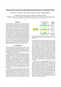
t Figure 2.1: Simple speech synthesis system based on the source-filter model for human speech production. As signal source either a series of impulses xvoi (t) – corresponding to the glottal derivative waveform – for voiced speech, or a white noise signal x uv (t) for unvoiced speech is used. The source signal is filtered by a (slowly time-varying) linear filter H(f, t) corresponding to the vocal tract filtering in speech production to yield the synthetic speech signal y(t). The coefficients for the filter H(f, t) can be determined by rule, e. g., by specification of formant frequencies and bandwidths (formant synthesis), or may be deduced from recorded speech signals by linear prediction analysis (as used for pulse-excited LP synthesis, see sect. 2.4.2). The time varying amplitude is controlled by the parameter a(t).

representation for the source signal we will shortly introduce some of them in the following. The Liljencrants-Fant (LF) model is a parametric signal model for the glottal waveform [FLL85]. The glottal waveform shape is characterized by four parameters t p , te , ta and Ee , as well as the length of the fundamental period T0 . For one fundamental period the derivative of the glottal waveform – which corresponds to the acoustic pressure signal that is used as input to the vocal tract filter – is composed of two smooth functions joined at the instant of glottal closure te . An example of the glottal waveform and its derivative represented by the Liljencrants-Fant model is given in fig. 2.2 labeled with the model parameters. The main excitation is due to the large (negative) pulse in g(t) at the instant of glottal closure t e corresponding to the delta impulses in the simplified model in fig. 2.1. Similar parameterization of the glottal waveform is used in the Rosenberg model and other related models [Ros71, Vel98]. The parameters of the above models are not all directly related to physical properties of the glottis or acoustical properties of the source signal. Thus, appropriate parameter values often have to be determined from recorded speech signals by inverse filtering (cf. sect. 4.4.1) or in an analysis-by-synthesis procedure. Although the LF model only comprises four parameters for the fundamental waveform shape it is possible to achieve a wide variety of different speech characteristics, even when the shape parameters are derived from only one control parameter [Fan95]. However, for the adequate reproduction of specific speech qualities, like source-filter interaction, or for the identification of speaker dependent variations of the fundamental waveform shape, the parameterization by the LF model does not suffice, and additional modeling effort is necessary [PCL89, PQR99]. Other parametric models represent the glottal waveform by a weighted sum of basis functions. The most common example of such a signal decomposition into basis functions is the Fourier series representation, which is also the basis for sinusoidal modeling discussed in sect. 2.4.3. The model for glottal signal generation proposed in [Sch90] and refined in [Sch92] deals

10


closing/closed phase

f(t)

open phase

tp

te te+ta T0

0 t

te te+ta

g(t)

tp

−Ee T0

0 t

Figure 2.2: Example glottal flow waveform f (t) and acoustic pressure waveform g(t) (time derivative of f (t)) generated by the Liljencrants-Fant model for one glottis cycle. Model parameters are: tp instant of maximum glottal flow, te nominal instant of glottal closure, ta time constant of exponential recovery, and Ee absolute value of glottal flow derivative at te . The periodic repetition of the signal g(t) can be used as the source signal of voiced speech instead of a series of pulses in formant synthesis (cf. fig. 2.1).

with polynomial series (Volterra shaping functions) of a sinusoidal basis function. The polynomial coefficients can be deduced from the Fourier coefficients of an inverse filtered recorded speech signal. Synthesis is performed by feeding a sinusoidal signal to a static nonlinear function. Fundamental frequency, duration, and amplitude are easily controlled by changing the respective parameters for the driving sinusoidal signal. This synthesis model allows for the generation of different spectral characteristics in the output signal by changing the amplitude and phase of the sinusoidal driving signal. For a low amplitude input signal the output signal will be almost sinusoidal. With increasing amplitude the amount of higher harmonics will increase, too. This is a feature also encountered in natural speech signals. For a fixed nonlinear function, however, the spectral characteristic of the output signal is solely determined by the amplitude and phase of the sinusoidal input signal and cannot be controlled independently of these parameters. A glottal signal generation model based on a second order resonance filter is proposed in [DA00]. Here, the nonlinear function acts on the (two-dimensional) state vector of the resonator, and its output is fed back as filter input signal. Thus, the fundamental frequency can be controlled by the resonance filter parameters whereas the waveform shape is determined by the nonlinear function. Using a quite low number of parameters the system is able to regenerate glottal flow waveforms from inverse filtered speech signals, and allows for easy control

2.4. CONCATENATIVE SYNTHESIS

11

of fundamental frequency due to the use of physically informed parameters. The approach towards the generation of the glottal signal from the field of articulatory synthesis is physical modeling of the vocal fold oscillations. Here, a simplified description of the mechanics of the vocal folds is set up by means of masses, springs, and damping elements together with equations for the fluid dynamics of the air passing through the vocal folds. The resulting differential equations are solved to yield the acoustic signal. The most prominent among physical models for the vocal folds is the two-mass model introduced in [IF72] and widely studied [Tit88, Per88, Per89, Luc93, TS97, LHVH98, JZ02], and extended, e. g., to a three-mass model in [ST95]. The main control parameter for the two-mass model is the sub-glottal pressure. To achieve a desired glottal waveform, however, a complex fine-tuning of the system parameters is necessary. However, it has been shown that, for example, by varying sub-glottal pressure and one other parameter (amount of coupling between the two model masses) a variety of possible system behaviors from nonlinear system theory is possible, like bifurcations resulting in sub-harmonics of the fundamental frequency [Luc93], and that introducing turbulence noise or random stiffness in the two-mass model induces chaotic behavior [JZ02]. If the two-mass model is directly coupled to a vocal tract model [IF72, TS97], the resulting articulatory synthesis system naturally includes feedback from the vocal tract filter to the source, which is not the case for formant or concatenative synthesis systems, in general. There is, however, no direct relation between the parameters of the two-mass model and prosodic parameters, or spectral content. Thus, as previously mentioned for articulatory synthesis in general, the control of the two-mass model in terms of F0 , amplitude, or spectral characteristics of the output signal becomes a difficult task.

2.4

Concatenative synthesis

The currently prevailing speech synthesis approach is concatenative synthesis, i. e., synthesis based on the concatenation of prerecorded speech segments. Compared to model-based speech synthesis (i. e., articulatory and formant synthesis), the use of recorded speech segments in concatenative synthesis yields a perceptually more natural synthetic speech output, as of today. Due to the use of recorded speech signals, the natural segmental quality of the signal is maintained during synthesis by concatenation to a great degree. Also, by an adequate choice for the length of the recorded signal segments the natural trajectories of signal parameters – like energy, formant frequencies and bandwidths, etc. – over time are reproduced in the synthetic speech signal. To that end, the speech signals chosen as inventory segments usually do not relate to single phonemes, but rather to transitions between phonemes, called di-phones, or even include more than two phonemes with a strong mutual influence in articulation and segmental duration (co-articulation). Strong co-articulation is, for example, encountered in the German language with its consonant clusters of various size, and here the recorded segments often comprise demi-syllables [Det83, Por94, RP98]. For concatenative synthesis with a fixed signal inventory, a medium size corpus of segments (between 1000 and 2000 segments [Por94, RP98]) has to be recorded in a controlled environment – that is, each segment embedded in a sentence at a neutral position regarding stress, lengthening, etc. The inventory segments have to be extracted from the corpus of recorded speech, which is a time-consuming task and requires considerable workload. Simple concatenative synthesis systems rely on a corpus with one instance of each segment and during the synthesis procedure the series of segments to be concatenated is chosen by rule. More elaborate concatenative synthesis systems make use of more than one instance for each inventory segment, for example stressed/unstressed instances of one segment 1 . In this case, the instance of one segment is chosen during synthesis according to the information 1

The different instances of the inventory segments may as well represent different speaking styles or different

12


about stress from text preprocessing. This is a first step towards unit selection synthesis (see sect. 2.5) and results in a concatenation of speech segments that reflect part of the natural prosody and in less artifacts due to signal manipulation and concatenation [KV98]. For natural speech synthesis we want the synthetic speech signal to resemble the trajectories of the prosodic parameters (F0 contour, segmental duration, amplitude contour) of a human speaker. Since natural prosody greatly varies with the content of the spoken message, the synthetic speech signal concatenated from the inventory segments has to be modified to achieve a desired prosody2 . This is accomplished by a suitable method to alter the prosodic parameters in the prerecorded speech segments, a prosody manipulation algorithm. Many researchers in speech synthesis consider an adequate prosody the main key for “naturalness” – in contrast to intelligibility – of synthetic speech [TL88, BHY98, KBM+ 02]. The advantage of yielding an adequate prosody, however, is of course coupled to a degradation in segmental quality when the speech signal is processed to embody the desired prosodic parameters. Or, to quote from [Bai02b]: (. . . ) the modifications are often accompanied by distortions in other spatiotemporal dimensions that do not necessarily reflect covariations observed in natural speech. In the following we present an overview of a number of prosody manipulation algorithms commonly used in current speech synthesis systems.

2.4.1

Pitch synchronous overlap add (PSOLA)

Pitch synchronous overlap add is possibly the most widely applied algorithm for prosody manipulation today. Is is based on a signal segmentation related to the individual fundamental cycles, based on estimated glottal closure instants (GCIs), and achieves fundamental frequency modification by shifting windowed signal segments from each GCI to a position in time such that the lags are the inverse of the desired fundamental frequency. The series of overlapping windowed signal segments are then added to give the modified speech signal [MC90], as depicted in fig. 2.3. Duration is altered by repeating or leaving out signal segments corresponding to individual pitch cycles in the overlap and add procedure. PSOLA is easy to implement, relies on a good estimation of glottal closure instants 3 , and can be applied to the full speech signal without any additional signal processing. However, for large scale modifications of fundamental frequency, and for duration modification of unvoiced phonemes processing artifacts are clearly audible, like artificial periodicity in unvoiced segments. In spite of the simplicity of the algorithm, the processing artifacts introduced using PSOLA for fundamental frequency modifications are not easy to describe analytically. In the original publication of the algorithm [MC90] the effect of a comb-filter (periodic spectral zeros) has been identified if the window function length is chosen four times the fundamental period, i. e., considerably longer than the usual window length of twice the fundamental period (as in fig. 2.3). This is due to the destructive interference of specific frequency components in the overlay-add process. Analysis of processed speech signals for the ‘classical’ window of length of twice the fundamental period revealed a smoothing of the formant peaks in the spectrum of the output signal, but other effects – e. g., on the phase spectrum – were described as ‘difficult to analyze’. An important prerequisite for PSOLA to avoid additional processing artifacts is emotional states of the speaker and can be chosen, e. g., according to background information about the current speech act in a dialog system [ICI+ 98]. 2 In text-to-speech systems the ‘desired prosody’ is commonly derived from the text input, either by rule or by machine learning techniques. 3 Robust estimation of the GCIs is a complex task, see [Hes83].


13

x(n)

n

... +

+

+

+

+

+

+

...

y(n)

=

n

Figure 2.3: Fundamental frequency modification using PSOLA. The original speech signal x(n) (taken from the vowel /a/, at top) is partitioned according to GCI markers (vertical lines). Segments are centered at GCIs and comprise two fundamental periods in this example. To alter fundamental frequency the windowed segments are shifted in time to positions representing GCIs according to the desired fundamental frequency contour. The shifted segments are then added to form the output signal y(n) (at bottom).

the precise and consistent determination of the GCIs, in particular the consistency of GCIs for signal parts that shall be concatenated, to avoid phase mismatches at the concatenation. Multi-band re-synthesis overlap add (MBROLA) [DL93] has been developed to overcome some of the processing artifacts of PSOLA. It applies a normalization of the fundamental period and of the glottal closure instants by harmonic re-synthesis [MQ86] of voiced segments in an off-line preprocessing stage. This normalization results in a reduction of phase mismatches in the PSOLA synthesis procedure and provides the means for spectral interpolation of voiced parts [DL93]. The MBROLA algorithm is widely used in research and experimental synthesis systems since a text-to-speech system is freely available for non-commercial use with pre-processed corpora for a variety of languages4 .

2.4.2

Linear prediction (LP) based synthesis

Linear prediction or inverse filtering (see also Chapter 4.4.1) is widely used in speech signal processing, e. g., in speech coding to reduce the bit rate, in speech analysis for formant estimation, in speech recognition for feature extraction, and also in speech synthesis. Linear prediction is related to the source-filter model of speech production in the way that the LP synthesis filter resembles the acoustic tube model of the vocal tract [MG76, sect. 4.3]. LP based concatenative synthesis uses recorded speech signals to estimate the coefficients of the LP filter for a sequence of speech frames. Frames are either of fixed length (typically about 4

http://tcts.fpms.ac.be/synthesis/mbrola.html

14


20 ms) or related to the pitch periods (pitch synchronous analysis). In the synthesis procedure the LP synthesis filter is excited either by impulses, by the residual from LP analysis, or by an artificial glottal pressure signal. Prosodic features are solely related to the excitation signal. Pulse-excited LP synthesis In pulse-excited LP synthesis, the LP synthesis filter is excited by a series of impulses. The temporal distance between two impulses determines the fundamental period T 0 and thus the fundamental frequency F0 . This resembles the simple formant synthesis model of fig. 2.1 with the filter transfer function H(f, t) determined by LP analysis. In an elaborate model also used for speech coding, the excitation consists of a series of codewords with several impulses per pitch period [CA83, CA87]. Codewords are chosen according to the LP analysis residual signal by minimizing a distortion criterion. Residual excited linear prediction (RELP) synthesis The residual from LP analysis of a speech signal is used to excite the LP synthesis filter. Without prosodic manipulations, perfect reconstruction of the speech signal is possible, only limited by a possible quantization of the residual signal for storage. For prosodic manipulations, the residual has to be processed. Commonly utilized algorithms for the prosody manipulation are LP-PSOLA and SRELP. LP-PSOLA For LP-PSOLA the PSOLA algorithm is applied to the residual signal of LP analyzed speech. Like PSOLA on the full speech signal, LP-PSOLA is performed pitch synchronously. To that means a glottis closure instant analysis (pitch marking) is necessary and also the LP analysis can be performed pitch synchronously. Fundamental frequency manipulations of voiced phonemes using PSOLA on the residual signal often result in less artifacts than for using PSOLA on the full speech signal, since for voiced speech the energy in the residual signal is commonly concentrated at the glottis closure instant. For unvoiced speech similar problems are encountered as for PSOLA applied to the full speech signal. SRELP A prosody manipulation algorithm closely related to LP-PSOLA is simple residual excited linear predictive synthesis. Here, no windowing and no overlap add procedure is applied, but the residual signal segments centered at the GCIs are simply cut or zero padded (symmetrically at both ends) to yield a segment length equal to the desired fundamental period. Since for most voiced speech signals the energy of the residual signal is concentrated at the glottis closure instants these segment length manipulations affect only little of the total signal energy. Also some of the artifacts caused by adding the overlapping signal segments in the LP-PSOLA algorithm are avoided with SRELP, however, other degradations are introduced, particularly if LP analysis results in a residual signal with the energy spread more widely over time. No frame length modifications are applied to unvoiced speech frames, avoiding the artificial periodicity artifacts encountered for such signals using PSOLA and LP-PSOLA. Like LP-PSOLA, SRELP requires GCI determination and preferably pitch synchronous LP analysis. SRELP is implemented for concatenative synthesis in the freely available Edinburgh


15

Speech Tools for the Festival speech synthesis system5 , and is also used in the phoneme-tospeech front-end for the Vienna Concept-to-Speech system6 [Kez95, Ran02].

2.4.3

Sinusoidal/harmonic-plus-noise modeling

For the sinusoidal model the speech signal is considered a sum of sinusoidal components. This relates to the model of (voiced) speech sounds being generated by a periodic source filtered by a linear vocal tract filter, both slowly time-varying. The number of sinusoidal components as well as frequency, phase, and amplitude of each component are commonly estimated frame-wise from a short-time Fourier transform or by analysis-by-synthesis of a recorded speech signal. During synthesis the signal is re-generated as the sum of the output of several sine signal generators [MQ86, Qua02]. Due to the non-stationary nature of speech, individual sinusoidal components do not only vary in amplitude and frequency over time, but new components may emerge (be born) or components may vanish (die). In the original sinusoidal model [MQ86] the sinusoidal components comprise for both the periodic and the non-periodic signal component of speech signals (the presence of these two components is most evident in mixed excitation speech sounds, like voiced fricatives or breathy vowels). As such, the sinusoidal model can only be applied for speech coding and time scale modification. The harmonic-plus-noise model [Ser89, LSM93] considers sinusoidal components with a harmonic relation, i. e., components with a frequency that is an integer multiple of the fundamental frequency, as the harmonic (periodic) signal component and the residual (difference between original speech signal and the harmonically modeled signal component) as the noise component. The residual is modeled either again by a combination of sinusoids or as a filtered time-variant random process using linear prediction and a (possibly sub-sampled) time-varying power estimate. Fundamental frequency modifications are achieved by changing the frequency of each sinusoid in the harmonically related signal component to integer multiples of the desired fundamental frequency (spectral re-sampling) [Sty01] (or by applying PSOLA to short-time synthesis frames [MC96], which, however, introduces the shortcomings of the PSOLA algorithm into sinusoidal modeling). With prosodic manipulations, the amplitudes, frequencies, and phases of the individual sinusoidal components have to be readjusted appropriately for re-synthesis to attain the correct temporal trajectories and spectral envelope. The latter can be achieved, for example, by an estimation of the spectral envelope by LP analysis and an appropriate modification of the amplitudes of the harmonic components after spectral re-sampling [WM01, Bai02b, OM02], so that the spectral distribution of the synthetic signal is maintained. For the adequate re-generation of the noise-like residual signal a pitch synchronous modulation of the random process is necessary [LSM93, SLM95, Bai02b]. To that end, the application of a parametric noise envelope for each fundamental period that is composed of a constant baseline and a triangular peak at the glottis closure instant is proposed in [SLM95]. Furthermore, the spectral content of the noise-like signal component can be shaped by an individual LP synthesis filter [SLM95, Bai02b]. Harmonic-plus-noise modeling is reported to yield synthetic speech of very high quality [SLM95, Sty01].

2.4.4

Comparison of prosody manipulation algorithms

The comparison of different prosody manipulation algorithms for concatenative synthesis is commonly performed by perceptual ratings of human subjects in terms of a mean opinion score. In [MAK+ 93], e. g., it was found that, in terms of intelligibility, LP-PSOLA and SRELP 5 6

http://www.cstr.ed.ac.uk/projects/festival/ http://www.ai.univie.ac.at/oefai/nlu/viectos/

16


perform better than PSOLA on the full speech signal, while PSOLA in turn outperforms pulseexcited LP synthesis. The harmonic-plus-noise model is also reported to give better ratings for intelligibility, naturalness, and pleasantness than PSOLA [Sty01]. In the framework of the European Cost258 action (“The Naturalness of Synthetic Speech”) an objective comparison of prosody manipulation algorithms for concatenative synthesis has been carried out [BBMR00, Bai02a].The objective rating of the prosody manipulation algorithms was based on a number of distance measures originally used for rating speech enhancement algorithms [HP98a]. A subset of these distance measures was applied to estimate the perceptual difference between natural speech samples and speech samples processed by the prosody manipulation algorithms with the task to gain the same prosody as the natural samples. As input for the prosody manipulation algorithms a natural speech sample with appropriate segmental content (same phoneme/word/sentence) but with “flat” prosody, i. e., nearly constant fundamental frequency and no stressing/accentuation/etc., was supplied. It was found that some correlation exists between the different distance measures applied, and that about 90% of total variation in the rating of the prosody manipulation algorithms is captured in the first two components from a principal component analysis. Analysis of these first two components allows to distinguish between (a) the overall distortions (signal to noise ratio, SNR), and (b) the ratio between distortions in voiced regions and distortions in unvoiced regions of the signal, and thus to rate the individual algorithms in terms of their processing quality for voiced and unvoiced speech signals, respectively. In general it was discovered that all the prosody manipulation algorithms taking part in the test could only generate signals not closer to the human target signal than a noisy reference signal with an SNR of 20 dB [Bai02a].

2.5

Unit selection

The term unit selection denotes concatenative speech synthesis with selection of the segments to be concatenated from a large database of recorded speech signals at synthesis time. The selected “units”, i. e., speech signal segments, are chosen to minimize a combination of target and concatenation (or transition) costs for a given utterance [Cam94, HB96]. The units to be concatenated can be fixed phonemic entities, for example single phonemes or syllables, or units of non-uniform size [Sag88, BBD01, PNR+ 03], which complicates the selection task considerably. The target costs are calculated by a measure of the difference between properties of a unit in the database and the target unit specified as input for the unit selection algorithm. If, for example, phonemes are considered as units, the phoneme identity, duration, mean F0 , formant frequencies, but also information about phonemic context, stress, or position in a word may be used to compute the target cost. The concatenation cost relates to the quality degradation due to joining segments with, e. g., mismatch in fundamental frequency or spectral content. A number of measures for such mismatches can be used, such as F 0 difference, log power difference, spectral or cepstral distance measures, formant frequency distances, etc. [KV98, WM98, CC99, KV01, SS01]. Minimizing the join costs is done by a path search in a state transition network (trellis) for the whole utterance with the target costs as state occupancy costs and the join costs as state transition costs (e. g., using the Viterbi algorithm) [HB96]. Since the criteria for the selection of units can be chosen for a specific purpose, unit selection may also be used to generate speech with different speaking styles or emotional content if the appropriate information is present in the database [ICI+ 98]. In many unit selection synthesis systems no or minimal signal processing for prosody manipulations or smoothing is applied, since the optimum selection of units is supposed to yield units matching the desired prosody and with reasonable small discontinuities at the concatenation points. However, particularly for proper names not incorporated in the recorded

2.6. CHALLENGES FOR SPEECH SYNTHESIS

17

database, the unit selection algorithm often has to select a series of short units with probably significant discontinuities [Stö02]. In this case, output speech quality suffers a degradation, which is especially annoying if the proper name is the segment of the utterance which carries information (like, e. g., the name of a station in a train schedule information system). Nevertheless, unit selection synthesis is very popular at current, and several experimental and commercial systems have been built, like CHATR [BT94, HB96, DC97], which, together with the Festival speech synthesis system [BTC97, BC05], forms the basis for the AT&T ‘Next-generation text-to-speech system’ [BCS+ 99].

2.6

Challenges for speech synthesis

Despite the fact that most state-of-the-art speech synthesis systems are rated well in terms of intelligibility, many systems are judged worse concerning naturalness. The possible reasons for this discrepancy seem to be numerous and are not all investigated in detail yet. In the European Cost258 action [KBM+ 02] a great effort was dedicated to the identification of reasons for this problem and to the proposition of possible remedies. As a main point for achieving natural synthetic speech the identification and reproduction of natural dynamics of the speech signal, as specified below, is considered. As noted above, for articulatory and formant synthesis the generation of adequate control parameter trajectories is a main factor determining the quality of the resulting synthetic speech signal. In data based concatenative or unit-selection synthesis this problem is partially resolved due to the utilization of recorded speech samples. Here, however, the necessary prosodic manipulations may degrade the natural signal quality. Moreover, the problem of concatenating recorded speech segments with mismatches in parameters, like spectral content, arises. For the discrimination between natural and unnatural speech signals, a main issue appears to be the dynamic evolution of the signal parameters. These parameters can roughly be classified into the categories of supra-segmental features – including prosodic parameters, like F0 trajectories and segmental duration, or formant frequency trajectories – and segmental features related to the speech waveform shape (sometimes denoted as features on the ‘signal level’) – like, e. g., spectral content, F0 or amplitude variations on a short-time level, or noise modulation. The correct (natural) evolution of both supra-segmental and segmental features over time must be considered most important for naturalness of synthetic speech, and may be responsible for the limited success of articulatory and formant synthesis – where naturalness is determined by the appropriateness of the artificially generated control parameter trajectories, in comparison to concatenative or unit selection synthesis – where, to some extent, natural trajectories are reproduced from the recorded speech signals. However, since the recorded segments may not comprise the desired prosody the rendering of natural prosodic feature trajectories is a major factor for perceived naturalness in concatenative synthesis, too. To a large part, this is a task for the so called ‘higher-level’ processing, i. e., the text or content analysis and phonetic pre-processing traditionally decoupled from the signal processing stage. Much effort has been dedicated to the generation of appropriate suprasegmental prosodic parameters, like F0 trajectories and segment durations7 from text input. However, concerning the fact that the natural segmental features are altered by the prosody manipulation algorithm, the increase in naturalness of concatenative synthesis when the ‘correct’ supra-segmental features for prosody are available to the synthesizer may be tied to a decrease in segmental quality due to (large scale) manipulations of prosodic features [JSCK03]. Nevertheless, as can already be seen from the remarks for the number of prosody manipulation algorithms above, we should aim at the target of optimizing the non-prosodic parameters, 7

Amplitude trajectories are often not modeled explicitly for concatenative synthesis.

18


too. The fact that the incorporation of the source-filter model in the form of linear prediction results in better ratings for synthetic speech quality [MAK+ 93, Sty01] already points to the importance of spectral content and precise formant frequency and bandwidth trajectories. Also the short-term variations of fundamental frequency and amplitude have long been identified as an important cue for naturalness and should be re-generated appropriately. In the setting of the harmonic-plus-noise model the importance of noise modulation is encountered again, which has been an issue in formant synthesis for quite a time. Although the decomposition into harmonic and noise parts of the speech signal seems to be adequate, their interaction must not be neglected. Recent investigations into the nature of noise modulation [JS00a, JS00b] suggest, however, that modulation by one parametric amplitude envelope (as, e. g., proposed in [SLM95]) may not suffice to adequately model noise modulation for both vowels and voiced fricatives. For unit selection synthesis the problems concerning segmental features are less significant. Especially when large units from the database can be used the natural segmental features will be simply reproduced. Here, however, and for concatenative synthesis, the problem of discontinuities at concatenation points arises. If only few concatenations of units occur the degradation of intelligibility and naturalness due to discontinuities may be negligible. For concatenative synthesis with a small inventory, however, and in specific but important cases (like, e. g., synthesis of texts including a large number of proper names) the smoothing of concatenations is of great importance for unit selection synthesis, too. At concatenation points discontinuities in the signal and of the signal phase, as well as discontinuities of fundamental frequency, spectral content, signal amplitude, etc. can occur. Particularly for synthesis with an inventory with one instance of each segment (like common diphone or demi-syllable based concatenative synthesis), pitch-synchronous processing to ensure signal phase coherence, as well as interpolation of fundamental frequency, spectral content and signal amplitude is required. In text-to-speech systems the prosody generation module commonly provides a smooth fundamental frequency trajectory, hence no additional smoothing is necessary. For LP based synthesis algorithms, spectral content can be smoothed in a straightforward way by interpolation of the LP re-synthesis filter, preferably in the log-area-ratio or line-spectral-frequency domain [Ran99, WM00]. For unit selection synthesis smooth transitions at concatenation points can be facilitated by minimizing the join costs, i. e., by selection of good matching segments. However, since join costs are not the only criterion for the selection of units there always may occur concatenation points with fundamental frequency and spectral discontinuities. If no signal processing is applied the resulting discontinuities may seriously degrade naturalness. Many discontinuities mentioned above can easily be avoided with the glottal waveform generation methods used in model-based synthesis (sect. 2.3). With these signal generation methods, on the other hand, it is often difficult to re-generate variations depending on speaker identity, speaking style, or emotional state of the speaker. Particularly in signal generation models parameterized by only a small number of parameters (like the LF model), such variations can be captured by the model only to a rather limited extent.

19

Chapter 3 Nonlinear function models For speech synthesis with the oscillator model, the correct identification of a nonlinear function f (·) ; RN → R (as will be used in sect. 4.2, eq. 4.7 on page 50) by a nonlinear function model fˆ(·) is crucial. Since the nonlinear function of the oscillator model is applied in a highdimensional space (N ≥ 3), and thus is difficult to analyze and visualize, we will examine several nonlinear function models in a one-dimensional modeling task in this chapter. The analysis shall be, however, linked to the suitability of a nonlinear function model for speech prediction and for the application in the oscillator model. The nonlinear function model should achieve a reasonably low prediction error on training and test signals. Moreover, it shall provide good generalization properties to ensure a generally stable behavior of the oscillator1 . Several attempts to speech prediction and synthesis with different realizations for the nonlinear mapping function are reported in the literature. In most cases the oscillator model has been applied to the modeling of stationary sounds, e. g., sustained vowels. Here, a large enough number of training examples is available even for nonlinear function models with a large number of parameters. Aiming at synthesis of non-stationary speech signals, the training of the nonlinear function has to be possible with speech samples on the time scale of the stationarity of the speech signal. For linear prediction, e. g., a speech signal is considered stationary on a time scale in the range of 10 to 20 ms, i. e., for only 160 to 320 samples (for a sampling rate of 16 kHz). This time scale is also the upper bound for stationarity when modeling the full speech signal by means of an stationary oscillator. To find a satisfactory nonlinear function model for a stable oscillator from a possibly small number of training data, we will account for the complexity of function models. Furthermore, the nonlinear function model shall also promote the generation of transitions between successive models over time. To this end a parameterization is preferable where the model parameters derived from different sounds are related to each other so as to, e. g., facilitate updating of the model over time and model parameter interpolation. Concerning the concept of modeling the oscillations excited by the vocal folds we have to consider that the speech signal will also consist of other excitations in general. Clearly, for unvoiced speech no excitation by vocal fold oscillations is present. For mixed excitation speech, e. g., voiced fricatives, the oscillatory signal is mingled with a strong noise-like signal component. But even for voiced speech signals like vowel signals a certain noise-like component is generally present in the speech signal. Thus, albeit we are dealing with clean signals recorded in a studio environment without ambient noise we have to make sure that the model training is robust with respect to the noise-like signal components. In the following we will examine several nonlinear function models regarding their suit1

For the meaning of “stable behavior” of the oscillator see sect. 4.2.

20

CHAPTER 3. NONLINEAR FUNCTION MODELS

ability for speech prediction and for the oscillator model. We turn our attention specifically to the generalization properties of the nonlinear function models, as well as to the possibility to train a model with low number of training data in the presence of noise. The models will be tested for regression – i. e., fitting a curve from noisy data – on the one-dimensional funcwith additive Gaussian noise, so that the model behaviors can be tion y = sinc(x) = sin(πx) πx illustrated graphically.

3.1

Radial basis function (RBF) networks

Radial basis function networks are, like multi-layer perceptrons (sect. 3.2.2), one kind of artificial neural networks (ANNs). The evolution of ANNs was inspired by the finding that the human brain computes in an entirely different way than a sequential digital computer. In an ANN complex nonlinear parallel computing takes place, and although one may doubt that an adequate model for the human brain can be built from ANNs, specific realizations of both RBF networks and multi-layer perceptrons have been proved to offer universal approximation capabilities for nonlinear functions [HSW89, HSW90, Hay94]. ANNs commonly consist of a number of similar units (neurons, processing elements) connected in the form of layers, and weights associated with the connections. The parameters of the ANN – i. e., the weights, but often also the parameters for the nonlinear functions at the units – are optimized to yield an approximation of a system function using examples of the input and corresponding output data of the system that should be modeled. A number of different algorithms for this training process are possible, depending on the network structure but also on the specific optimization criterion used. ANNs have been applied to the modeling of the nonlinear function that governs the dynamics of speech in a low-dimensional phase space embedding for speech modeling, prediction, and synthesis in [Bir95, YH95, Bir96, Kub96a, BBK97, MM99, Man99, NPC99, BMM99, MM01, CMU02a, CMU02b]. RBF networks provide a global model for a nonlinear function with good local modeling if unimodal (e. g., Gaussian) basis functions are used. In an RBF network at each unit the distance of the input vector from a center (in input space) is computed and used as input for an RBF. The network output is computed as the weighted sum of the units’ outputs. The modeling properties are influenced by the number of centers, their positions, by the shape of the basis functions (e. g., the variance for a Gaussian basis function), and by the training algorithm used to determine the network weights. The input-output relation of an RBF network is2 y = fˆRBF (x) =

Nc X i=1

wi ϕi (x) ,

RN → R ,

(3.1)

operating on a N -dimensional input vector x to compute a scalar output y, with the basis functions ϕi (·), weighting coefficients wi , and the number of basis functions and weighting coefficients Nc . The most frequently used Gaussian radial basis function is defined by ! 1 kx − ci k2 ϕi (x) = exp − , (3.2) 2 σi2 2 For other applications RBF networks often comprise an additional bias term, incorporated in the network function by using a constant ‘basis function’ ϕ0 (x) = 1 and an according weight w0 . Since speech signals in general have zero mean, we do not make use of this bias term.

3.1. RADIAL BASIS FUNCTION (RBF) NETWORKS

21

with the network center positions ci and the variances σi2 of the Gaussian basis functions. Other examples of basis functions can be found in the literature, e. g., in [Hay94]. An RBF network is a special case of kernel based function approximation with rotationally invariant kernels ϕi (x) = K(x, ci ) = K(kx − ci k). A schematic of a basic radial basis function network is depicted in fig. 3.1. w1

ϕ1 x1 x2

w2

ϕ2 w3

x x3

y(x) ϕ3

w Nc

xN ϕ Nc

Figure 3.1: Radial basis function network

The network center positions ci can be fixed a priori or depend on the training data. In the latter case the center positions are either set equal to the input training data, or a subset of the input training data, or are optimized during the training procedure (movable centers). The widths of the basis functions should be chosen in a way such that the input space is appropriately covered by basis functions. This means that the width shall be related to a maximum distance between center positions [Hay94]. For centers depending on the input data and movable centers no maximum distance can be stated a priori and the choice of basis function widths relies on heuristics. If, however, the centers are fixed – for example on an equally spaced hyper-grid (fig. 3.2 on the following page) – the influence of basis function width on the coverage of the input space by the RBF network can be exemplified as in fig. 3.3 on page 23. Here the basis function width is related to the maximum distance between adjacent network centers, which is the distance along the diagonal in the N -dimensional hyperspace √ ddiag = dgrid N , (3.3) with a spacing of the hyper-grid dgrid between centers in each dimension. The network output function for Gaussian basis functions with centers on a hyper-grid at unit intervals (d grid = 1) in the range of x ∈ [−3, 3] is calculated for unit weights. Since the centers are equally spaced the variances of the Gaussian basis functions can be chosen equal for all centers σ i2 = σg2 . The width dBF of the Gaussian basis functions shall be defined as twice the standard deviation, dBF = 2σg .

(3.4)

As can be seen a small basis function width leaves ‘gaps’ in the output for unit weights over the input region covered by the centers (fig. 3.3, left column). This results in a high prediction error for unseen data, e. g., in a cross-validation procedure. A high prediction error for a basis function width below a certain threshold has been encountered, e. g., in [Man99] for

22


x2 D

K

D

x1

ia

g

−D dd

dgrid

−D K

Figure 3.2: Two-dimensional example of RBF network centers (marked by the full circles) on equidistant hyper-grid. A number of K = 4 grid-lines are occupied by network centers. The position of the outer grid-lines D is chosen according to the maximum absolute input value. Distance between the grid-lines is dgrid = 2D/(K − 1). The √ diagonal distance between adjacent centers in the N -dimensional case is ddiag = 2D/(K − 1) N .

speech signal prediction and in [CMU02a, CMU02b] for predictions of signals from the Lorenz system. Too high a basis function width issues strongly overlapping basis functions and thus a high amount of interaction between different regions in input space. The network response for unit weights suffers a severe falloff towards the edges of the input region covered by network centers due to the missing influence from basis functions outside the input region (fig. 3.3, right column). A reasonably flat network response is obtained with a basis function width equal to the distance between adjacent network centers along the diagonal, as depicted in fig. 3.3, center column. The choice of dBF = ddiag thus seems advantageous in terms of input space coverage. Considering that the problem of gaps in input space for small basis function width is less stringent with increasing input space dimension (cf. fig. 3.3, first column) the basis function width could be chosen somewhat smaller than ddiag for higher input dimension, still providing adequate coverage. The problem of input space coverage can be relieved by normalizing the basis functions [MD89]. For Gaussian basis functions, defining 2 ik exp − 12 kx−c 2 σi (3.5) ϕi,norm (x) = N , c X 2 1 kx−cj k exp − 2 σ2 j=1

j

the output of one basis function is divided by the sum of all basis function outputs. Thus the network output for unit weights will always sum up to unity. The resulting normalized radial basis functions ϕi,norm , however, are no more rotationally invariant, i. e., no radial basis functions any more. Nevertheless, normalized radial basis function networks have been proved to be slightly superior in terms of prediction error and less sensible to the choice of basis function width compared to non-normalized RBF networks in the prediction of noisy data from a nonlinear system [CMU02a, CMU02b] and they have successfully been used for speech synthesis in [Kub96a].


N=1

N=1

dBF = 0.5 ddiag

1.4

3

1

1.2

2.5

1

0

0.6

1 0.5

0.2 -6

-4

-2

0

2

4

0

6

-6

-4

-2

x

0

2

4

0

6

N=2

dBF = 0.5 ddiag

1.2

y(x)

0.6

N=2

dBF = 1 ddiag

14

3

12

2.5

10

2

8

1.5

0.4

4

0.2

0.5

2

0

0

-2

0

2

4

6

-6

-4

-2

x N=3

N=3

dBF = 0.5 ddiag

2

4

0

6

y(x)

8 6 4 2 -2

0

2

4

0

6

-6

-4

-2

N=4

dBF = 0.5 ddiag

3 2.5 y(x)

2 1.5 1 0.5 -6

-4

-2

0 x

-4

-2

0

0

2

4

6

80 70 60 50 40 30 20 10 0

2

4

6

40 35 30 25 20 15 10 5 0

-4

-2

0 x

6

2

4

6

-6

-4

-2

0

4

6

4

6

2

x N=4

dBF = 1 ddiag

-6

4

dBF = 2 ddiag

x

y(x)

N=4

-6

N=3

10

-4

2

x

dBF = 1 ddiag

x

0

0

12

-6

0

dBF = 2 ddiag

x

y(x)

1.6 1.4 1.2 1 0.8 0.6 0.4 0.2 0

-2

6

1

-4

-4

x

3.5

1 0.8

-6

-6

x

y(x)

N=2

y(x)

1.5

0.4

0.2

dBF = 2 ddiag

2

0.8

y(x)

y(x)

y(x)

0.6 0.4

y(x)

N=1

dBF = 1 ddiag

1.2

0.8

y(x)

23

2

4

6

500 450 400 350 300 250 200 150 100 50 0

dBF = 2 ddiag

-6

-4

-2

0

2

x

Figure 3.3: Choice of basis function width. For centers on a hyper-grid with unit spacing the network output y is shown for different basis function width dBF and input space dimension N . Plotted are the network output functions of a Gaussian RBF network for unit weights (i. e., wi = 1 for all i) along one axis of input space, y(x) = y([x, 0, . . . , 0]T ) (solid line), and along the diagonal, y(x) = y([x, x, . . . , x]T ) (dashed line). Center positions are indicated by the diamonds along the x axis. In the one-dimensional case (top row) the output of the individual basis functions is overlayed (dotted lines). RBF width is parameterized with the distance√between centers along the diagonal in hyperspace, in this case of unit grid spacing ddiag = N . A small width of 0.5 ddiag results in an oscillating output (left column), especially for low dimension and along the diagonal, whereas a high width 2 ddiag results in a decay of the output function towards the edges of the input space region covered by the centers (right column). A reasonably flat response over the input space region covered by the centers is found for a width dBF = ddiag (center column).

24


To model a function given by example input-output pairs (training data) the appropriate RBF network weights wi have to be found. Rewriting the network equation as a vector product yields Nc X ˆ fRBF (x) = wi ϕi (x) = w T ϕ(x) , (3.6) i=1

with ϕ(x) = [ϕ1 (x), ϕ2 (x), . . . ϕNc (x)]T and w = [w1 , w2 , . . . wNc ]T . This equation is linear in the weights, and the solution for the unknown weights to minimize the mean squared prediction error on the training data P X (fˆ(xk ) − tk )2 , (3.7) e2 = k=1

with k = 1 . . . P , P being the number of training samples, is ˆ MMSE = (ΦT Φ)−1 ΦT t , w

with



ϕ (x ) · · ·  1 1 ..  .. Φ= . .  ϕ1 (xP ) · · ·

 ϕNc (x1 )  ..   , .  ϕNc (xP )

(3.8)

(3.9)

a P × Nc matrix composed of all basis functions outputs for all training input data vectors x1 , x2 , . . . xP , and t = [t1 , . . . , tP ]T a vector composed of the training output data (the targets). The expression on the right-hand side of eq. 3.8 contains the pseudo inverse Φ† of matrix Φ that can be computed as Φ† = (ΦT Φ)−1 ΦT if (ΦT Φ)−1 exists, i. e., if ΦT Φ is not rank-deficient. Thus, training – i. e., estimation of the weights – of a radial basis function network, with a priori fixed center positions and basis functions, is a linear problem – the weights are found by solving a system of linear equations –, in contrary to the training of other ANN realizations. The weights can be estimated in a one-step procedure and the resulting network has the best approximation property, meaning that for given input-output training examples, an RBF network with weights according to eq. 3.8 yields a better approximation of the training output data in terms of mean squared error (MSE) than with all other possible sets of network weights [PG90]3 . Generally, an RBF network achieves better prediction the higher the number of centers Nc , and yields perfect prediction at the positions of the training data for Nc = P . Here the ˆ MMSE = Φ−1 t. weights can be found using the regular inverse of the now square matrix Φ by w However, perfect prediction of the training data obviously implies over-fitting – i. e., modeling not only of the target function, but also of the concrete realization of additive noise in the training data – and thus bad noise robustness. In general, the number of training examples P should be considerably higher than the number of network parameters N c . And although a higher number of centers suggests better modeling properties for a complicated function, for the prediction of noisy chaotic signals of infinite length, RBF networks have been proved to yield optimal prediction with a finite number of network centers [LLW01]. Simulation results also suggest that with a finite number of noisy training data the optimal number of network centers can be quite low, depending on the actual data generating system. But in general an optimum number of network centers for a given task has to be searched for, e. g., by cross-validation. 3 For multi-layer perceptrons (MLP, cf. 3.2.2 on page 38) the best approximation property does not apply in general, and a training based on gradient descent has to be run several times until an appropriate model is found, because gradient descent training may merely converge to a local minimum of the error function.


25

In fig. 3.4 on the next page modeling of the sinc function by an RBF network, trained as described above, is depicted. In the noiseless case with training data covering the full range of centers (case (a)) a quite precise prediction of the target function is achieved with this network. In the noisy case (b) still a reasonably good prediction is achieved, although partial over-fitting of the noisy training data can be observed. Over-fitting is more severe in case (d), since here a smaller number of training data is used. In the case of incomplete training data (case (c) and (d), training data do not cover the full range of network centers) the network output function displays high peaks outside the training data range. This means that unreasonably large values are found for the respective network weights. This can either happen for centers that are far away from the input training data if the network tries to capture a small variation in the output training data, or if close centers receive large weights with different signs whose influence cancels at the position of the training data. This problem can be relieved using regularization where a preference for choosing small weights and a smooth function approximation is introduced (see section 3.1.2 below). The former problem can also be alleviated by pruning centers that are distant from all input training data prior to network weight learning.

3.1.1

Pruning centers distant from the training data

When training an RBF network on a speech signal embedded in phase space, often problems are encountered computing the pseudo-inverse in eq. 3.8. This is due to a high condition number, i. e., a high ratio of the largest over the smallest eigenvalue of the matrix Φ T Φ. The matrix is almost singular or rank-deficient, and instead of the inversion only a minimum norm solution can be searched for. Even if the number of training samples and thus the number of rows in Φ is increased the condition number of ΦT Φ does not significantly change for stationary vowel signals [Man99]. Taking a closer look at the situation in phase space we see that the trajectory of a stationary vowel sound only fills a small subspace of RN (cf. fig. 4.9 on page 57 or fig. 4.21 on page 73). The outputs of the basis functions corresponding to centers far away from this subspace will be close to zero for all training input data. Consequently, the corresponding columns in Φ consist of small values only. In particular, if the centers are fixed a priori and distributed over the input space, for example on a hyper-lattice, a high condition number for Φ T Φ (in the range of 1012 ) is observed. For centers located on a subset of the training input data, the condition number is somewhat lower (in the range of 109 ). However, if we want to maintain the same center positions for different speech sounds we have to deal with a set of a priori fixed centers. Here we can relieve the ill-conditioning by restricting the training process to centers in the vicinity of the actual trajectory and excluding centers far away from the trajectory from the training process. This is a simple kind of network pruning, where unnecessary parts of an ANN are removed. The effect on the network output function is exemplified in fig. 3.5 on page 27. Here the training data is limited to the interval x ∈ [−3, 3] and the RBF centers are set equally spaced in x ∈ [−5, 5]. Training the full network on the sinc function may yield large weight values for some centers outside the range of the training data due to the network trying to capture small variations of the output training data. The resulting network output function thus displays large (negative) peaks in x ∈ [−5, −3] and x ∈ [3, 5], fig. 3.5 (a). If the centers outside the training data range are pruned before network training the network output function gracefully decays to zero for test input data outside the range of training input data, fig. 3.5 (b). This kind of pruning reduces the condition number for speech signals to the range of 10 9 – the same gain as for taking network centers on a subset of the input training data. The computational load for the matrix inversion is reduced, too. One may start out with a high number of centers (several thousand) distributed in, say, the unit cube of phase space, and

26


(a)

(b) 1.2

1

1

0.8

0.8

0.6

0.6 y(x)

y(x)

1.2

0.4

0.4

0.2

0.2

0

0

-0.2

-0.2

-0.4

-6

-4

-2

0 x

2

4

-0.4

6

-6

-4

-2

1.2

1.2

1

1

0.8

0.8

0.6

0.6

0.4

0.2

0

0

-0.2

-0.2 -6

-4

-2

0 x

4

6

2

4

6

0.4

0.2

-0.4

2

(d)

y(x)

y(x)

(c)

0 x

2

4

6

-0.4

-6

-4

-2

0 x

Figure 3.4: Modeling of the sinc function by an RBF network. The RBF network has Nc = 25 centers in x ∈ [−5, 5] with Gaussian basis functions and a basis function width of dBF = 0.41 (= dgrid = ddiag , since N = 1). The sinc function is given (a) by P = 100 training samples equally spaced in x ∈ [−5, 5] without noise, (b) with additive Gaussian noise and an SNR of 10 dB, and (c) for P = 60 training samples in x ∈ [−3, 3] without noise and (d) with an SNR of 10 dB. In the plots the solid line represents the network output function, the dashed line is the target sinc function, crosses indicate the training samples in the noisy case, and the diamonds along the x axis represent network center positions. In the noiseless cases (a) and (c) the solid line (network output function) perfectly conceals the dashed line (target function) in the range of training data.

restrict the training, i. e., the matrix inversion to only a subset of the original centers (typically several hundred for speech signals). Thus, the pruning of network centers with a certain minimum distance from all input training data both relieves the problem of ill-conditioning during network training and prevents the network weights from taking unreasonably large values resulting in unwanted peaks in the network output function. If it happens that we should need the pruned centers during nonstationary synthesis, e. g., to interpolate between different sounds, we can always consider the pruned centers still present in the network with a corresponding weight value of zero. Alas, as will be shown in sect. 4.3.2, pruning does not suffice to find a good nonlinear function model for a practical (i. e., stable) oscillator, in general. A method that improves noise robustness, generalization and further reduces the condition number is regularization, described in the next section.


27

(a)

(b) 1.2

1

1

0.8

0.8

0.6

0.6 y(x)

y(x)

1.2

0.4

0.4

0.2

0.2

0

0

-0.2

-0.2

-0.4

-6

-4

-2

0 x

2

4

6

-0.4

-6

-4

-2

0 x

2

4

6

Figure 3.5: Effect of pruning distant centers of an RBF network before network training. For this example the target sinc function is provided with P = 60 training data points in the range x ∈ [−3, 3]. The RBF network is set up with Nc = 25 centers equally spaced in x ∈ [−5, 5]. (a) When training the full network some of the weights for centers outside [−3, 3] receive large values and the network output function displays large peaks, too. (b) By pruning the network centers outside [−3, 3] before network training the network output function gradually decays towards zero outside [−3, 3].

3.1.2

Regularization

The estimation of the network weights in eq. 3.8 involves the inversion of the matrix ΦT Φ. In certain cases – particularly for a priori fixed centers (see above), or if some training input data are close to others (like for almost periodic voiced speech signals) – this matrix can be ill-conditioned. If so, the estimated weights can vary considerably for small changes in the training data (e. g., by noise). The problem of system identification is said to be illposed and regularization theory should be applied [TA77]. Regularization derives a well-posed approximation of a possibly ill-posed problem and prevents the RBF model from over-fitting noisy training data [PG89]. In particular, regularization improves the modeling of noisy signals from nonlinear systems with the oscillator model in the way that the dimension of the signal and the Lyapunov exponents are reproduced better than without regularization, which is shown for the modeling of the Lorenz system in [HP98b, Ran03]. Regularization of matrix inversion Applying regularization to matrix inversion for weight estimation of an RBF network (or any other linear-in-the-weights model), the equation for the weights eq. 3.8 turns into [TA77] ˆ reg = (ΦT Φ + λI)−1 ΦT t , w

(3.10)

with λ being the regularization factor. With λ = 0 there is no regularization, increasing λ yields an increasingly well-posed problem, making the estimated values for the weights less sensitive to noise in Φ. The addition of the matrix λI ensures a full rank of the matrix that has to be inverted, thus reducing its condition number with increasing values of λ. Regularization of the network function Regularization of nonlinear function models can also be achieved by posing a constraint on the nonlinear function model fˆ(·), e. g., that it should realize a smooth function. This is achieved

28


by adding a term containing a differential operator P applied to fˆ(·) to the mean squared prediction error in eq. 3.7, yielding a cost function H[fˆ] =

P X k=1

2 (fˆ(xk ) − tk )2 + λkP fˆk ,

(3.11)

where k · k is a norm on the function space fˆ belongs to. For network centers equal to the training data (i. e., ci = xi , Nc = P ) the following linear equation for the weights [PG89] is found: (G + λI)w = t . (3.12) G is a matrix of Green’s functions applied to the input training data, Gij = G(xi , xj ). For a specific choice4 of the differential operator P the Green functions are multivariate Gaussians and an RBF network with Gaussian basis functions is obtained. The optimum weights for the network are found by solving eq. 3.12 for w with 

ϕ (x ) · · ·  1 1 ..  .. G= . .  ϕ1 (xP ) · · ·

 ϕP (x1 )  ..   , .  ϕP (xP )

(3.13)

a P × P matrix composed of the output of the Gaussians basis functions – or the Green functions – with variance σ as chosen in the differential operator P, centered at the input training data positions, i. e., ! 1 kxi − xj k2 Gij = ϕi (xj ) = exp − . (3.14) 2 σ2 Generalized radial basis functions (GRBFs) If we do not want the number of network centers Nc to be equal to the number of training samples P an extension to a number of Nc < P arbitrary RBF center positions yields the generalized radial basis function (GRBF) network [PG89], with weights ˆ GRBF = (ΦT Φ + λΦ0 )−1 ΦT t , w

(3.15)

with Φ the P × Nc matrix in eq. 3.9, and an Nc × Nc matrix composed of the output of the radial basis functions applied to the network center positions: 

ϕ (c ) · · ·  1 1 ..  .. Φ0 =  . .  ϕ1 (cNc ) · · ·

 ϕNc (c1 )  ..   . .  ϕNc (cNc )

(3.16)

Again, the amount of smoothing is determined by the regularization factor λ. For Gaussian basis functions the matrix Φ0 has all ones on the diagonal and positive values smaller than one for the off-diagonal entries. Comparing eq. 3.15 to eq. 3.10 we see that the non-zero offdiagonal entries in Φ0 make the only difference between regularization for matrix inversion and GRBFs. 4

kP fˆk2 =

R

RN

dx

P∞

m ˆ 2 σ 2m m=0 m!2m (P f (x))

with

P 2m = ∇2m , P 2m+1 = ∇∇2m , [PG89, pp. 21ff]


29

On the one hand regularization avoids over-fitting of the training data and thus improves noise robustness. On the other hand the weights are also prevented from taking unreasonably high values in regions with no training data. Figure 3.6 depicts the network output function of a regularized RBF network and regression of the sinc function. The only effect in the noiseless case (a) is an under-estimation of the function peaks since the regularization implies a preference for smaller weight values (this can and should of course be avoided by reducing regularization in the low noise cases). In the noisy cases (b) and (d), however, the effect of smoothing by regularization can be observed, cf. fig. 3.4 (b) and (d). For incomplete training data (cases (c) and (d)) regularization results in a decay of the network output function towards zero for the regions not covered by the training data. (a)

(b) 1.2

1

1

0.8

0.8

0.6

0.6 y(x)

y(x)

1.2

0.4

0.4

0.2

0.2

0

0

-0.2

-0.2

-0.4

-6

-4

-2

0 x

2

4

-0.4

6

-6

-4

-2

1.2

1.2

1

1

0.8

0.8

0.6

0.6

0.4

0.2

0

0

-0.2

-0.2 -6

-4

-2

0 x

4

6

2

4

6

0.4

0.2

-0.4

2

(d)

y(x)

y(x)

(c)

0 x

2

4

6

-0.4

-6

-4

-2

0 x

Figure 3.6: Modeling of sinc function by a regularized RBF network (eq. 3.10, λ = 1). Network parameters and all other experimental conditions are the same as in fig. 3.4 (a)-(d) on page 26. We can observe a general underestimation of target function peaks, smoothing of the network output function in the noisy case (cf. fig. 3.4, (b) and (d)), and a fast decay towards zero output for regions not covered by training data.

As we will see in sect. 4.3.2 on modeling of speech signals with the oscillator model, regularization is required to achieve stable oscillator behavior. However, the more regularization is applied the more of the detailed structure of the signal trajectories is smoothed out, and high-frequency components and cycle-to-cycle variations are no more reproduced. It is thus necessary to determine an appropriate amount of regularization, based on the nature of the signal to be modeled.

30


Cross-validation The regularization factor λ should be chosen according to the noise variance in the training data. However, the noise variance is generally not known in advance. One way to find an optimal regularization factor is cross-validation on unseen training data. For cross-validation, a part of the training data is set aside for performance validation, and the value for the unknown model parameter – in our case the regularization factor – is chosen such that it optimizes the performance, e. g., by minimizing the prediction error on the validation set. To this end, network training and validation has to be performed several times with varying regularization factors. Cross-validation is often run multiple times on different splits of the entire training data, for example in k-fold cross-validation [Sto74] by partitioning the training data set in a number of k subsets of equal size, and performing k cross-validation runs. In each run k − 1 subsets of the entire data are used for training and the remaining subset for testing. The value of the model parameter that has to be optimized can then be chosen, e. g., as the mean of the optimal values from the k cross-validation runs. In this way the drawback of cross-validation – that a part of the training data has to be set aside for validation – can be relieved. In any case, after finding the optimal parameter value, for the final network training all training data can be used. However, the value for the regularization factor is always determined using only a part of the available training data. On contrary, the two Bayesian algorithms introduced below use all available training data samples to determine the optimal regularization factor.

3.1.3

Bayesian learning of regularization factor and noise variance

In the Bayesian approach for model comparison5 and optimization of regularization [Mac92a, Mac92c, Mac92b, Nea96] the unknown parameters of a nonlinear function model, which are the network weights for our RBF network, are considered random variables. A suitable prior distribution is chosen for the probability density function (pdf) of these parameters. To that end additional hyper-parameters for the characterization of the pdfs are introduced, which are regarded as random variables, too. The optimal weight values are then chosen by maximizing the posterior pdf for the model parameters – weights and hyper-parameters – given the training data samples. In the algorithms considered here, this is achieved by an iterative procedure in the manner of the expectation-maximization (EM) algorithm [DLR77, Moo96]. Here we consider two methods applicable to an RBF network. In this section, the simultaneous estimation of the weights, the regularization factor, and the noise variance in the training data is described [Mac92a]. The next section 3.1.4 deals with a closely related training algorithm known as the relevance vector machine (RVM) [Tip01], additionally allowing for the pruning of individual network centers. Here, only a short overview of Bayesian learning is given, a more detailed derivation of the Bayesian training process for RBF networks is given in App. B. Generally, for the Bayesian approach to function model learning, we assume that the training output data are due to an additive noise model tk = f (xk ) + k ,

p() = N (0, σn2 ) ,

(3.17)

with additive zero-mean Gaussian noise samples k with variance σn2 , and the unknown nonlinear function f (·). For learning the parameters of an RBF network the function f (·) is parameterized as in eq. 3.1, i. e., we assume that the training data have been produced by 5 In [Mac92a], besides the Bayesian optimization of network parameters and regularization, the Bayesian optimization of hypothesis H (network complexity), set of basis functions A, and of the regularizer R is considered, too. Here, we restrict the description to one specific choice of H, A, and R.


31

a nonlinear function that can be parameterized as an RBF network, and additive Gaussian noise. The function parameters, in our case the network weights w, are characterized by a prior pdf. For a fixed network structure – i. e., a fixed number of basis functions, fixed centers and widths – regularization is introduced by stating a preference for small weight values, yielding smoother network functions for a given target function, by choosing the prior pdf for the weights as a zero-mean Gaussian distribution with variance α−1 : p(w|α) =

α − Nc α 2 exp − kwk2 , 2π 2

(3.18)

introducing one additional hyper-parameter α. To complete the setting for the Bayesian model, we have a second hyper-parameter which is the variance of the additive noise σ n2 [Mac92a]6 . The Bayesian choice for the network parameters is given by the values of the parameters w, α, and σn2 maximizing the posterior pdf p(w, α, σn2 |X, t): (w, α, σn2 )bay = arg max(p(w, α, σn2 |X, t)) ,

(3.19)

where X represents the collected input data vectors. The maximization of eq. 3.19 cannot be accomplished analytically, however, an efficient iterative algorithm is available. The derivation of the algorithm is detailed in App. B. The important first step to derive the iterative algorithm is a decomposition of the posterior pdf for the unknown parameters in eq. 3.19 according to p(w, α, σn2 |X, t) = p(w|X, t, α, σn2 ) p(α, σn2 |X, t) .

(3.20)

The first iteration step is the computation of the parameters of the posterior pdf for the weights from known hyper-parameters, which is the first term on the right-hand side in eq. 3.20. Due to the choice of a Gaussian prior pdf for the weights (eq. 3.18), and the assumption of additive Gaussian noise, the posterior pdf for the weights is a multivariate Gaussian distribution, too, with means µ and covariance Σ:

1 = (2π) |Σ| exp − (w − µ)T Σ −1 (w − µ) 2 −1 1 T 1 T . Σ= Φ Φ + αI µ = 2 ΣΦ t , σn σn2

p(w|X, t, α, σn2 )

− N2c

− 21

, (3.21)

The second iteration step is the update of the hyper-parameter values α and σ n2 , according to equations maximizing the second term on the right-hand side of eq. 3.20. The derivation of the update equations used below, which follows [Mac92a], is given in detail in App. B. The complete iterative algorithm for Bayesian optimization of weights and hyperparameters – and thus of regularization – is summarized by the following equations: Σ (i) = µ(i) = 6

1

ΦT Φ + α(i) I σn2 (i) 1 Σ (i) ΦT t . (i)

σn2

!−1

, (3.22)

In some references the second hyper-parameter is denoted by β, representing the inverse of the noise variance: β = σn−2 .

32


γ (i) = Nc − α(i) Trace(Σ (i) ) , α(i+1) = 1 σn2 (i+1)

=

γ (i) T

µ(i) µ(i)

,

kt − Φµ(i) k P − γ (i)

2

.

(3.23)

Here, i = 1, 2, . . . , Ni is the iteration index. For model learning the hyper-parameters are initialized with values according to the prior knowledge, i. e., some low value for α (1) corresponding to a broad prior distribution of the weights w – indicating that we do not know anything about the correct values for the weights a priori – and a ‘reasonable guess’ for the (1) noise variance σn2 . The number of iterations Ni necessary for convergence of the Bayesian learning algorithm depends on the training data. For the examples in this thesis, the iterations were stopped if both the value of the hyper-parameter α and the value of γ change less than 1% in an iteration. For the example sinc function, the iterative algorithm converges within as few as three or four iterations. The weight values maximizing their Gaussian posterior distribution are of course the means µ, and the Bayesian choice for the optimal weights thus is: ˆ bay = µ(Ni ) = (ΦT Φ + α(Ni ) σn2 w | {z λbay

(Ni )

and the resulting nonlinear function model is

}

I)−1 ΦT t ,

ˆT fˆbay (x) = w bay ϕ(x) .

(3.24)

(3.25)

ϕ(x) is the vector of basis function responses to the input vector, as in eq. 3.6. Note, that – relating to regularization by matrix inversion (eq. 3.10) – the product of the hyper-parameter values after convergence takes the role of the regularization parameter, (N ) λbay = α(Ni ) σn2 i . Thus, for an RBF network, the Bayesian optimization of the hyperparameters yields an optimization of the regularization parameter directly comparable to crossvalidation for the regularized RBF learning methods in the last section 3.1.2. Due to the probabilistic modeling, the output value y = fˆbay (x) of the RBF network (eq. 3.6) for an arbitrary input vector x can be accompanied by an estimation of the according variance σy2 (x) of the pdf for the output value y of the RBF network. The variance σy2 (x) after Bayesian learning of noise variance and regularization factor for the RBF model is [Tip01]: σy2 (x) = σn2

(Ni )

+ ϕ(x)T Σ (Ni ) ϕ(x) ,

(3.26)

using the final estimate for the noise variance σn2 and for the weights covariance matrix Σ. The standard deviation σy (x) of the predicted value y(x) represents the uncertainty of the prediction and can be visualized as error bars. Figure 3.7 on the facing page gives examples for the application of Bayesian learning to the sinc function for different amount of Gaussian noise in the training data. In table 3.1 the values estimated for the noise level and the according regularization factors are listed (also for uniformly distributed noise samples added to the training data). As can be seen the estimated noise variance is in good agreement with the correct value and the regularization imposed on the network results in a reasonably good function approximation even for low SNR. In fig. 3.8 on page 34 the network output function for incomplete training data is depicted. In this case the predicted standard deviation of the target function (indicated by the ‘error bar’ functions fˆbay (x) ± σy (x)) grows considerably for regions not covered by the training data.


33

SNR = 20dB

1.5

1.5

1

1 y(x)

y(x)

SNR = 100dB

0.5

0.5

0

0

-0.5

-0.5 -6

-4

-2

0 x

2

4

6

-6

-4

-2

1.5

1.5

1

1

0.5

0

-0.5

-0.5 -4

-2

0 x

2

4

6

-6

-4

-2

1.5

1.5

1

1

0.5

0

-0.5

-0.5 -2

0 x

0 x

2

4

6

2

4

6

0.5

0

-4

6

SNR = 0dB

y(x)

y(x)

SNR = 5dB

-6

4

0.5

0

-6

2

SNR = 10dB

y(x)

y(x)

SNR = 15dB

0 x

2

4

6

-6

-4

-2

0 x

Figure 3.7: Bayesian learning of the sinc function for different noise levels. Shown are the target function (dashed line), the network output fˆbay (x) (solid line) along with the predicted ‘error bars’ fˆbay (x) ± σy (x) (dotted lines), and the training data (crosses). The positions of network centers are indicated by the diamonds along the x axis. Network and training parameters are P = 100, Nc = 35, and Gaussian basis functions with dBF = 0.5.

34


Table 3.1: Parameters estimated by Bayesian learning of the sinc function. Training data are corrupted by additive Gaussian or uniform noise with variance σ 2 . The estimated noise variance σn2 does agree well with the actual noise variance and the amount of regularization is automatically increased with increasing noise level. The resulting network output functions for the Gaussian noise case are depicted in fig. 3.7 on the preceding page.

SNR (dB) 100

Actual noise variance σ2

Gaussian noise, estimates

Uniform noise, estimates

σn2

λ = α σn2

σn2

λ = α σn2

9.70 × 10−12

4.04 × 10−7

1.55 × 10−5

4.04 × 10−7

1.55 × 10−5

3.07 × 10−3

1.84 × 10−3

5.27 × 10−2

2.90 × 10−3

8.70 × 10−2

9.70 × 10−4

20 15

1.19 × 10−3

9.70 × 10−3

10

1.12 × 10−2

3.07 × 10−2

5

3.05 × 10−2

9.70 × 10−2

0

1.01 × 10−1

3.85 × 10−2

8.50 × 10−4

2.84 × 10−1

2.58 × 10−2

1.00 × 10−2

6.08 × 10−1

2.53 × 10−1

2.39 × 10−2

5.41 × 10−1

9.23 × 10−2

1.64

1.60

This indicates that we can not be sure whether predicted output values in these regions are correct. In general, the resulting network output function may as well display large peaks outside the region of training data, like the RBF network without regularization in fig. 3.4 (c) and (d). Pruning of centers distant from all input training data (as depicted in sect. 3.1.1 on page 25) should thus also be performed before Bayesian network training. (b)

1.2

1.2

1

1

0.8

0.8

0.6

0.6 y(x)

y(x)

(a)

0.4

0.4

0.2

0.2

0

0

-0.2

-0.2

-0.4

-6

-4

-2

0 x

2

4

6

-0.4

-6

-4

-2

0 x

2

4

6

Figure 3.8: Modeling of the sinc function with incomplete training data (x ∈ [−3, 3]) by an RBF network with Bayesian learning. (a) noiseless case, (b) noisy case with an SNR of 10 dB. Note the larger spread of the error bars fˆbay (x) ± σy (x) (dotted lines) in the regions not covered by training data.

3.1.4

The relevance vector machine (RVM)

The relevance vector machine [Tip01] is a training algorithm also based on Bayesian estimation of the RBF network weights. Again the additive noise model (eq. 3.17) is assumed as the


35

source of the training data. Deviating from the algorithm described in the previous section, an individual Gaussian prior pdf is chosen for each network weight: p(w|α) =

Nc Y i=1

p(wi |αi ) = N (0, αi−1 ) ,

p(wi |αi ) ,

(3.27)

with hyper-parameters αi , i = 1, 2, . . . , Nc , determining the variance of p(wi |αi ). A small value for αi relates to a large variance of the prior pdf for wi , which again should be the initial setting, as we do not know anything about the weights a priori. A large value for α i means that the prior pdf p(wi |αi ) as well as the posterior pdf p(wi |X, t, αi , σ22 ) for this weight is concentrated around zero. In this case, the weight wi almost certainly is close to zero. Similar to the learning process depicted in the last section, the estimation of the network weights is accomplished in an iterative procedure [Tip01], by first computing the parameters of the weights’ posterior distribution 1

Σ (i) = µ(i) = (i)

σn2 (i) 1 σn2 (i)

ΦT Φ + A(i)

!−1

,

Σ (i) ΦT t ,

(3.28)

(i)

(i)

with A(i) = diag([α1 , α2 , . . . αN ]). Again, small values for the initial values of the hyper(1) parameters αk are chosen (i. e., a flat prior distribution for the weights is assumed), and after evaluating eq. 3.28 the hyper-parameters are updated according to (i+1)

αk

(i)

=

γk

(i) (µk )2

k = 1 . . . Nc(i) ,

, 2

1 σn2 (i+1) (i)

=

kt − Φµ(i) k P (i) , N c − k γk (i)

(i)

γk = 1 − αk Σkk ,

with k = 1 . . . Nc(i) .

(3.29)

Again, i = 1, 2, . . . , Ni is the iteration index, µk is the k th element of the mean vector µ, Σkk is the k th element on the diagonal of the covariance matrix Σ, and γk are additional intermediate parameters equivalent to γ in eq. 3.23. While iterating eqs. 3.28 and 3.29 some αi tend to ∞, meaning the pdf of the corresponding weight is concentrated around zero and so the corresponding basis function can be pruned without impairing network performance. Iterations are continued with the corresponding (i) values µi removed from µ, the according rows and columns deleted from Σ and with N c reduced by the number of pruned basis functions. In our implementation of the RVM training process iterations are stopped if the number of centers does not change during 10 iterations. After the iteration the weights for the remaining centers are set to the mean values of their posterior pdf: ˆ RVM = µ(Ni ) . w (3.30) The nonlinear function model provided by the RVM is 0 ˆT fˆRVM (x) = w RVM ϕ (x) , (N )

(3.31)

ˆ RVM the Nc i -dimensional vector of weights remaining in the network after Ni iterawith w tions, and ϕ0 (x) the vector of the remaining basis function’s responses to the input vector.

36


The RVM thus represents the nonlinear function by a sparse RBF network, comparable to support vector machines [Vap95]. Only centers that are relevant to the modeling of a function are used for regression7 . Error bars for the predicted output values can be computed by the same formula as for the Bayesian training (eq. 3.26 on page 32), with the vector ϕ(x) and the matrix Σ now only containing values corresponding to the centers not pruned during RVM training iterations. In fig. 3.9 on the facing page, the modeling of the sinc function by the RVM is depicted (cf. also [Tip01]). In the first four subplots (a)-(d) the same network and training parameters as for the previous modeling tests (see caption of fig. 3.4 on page 26) were used. Here we observe that in the noiseless cases (a) and (c) nearly all of the network centers are used for the RVM regression. In the noisy case (b) and (d), somewhat more of the centers are pruned. For incomplete training data (case (c) and (d)) also the outlying centers are used for the regression and the problem of large weight values and peaks in the network output function (cf. fig. 3.4 on page 26) persists. For the choice of a larger basis function width, fig. 3.9 (e)-(h), a larger number of basis functions are pruned, due to the higher interaction between basis functions for different centers. Outlying centers, however, are still included in the final RVM. This calls for a priori pruning of centers distant from the training input data for the RVM, or for the use of network centers equal to (a subset of) the input training data as described in [Tip01]. The regression behavior of the RVM on the sinc function generally resembles the behavior of the RBF network with Bayesian learning of regularization factor and noise variance, with the exception that for a large enough basis function width the smooth target function is represented by a smaller number of basis functions.

3.2

Other models

We will give a very brief overview of other realizations of the nonlinear function that have also been used for the oscillator model or closely related models.

3.2.1

Locally constant (nearest neighbor) approximation

A straightforward approach to modeling the nonlinear function is the construction of a locally constant approximation based on the training data [KK94]. The function f (x) is approximated by a piecewise constant function with the function value corresponding to the output target of the nearest training sample in input space: y = fˆloc (x) = ti ,

i = arg mink=1...P (kx − xk k) ,

RN → R ,

(3.32)

with x the N -dimensional input vector, xk , k = 1 . . . P the input vectors of the training qP data, N 2 and tk the corresponding outputs (targets), the vector norm is the Euclidean kxk = i=1 xi . The arg min function picks the index k that minimizes its argument. Thus, the dynamics in phase space are represented by a number of vectors each corresponding to a certain region of phase space and the respective outputs. Predictions are made by finding the appropriate prototype vector for the region containing the current input vector and returning the corresponding output value. In fig. 3.10 on page 38, the manner a locally constant model approximates the sinc function is exemplified. The output function is piecewise constant, and if enough training samples are available a reasonably good approximation of a given function can be achieved (fig. 3.10 (a)). For noisy training data (fig. 3.10 (b)) the noise is preserved by the locally constant model, and 7

RVM learning can also be applied for minimizing the number of filter taps in adaptive filters [KKP03].

3.2. OTHER MODELS

37

(a)

(b) 1.2

1

1

0.8

0.8

0.6

0.6 y(x)

y(x)

1.2

0.4 0.2

0.4 0.2

0

0

-0.2

-0.2

-0.4

-0.4 -6

-4

-2

0 x

2

4

6

-6

-4

-2

1.2

1.2

1

1

0.8

0.8

0.6

0.6

0.4 0.2

6

2

4

6

2

4

6

2

4

6

0.2 0

-0.2

-0.2 -0.4 -6

-4

-2

0 x

2

4

6

-6

-4

-2

(e)

0 x

(f)

1.2

1.2

1

1

0.8

0.8

0.6

0.6 y(x)

y(x)

4

0.4

0

-0.4

0.4

0.4

0.2

0.2

0

0

-0.2

-0.2

-0.4

-0.4 -6

-4

-2

0 x

2

4

6

-6

-4

-2

(g)

0 x

(h)

1.2

1.2

1

1

0.8

0.8

0.6

0.6 y(x)

y(x)

2

(d)

y(x)

y(x)

(c)

0 x

0.4 0.2

0.4 0.2

0

0

-0.2

-0.2

-0.4

-0.4 -6

-4

-2

0 x

2

4

6

-6

-4

-2

0 x

Figure 3.9: RVM modeling of sinc function. The centers finally used by the RVM are indicated by the diamonds on the x axis. Network parameters for case (a)-(d) are the same as given for fig. 3.4 on page 26, for case (e)-(h) the width of basis functions is doubled. The network output function (solid line) is accompanied by the ‘error bars’ calculated in eq. 3.26 (dotted lines). The number of centers is reduced more if the width of the basis function is chosen larger. In the case of training data not covering the range of centers (cases (c), (d), (g), and (h)), some outlying centers are not eliminated in the training procedure and large weights are assigned occasionally, resulting in peaks in the network output function.

38


within the range of training input data the function model will reproduce a similar amount of noise in the output as is present in the training data. This may constitute a drawback in terms of generalization. However, it is advantageous if we want the oscillator model to reproduce both voiced and unvoiced excitation. For incomplete training data (fig. 3.10 (c) and (d)) the locally constant model implicitly does a constant extrapolation to regions not covered by the training data. (b)

1.2

1.2

1

1

0.8

0.8

0.6

0.6 y(x)

y(x)

(a)

0.4

0.4

0.2

0.2

0

0

-0.2

-0.2

-0.4

-6

-4

-2

0 x

2

4

-0.4

6

-6

-4

-2

1.2

1.2

1

1

0.8

0.8

0.6

0.6

0.4 0.2

4

6

2

4

6

0.4 0.2

0

0

-0.2

-0.2

-0.4

2

(d)

y(x)

y(x)

(c)

0 x

-6

-4

-2

0 x

2

4

6

-0.4

-6

-4

-2

0 x

Figure 3.10: Example of function approximation by the locally constant model. Modeling of the sinc function a) using 100 training samples in the range x ∈ [−5, 5] without noise, b) with an SNR of 10dB, and c) using 60 training data samples in x ∈ [−3, 3] without noise and (d) with an SNR of 10dB.

Using a recorded speech signal for model learning, the approximation of f (·) is constructed from the state transitions in phase space observed for the speech signal. These transitions are, e. g., stored in a codebook and for synthesis the nearest neighbor of the current state in the codebook is accessed for prediction. The locally constant model with a frame-wise adaptive codebook has been used for time scale modification of speech signals [KK94].

3.2.2

Multi-layer perceptrons

Multi-layer perceptrons (MLPs) are ANNs more closely related to biological functions in the brain than RBFs. At the nodes of the network a nonlinear function related to the threshold for firing of a neuron (activation function) is applied to a weighted sum of the previous nodes’

3.2. OTHER MODELS

39

outputs. A fully connected MLP with scalar output is defined by the equation   !  Nl−1 Nl N1 X X X l−1 1 Wk,j x k  . Wj,i . . . g1 wil gl−1  y = fˆMLP (x) = gl  i=1

j=1

(3.33)

k=1

Here, l is the number of network layers, Nm the number of units in layer m, the matrices m ] and the vector w l = [w l ] are the weights at the connections from unit i in layer W m = [Wj,i i m − 1 to unit j in layer m, and gm (a) is the activation function at the units of layer m. An activation function often used is g(x) =

2 −1 , 1 + exp(−2cx)

c>0 ,

(3.34)

which resembles a threshold function for c → ∞, but is continuous and differentiable, which is essential for MLP training. The network parameters are the weights between network layers W m , m = 1, . . . l − 1 and wl , the parameter(s) of the activation functions, and commonly also a bias vector for each layer to shift the individual activation functions along the input axis. MLPs with as few as two layers and smooth activation functions are capable of approximating an arbitrary function (MLPs are said to be universal function approximators) [HSW89, HSW90]. There is, however, no constructive rule to determine the structure and size of an MLP to achieve a certain amount of approximation accuracy. Training of the MLP parameters has to be performed in an iterative procedure, the most commonly used training algorithm is back-propagation [Hay94]. Here, the search for the optimal network parameters is performed by gradient descent on the error function surface, with random initialization of the parameters. Thus, the solution finally found may only represent a local minimum of the error function instead of the desirable global minimum. Commonly, the training process is performed for several parameter initializations and the network with minimum error will be used. In fig. 3.11 on the following page again the regression for the sinc function is depicted. For these examples, the training process had to be performed several times until an MLP with a reasonably low modeling error was found. One can see that both in the noiseless cases (a) and (c) and for additive noise (b) and (d) the network function reasonably well fits the original function. With incomplete training data (c) and (d), though, the network output function tends to large (negative) values for |x| > 3 . This does not happen for all training runs, though, so one can manually choose a network with a suitable network output function for incomplete training data. Moreover, the network output is always limited by the maximum of the activation function in the output layer. However, the output of an MLP may basically display arbitrary output (in the range allowed by the output activation function) for an input in regions not covered by the input training data due to the lack of an error criterion for these regions. The transition and interpolation between different models (e. g., for different speech sounds) using MLPs is hindered by the missing relation between MLP parameters for different models. Even for the same training data, an MLP model may internally be represented by completely different parameterizations. Due to the usually identical activation functions in one layer, and due to the full interconnection matrix between the layers, the Nm units in layer m can be permuted ad libitum, so there is no clear ordering of one layer’s units. Moreover, different initializations of the network parameters may result in equal solutions in terms of prediction error (at local minima of the error function) with completely different parameter values. Thus, non-stationary synthesis (e. g., transitions between different phonemes) may only be performed by switching between different nonlinear function models.

40


(a)

(b) 1.2

1

1

0.8

0.8

0.6

0.6 y(x)

y(x)

1.2

0.4

0.4

0.2

0.2

0

0

-0.2

-0.2

-0.4

-6

-4

-2

0 x

2

4

-0.4

6

-6

-4

-2

1.2

1.2

1

1

0.8

0.8

0.6

0.6

0.4

0.2

0

0

-0.2

-0.2 -6

-4

-2

0 x

4

6

2

4

6

0.4

0.2

-0.4

2

(d)

y(x)

y(x)

(c)

0 x

2

4

6

-0.4

-6

-4

-2

0 x

Figure 3.11: Example of function approximation of the sinc function by a multi-layer perceptron, (a) using 100 training samples in the range x ∈ [−5, 5] without noise, (b) with an SNR of 10 dB, (c) using 60 training data samples in x ∈ [−3, 3] without noise, and (d) with an SNR of 10 dB. Again, dashed lines show the target function, solid lines the network output function, and crosses the training examples in the noisy cases. The MLP architecture is 1-9-1 (input, hidden, output units) resulting in 28 network parameters, and g i (·) = tanh(·). Network training has been performed using the Levenberg-Marquardt back-propagation algorithm limited to 30 epochs. The network was trained with several different initializations and examples with “good” approximation properties are depicted here.

3.2.3

Multivariate adaptive regression splines (MARS)

Another approximation for a nonlinear function are multivariate adaptive regression splines [Fri91], which have been used for nonlinear sub-band synthesis of speech [HK98]. Here, the input space is repeatedly partitioned and each sub-region is approximated by a product of linear spline function. The partitioning threshold is adapted to minimize the squared error in each stage. During the repeated partitioning the spline functions from earlier stages are used as basis for the next approximation step (up to a specified number of maximum interaction). Function approximation by MARS results in a continuous output function, consisting of products of linear spline functions in the components of the input vector for each of the final partitions of input space. The one-dimensional example for the sinc function is depicted in fig. 3.12. If a high enough number of splines is used the target function is approximated well (fig. 3.12 (a)). In the presence of noise the MARS model still captures the general picture (fig. 3.12 (b)), suggesting good noise robustness. For the case of incomplete training data (fig. 3.12 (c),(d)) the modeling by linear splines results in a linear extrapolation for regions

3.3. CONCLUSION

41

not covered by the input training data. Thus, the absolute value of the model output may attain large values for an input outside the training data, especially if the maximum absolute output value in the training set is reached at the border of the region of input training data. (b)

1.2

1.2

1

1

0.8

0.8

0.6

0.6 y(x)

y(x)

(a)

0.4

0.4

0.2

0.2

0

0

-0.2

-0.2

-0.4

-6

-4

-2

0 x

2

4

-0.4

6

-6

-4

-2

1.2

1.2

1

1

0.8

0.8

0.6

0.6

0.4 0.2

4

6

2

4

6

0.4 0.2

0

0

-0.2

-0.2

-0.4

2

(d)

y(x)

y(x)

(c)

0 x

-6

-4

-2

0 x

2

4

6

-0.4

-6

-4

-2

0 x

Figure 3.12: Regression of the sinc function by a MARS model. The training was limited to a maximum interaction level of 3 and a maximum number of basis functions equal to 20. As in the previous examples, case (a) is for 100 training samples in x ∈ [−5, 5] without noise, case (b) with additive Gaussian noise with an SNR of 10 dB, and case (c) for 60 training samples limited to x ∈ [−3, 3] without noise and (d) with an SNR of 10 dB.

Due to the adaptive partitioning depending on the training data, the partitioning thresholds and spline coefficients will be different for different target functions and training data. A direct relation between MARS models for different sound signals can thus not be easily established.

3.3

Conclusion

In this section a number of candidate models for the nonlinear function in the oscillator model were presented and tested in a simple one-dimensional regression task with noisy and incomplete training data. The aim was to test their usability for the oscillator model, and to find the reasons for some of the problems that are reported in the literature and became apparent in our work. The most commonly used indicator for a “good” nonlinear function model is the modeling error. A summary of the modeling errors of the candidate models with approximately the same number of parameters for the sinc function is given in table 3.2. Here we can see that

42


the best performance, i. e., the lowest prediction error is achieved by models using continuously differentiable functions, namely the RBF and MLP networks, on the noiseless training data. The worse performance of the locally constant model and the MARS model on noiseless training data is due to the function approximation by a finite number of constant or linear splines, respectively. In the case of noisy training data, the locally constant model displays a modeling error in the range of the noise level in the training data, i. e., the locally constant model preserves the noise of the training data (see also fig. 3.10 on page 38), whereas – for the reasonably large number of training data in the examples – all other models suppress the noise to some extent. Table 3.2: Modeling error for regression of the sinc function of candidate nonlinear function models for different amount of Gaussian noise in the training data. The numbers are associated with the conditions reported in the plots in the last sections, for complete training data (100 samples for x ∈ [−5, 5]). The modeling error is computed for the noiseless target sinc function for 500 points in x ∈ [−5, 5] and normalized relative to the signal level.

SNR of training data ∞

20 dB

10 dB

Model

Relative modeling error (dB)

RBF network without regularization

−55.29

−25.85

−15.83

RBF, reg. matrix inversion (λ = 1)

−22.11

−21.72

−17.43

GRBF (λ = 1)

−18.54

−18.67

−16.35

RBF, cross-validation

−55.34

−26.85

−15.62

(λ = 10−3 )

(λ = 0.1)

(λ = 1)

−55.29

−26.29

−16.99

(λ = 1.6 × 10−5 )

(λ = 1.8 × 10−2 )

(λ = 0.14)

RVM

−55.18

−26.10

−16.46

Locally constant (nearest neighbor)

−25.76

−19.94

−10.93

MLP, backprop.

−27.38

−19.91

−15.82

MARS

−20.65

−19.84

−14.48

Bayesian RBF

The basic RBF network, the regularized RBF network with cross-validation, Bayesian learning, as well as the RVM perform similarly in terms of modeling error, with a very good function approximation in the absence of noise and a modeling error about 6 dB below the noise level in presence of noise in the training data. The regularized RBF network with a fixed regularization factor λ = 1 exhibits an almost constant modeling error, regardless of the noise level, both for regularization of matrix inversion and GRBFs. This is primarily due to the preference of lower weight values induced by regularization, which leads to a general underestimation of function peaks (cf. fig. 3.6 on page 29). When using cross-validation or the Bayesian algorithm to determine the regularization factor less regularization is applied in the lower noise cases, leading to a better function approximation. However, the ratings of the different function models in terms of modeling error may not

3.3. CONCLUSION

43

be sufficient to prove the suitability for use in the oscillator model [HP98b, CMU02a]. For other preconditions it is not easy to give quantitative measures. We will, however, try to give some qualitative criteria here. As we have previously noted the training data for speech signals in a multi-dimensional phase-space embedding may only fill a small region of phase space. So, we have to deal with incomplete training data during nonlinear function training. To explore the suitability of the candidate models for such a task we have restricted the training process for modeling the sinc function to a limited region of the input variable x ∈ [−3, 3] and observed the model output function for x ∈ [−5, 5]. Generally, all model output functions for regression in x ∈ [−3, 3] resemble the results stated above. However, for inputs outside the region of training data, different behavior is observed. The locally constant model results in a constant extrapolation of the output value corresponding to the nearest training input value (fig. 3.10 on page 38 (c)). This can be considered favorable for the use in the oscillator model since the nonlinear function output cannot grow beyond the range of training output data and an arbitrary state in phase space should quickly converge to the region of the actual signal trajectory during synthesis. For the basic RBF network with fixed centers on a hyper-grid it was observed (fig. 3.4 (c)) that the network output function may display large peaks in the region not covered by the training data, due to the assignment of large weights to the corresponding centers. This problem could be relieved either by restricting the center positions to the region in input space covered by the training data (sect. 3.1.1) or by regularization (sect. 3.1.2). In both cases the network output function decays to zero output outside the training data region. When applied in the oscillator model this means that, for each state outside the training data, the system trajectory would be pulled to the origin. This seems problematic if the origin of state space itself is not covered by the training data. However, if basis functions with infinite support (like Gaussians) are used, the system trajectory will also approach the original trajectory, even if the origin is not near to the training data (cf. [Man99]). By preventing high peaks in the network output function we shall also prevent an oscillator behavior with large amplitude intermediate pulses as observed in [Man99, fig. 6.11] for the RBF network without regularization (cf. sect. 4.3.2). The Bayesian RBF network and the relevance vector machine may, similarly to the RBF network without regularization, assign large weight values to centers away from the input training data, especially in the case of noiseless training data when regularization is automatically reduced (e. g., fig. 3.9 on page 37, subplot (c)). Thus, the center positions for the Bayesian network training should be restrained to the input space region covered by the training data, either by choosing the centers equal to (a subset of) the training data as in [Tip01] or by pruning centers away from the training data before network training. For the MLP the network output function may attain arbitrary values in the range of the activation function in the output layer for regions not covered by the training data. The MARS model may assign splines with nonzero slope at the borders of regions covered by training data. Thus, both have to be considered dangerous to the stability of the oscillator model. Using a relatively small number of training data examples as compared to the number of nonlinear function parameters – like in the examples 100 or 60 training samples compared to about 30 parameters8 – we have to consider the problem of over-fitting noisy training data and of bad generalization. As we have seen this might be a concern for the basic RBF network. However, both a priori pruning, and thereby reducing the number of network parameters, and regularization mitigates this problem for smooth target functions. Also the MLP and the MARS model can be considered to give good interpolation of a smooth target function in the noisy case. 8

With the exception of the locally constant model, which uses all training samples as ‘parameters’.

44


Concerning the aim of associating a sequence of nonlinear function models for different sounds (different training data), only the RBF model with a priori fixed centers and basis function widths can provide such relations. Here a clear correspondence between the weights for different training data is given according to the position of the RBF centers in input space. This correspondence can also be retained if different centers are pruned for different training data in the RVM, by assigning zero weight values to the pruned centers. To conclude, for the realization of the nonlinear function in the oscillator model, the RBF network with a priori fixed center positions and basis functions widths seems to be the favorable choice. We will apply pruning of network centers that are more than a specific maximum distance away from all input training data to ensure a good numerical conditioning for matrix inversion during training, and to prevent peaks in the network output function. Furthermore, we will use regularization to further promote good generalization and robustness of the network output function for noisy training data. We will, in particular, make use of automatic determination of the regularization factor, by cross-validation or Bayesian learning of the noise variance and regularization factor.

45

Chapter 4 Speech synthesis with the oscillator model In this chapter we examine modeling and re-synthesis of speech signals by a nonlinear oscillator. The oscillator model used in our work is based on a nonlinear predictor for time series. In sect. 4.1 we present considerations for optimal time series prediction. The oscillator model is introduced in sect. 4.2. In sect. 4.3 we examine the application of the oscillator model using the various nonlinear function models presented in Chapter 3 to stationary full speech signals. In sect. 4.4 we argue for combining linear prediction and the oscillator model to achieve a higher number of successfully re-synthesized signals. Finally, in sect. 4.5 we present some examples how to generate speech signals with varying fundamental frequency and transitions between different speech sounds by model interpolation.

4.1

Time series prediction

Prediction of scalar time series {x(n)} refers to the task of finding an estimate x ˆ(n + 1) of the next sample x(n + 1) based on the knowledge of the history of the time series, i. e., the samples x(n), x(n − 1), . . .. A common approach is linear prediction [MG76], where the estimate is based on a linear combination of NLP past samples x ˆLP (n + 1) =

NX LP −1 i=0

ai x(n − i) ,

(4.1)

with the prediction coefficients ai , i = 0, . . . , NLP −1. The linear prediction approach, however, does not account for nonlinear dependencies in the time series. Introducing a general nonlinear function f (·) : RN → R applied to the vector x(n) = [x(n), x(n − M ), . . . , x(n − (N − 1)M )]T

(4.2)

of past samples, we arrive at the nonlinear prediction approach x ˆNP (n + 1) = f (x(n)) .

(4.3)

The vector series {x(n)} is called an time-delay embedding of the system underlying the time series {x(n)} in N -dimensional space. Here we already include the option of using a vector x(n) of non-contiguous past samples (instead of the latest N samples [x(n), x(n−1), . . . , x(n−(N − 1))]T ) from the original time series in the embedding by introducing an embedding delay M that can be chosen M ≥ 1. The choice of M > 1 has the advantage of increased memory length (number of past samples in the delay line) for a fixed embedding dimension (which relates to complexity of the nonlinear function model, see below). A schematic of this nonlinear predictor is given in fig. 4.1.

46

CHAPTER 4. SPEECH SYNTHESIS WITH THE OSCILLATOR MODEL

x ˆ(n + 1) xe (n + 1) f (x(n))

− M

M x(n)

x(n + 1)

Figure 4.1: Nonlinear predictor for scalar time series

4.1.1

Embedding dimension

The choice of embedding dimension N , i. e., the dimension of the embedding vector x(n), is based on either the dimension of the original system that gave rise to the signal (which is often unknown) or on an estimate of the – possibly fractal – dimension of the attractor on which the signal evolves. The dimension of the embedding determines the dimension of the input space of the prediction function f (·) in our oscillator, and thus is most often related to the complexity of the nonlinear function model for f (·). Furthermore, the higher the dimension of the input space for a parametric nonlinear function model is, the more sparsely this input space will be filled with training data: This is known as the so-called “curse of dimensionality”. Hence, the lowest possible embedding dimension should be searched for. An embedding theorem going back to [Whi36] says, that a d-dimensional smooth manifold has a diffeomorphism in R2d+1 generated by a ‘generic smooth map’. Thus, almost any ddimensional manifold can be embedded in another space of dimension N = 2d + 1 by an invertible (i. e., one-to-one) mapping. For dynamical systems with only a scalar observable (like a speech signal), Takens [Tak81] proved an analogous theorem for the system attractor generated by a time-delay embedding (eq. 4.2). According to Takens’ theorem the attractor dynamics of the original nonlinear system that gave rise to a scalar time series can be fully reconstructed from a time-delay embedding (eq. 4.2) if the embedding dimension is N ≥ 2d + 1 ,

(4.4)

depending on the dimension d of a manifold that can hold the attractor of the observed signal, i. e., d being an integer larger than the fractal dimension df of the observed signal attractor. This embedding theorem is valid even for a chaotic system. Thus, we can always embed a signal with a fractal dimension of, e. g., df = 2.1 in a time-delay phase space of dimension N ≥ 2 · d2.1e + 1 = 7, regardless of the actual dimension of the system state vector that gave rise to the signal (which may be dorig = 100). Takens’ theorem is valid for arbitrary embedding delay M , noise-free observations of the steady state attractor, and if the time series is observed over an infinite time interval. A little more relaxed is the embedding theorem by Sauer et al. [SYC91]. The steady-state attractor of an unknown dynamical system can be fully reconstructed in an N -dimensional embedding if N > 2 df , (4.5) with df being the fractal dimension of the attractor. According to this theorem, an embedding dimension of N = d2 · 2.1e = 5 suffices for a signal with fractal dimension df = 2.1.

4.1. TIME SERIES PREDICTION

47

The fractal dimension can be estimated indirectly from an observed scalar time series, e. g., using the box-counting dimension or correlation dimension for the attractor observed in an embedding phase space [ABST93]. However, some definitions for the fractal dimension, like the Hausdorff dimension may not be used with this embedding theorem [SYC91]. For voiced speech signals a correlation dimension of between one and two has been found in [BK91], values below three in [Tow91, BM94], but also higher values up to four have been stated in the literature. This means an embedding dimension N between three and nine will be necessary for the reconstructed phase space to represent the dynamics of a voiced speech signal. However, in [BK91] a saturation of the redundancy of the state space embedding with optimized embedding delay (see sect. 4.1.2 on the next page) for sustained vowel signals at all dimensions N ≥ 3 has been found, indicating that a reconstruction dimension of three suffices for these signals if the embedding delay is chosen appropriately. For the application of the oscillator model with a locally constant nonlinear function model [KK94], it has been found that stationary speech can be reproduced well by a low-dimensional embedding N = 4, but for transient signals a higher embedding dimension is necessary. In general, the above embedding theorems ensure a reconstruction of the original system dynamics, and they are sufficient, but not necessary conditions [HP98b], meaning that a suitable choice of the embedding delay M may allow to reconstruct a signal in a phase space of a lower dimension N than the embedding theorems require. A way to find a sufficient embedding dimension, if the embedding delay M is chosen already, is to look at the number of false neighbors for the points x(n) on the trajectory in phase space [KBA92]. A false neighbor is a nearby point x(k), kx(k) − x(n)k < whose trajectory significantly diverges from the trajectory of x(n). Increasing the embedding dimension N the number of false neighbors for a low-dimensional signal gets lower and should reach a minimum at the dimension which is sufficient for the embedding. In fig. 4.2 the fraction of false neighbors for some sustained vowel signals from male and female speakers are plotted as a function of N . As we see the number of false neighbors is close to zero for all signals for N ≥ 4, suggesting that an embedding dimension of N = 4 suffices for sustained vowel signals.

Male vowel /a/, vowel /e/, vowel /E/, vowel /E/, vowel /i/, vowel /i/, vowel /o/, vowel /u/, vowel /ø/, vowel /Y/,

0.9 Fraction of false neighbors

Female

0.8 0.7 0.6 0.5

speaker speaker speaker speaker speaker speaker speaker speaker speaker speaker

1

8 7 1 6 1 8 1 6 7 3

0.4 0.3 0.2 0.1 0

vowel /e/, vowel /i/, vowel /o/, vowel /u/, vowel /ø/,

0.9 Fraction of false neighbors

1

0.8 0.7

speaker speaker speaker speaker speaker

5 1 4 1 1

0.6 0.5 0.4 0.3 0.2 0.1

1

2

3

4 N

5

6

7

0

1

2

3

4

5

6

N

Figure 4.2: Fraction of false neighbors as a function of embedding dimension N for sustained vowel signals from male and female speakers. Embedding delay was chosen M = 13 for male, and M = 11 for female speakers (at a sampling rate of fs = 16 kHz). The number of false neighbors is calculated by the function false nearest from the nonlinear time series analysis package TISEAN [HKS99].

7

48


4.1.2

Embedding delay

The choice of embedding delay M should be guided by properties of the time series, too. The samples in x(n) should be chosen so as to serve as independent coordinates in reconstruction space. The choice of M > 1 prevents the usage of adjacent, and thus possibly highly correlated samples from the time series in the embedding. If, however, M is taken too large, the samples x(n) and x(n − M ) will be disconnected, or statistically independent, especially for chaotic time series. Also, for time series with harmonic components, the embedding delay should be smaller than half the fundamental period [SYC91]. The choice of an appropriate intermediate value for M to yield uncorrelated samples in x(n) can be based on the auto-correlation function, e. g., by choosing M equal to the time lag of the first zero crossing of the auto-correlation, thus yielding linearly uncorrelated samples in x(n) and x(n − M ). Minimizing linear dependence, however, might not be optimal, in particular for the embedding of signals coming from nonlinear systems (cf. [Ber97, App. B]). A better way is to look at the mutual information (MI) between the samples in two time series {x(n)} and {x(n − L)} as a function of lag L and to choose the embedding delay M at the lag L at which the first minimum of the mutual information occurs [Fra89, Ber98]. For sustained vowel signals the first minimum of the mutual information typically occurs for a delay between 0.5 and 1 ms (i. e., for a lag L between 8 and 16 samples at 16 kHz sampling rate). Mutual information as a function of delay is depicted for a number of sustained vowel signals spoken by male and female speakers taken from the speech signal database used to test our model (see sect. 4.3) in fig. 4.3. In several cases the ‘first minimum’ is not very pronounced. It is, however, clear that a choice of M > 1 is advantageous in any case. Male vowel /a/, vowel /e/, vowel /E/, vowel /E/, vowel /i/, vowel /i/, vowel /o/, vowel /u/, vowel /ø/, vowel /Y/,

2.5 2 MI (nats)

Female

1.5

speaker speaker speaker speaker speaker speaker speaker speaker speaker speaker

3

8 7 1 6 1 8 1 6 7 3

0.5

0.5

5

10

15 L (samples)

20

25

5 1 4 1 1

1.5 1

0

speaker speaker speaker speaker speaker

2

1

0

vowel /e/, vowel /i/, vowel /o/, vowel /u/, vowel /ø/,

2.5

MI (nats)

3

30

0

0

5

10

15

20

25

30

L (samples)

Figure 4.3: Mutual information (MI) as a function of time lag L for sustained vowel signals from male and female speakers. Signal sampling rate is 16 kHz. Mutual information is calculated using the function mutual in the nonlinear time series analysis package TISEAN [HKS99] with a number of 16 partitions.

In spite of the above rules for choosing embedding dimension and delay it has been found that the optimum values for the embedding parameters may only be found in a trial and error approach by varying N and M until an optimum performance in terms of an error criterion, like mean squared error for signal prediction is achieved. The optimum parameter values for prediction – i. e., parameter values that minimize the mean squared prediction error – may, however, not comprise the optimal setting for the use of a nonlinear predictor in the oscillator model [CMU02a]. Here the primary concern is to ‘unfold’ the trajectory in phase space to avoid intersections that cannot be discerned otherwise [SYC91]. Moreover, in order to keep a fixed structure of the predictor in the oscillator model for synthesis of transitions between different sounds we need to find a compromise embedding in common for all speech sounds.

4.1. TIME SERIES PREDICTION

4.1.3

49

Non-uniform embedding

Concerning the signal embedding the question arises, if the uniform embedding in a phase space constructed from equidistant samples from the scalar signal is optimal [JM98]. To test for a possible gain in nonlinear prediction based on a general choice of the single embedding delays we consider a ‘non-uniform’ embedding constructed of non-equidistantly spaced past samples from the signal as input of the predictor by building the vector x(n) according to x(n) = [x(n), x(n − M1 ), x(n − M2 ), . . . , x(n − MN −1 )]T ,

M1 < M2 < . . . MN −1 ∈ N . (4.6) We compute the prediction gain bound from the mutual information function [Fra89] by the method in [BK94, Ber97] for a one sample ahead prediction for all possible choices1 of Mi in the range Mi < 50 with embedding dimension N = 4 for 10 sustained vowel signals from several male speakers, and for 5 sustained vowel signals from female speakers (f s = 16 kHz). The main finding is that the prediction gain for the optimum non-uniform embedding is in any case not more than 1 dB higher than for the optimum uniform embedding for each individual signal, the average increase in prediction gain is only 0.61 dB. Also, the maximum difference between the highest and the lowest achievable prediction gain for all embeddings with Mi < 50 is only 5.5 dB for male signals (mean difference is 3.8 dB, the overall mean prediction gain is 29.8 dB). For vowel signals from female speakers a qualitatively similar behavior is observed. Figure 4.4 shows the ranges of prediction gain bound found for the individual signals. Male

Female 45 Maximum prediction gain (dB)

Maximum prediction gain (dB)

40

35

30

25

20

8a

7e

1e

6e

1i 8i Signal

1o

6u

7ø

3Y

40

35

30

25

5e

1i

4o Signal

1u

1ø

Figure 4.4: Span of prediction gain bounds for sustained vowel signals from male and female speakers for the prediction of the next future sample based on a non-uniform, fourdimensional embedding with all combinations of Mi in the range Mi < 50. The tic marks on the vertical lines indicate the highest, mean, and lowest prediction gain bound found for a four-dimensional embedding, the circles show the highest prediction gain for a uniform embedding. Signals are labelled with the number of the speaker and the vowel symbol.

In many cases the highest prediction gain is attained for low embedding delays. For nonequidistant embeddings, the delay M1 = 1 is found for six of the ten male signals, in two cases we even find M1 = 1, M2 = 2, M3 = 3. Likewise, the optimal uniform embeddings are found for M = 1 in three cases, for nine of the ten signals the optimal uniform embedding is found with an embedding delay M ≤ 8. This leads us to the conclusion that a non-uniform embedding optimized for the one sample ahead prediction gain does not greatly improve prediction performance. For the oscillator 1

A number of 18 424 different embeddings

50


model this optimization regarding prediction gain may even be harmful: As mentioned above, for the oscillator model the embedding parameters should be chosen as to unfold the signal attractor in phase space, which is not the case if low embedding delays Mi are used, as it is the case for the non-uniform embeddings with the highest prediction gain for many speech signals. It has to be noted that a low-dimensional embedding can also be derived from a higherdimensional embedding (M = 1, N large) by linear combination of the high-dimensional embedding vector components [SYC91], e. g., by singular value decomposition [BMM99]. In [Man99] singular value decomposition embedding for full speech signals has been investigated and it was shown that it leads to attenuation of frequencies above 1 kHz in the re-synthesized signals. Besides, the singular value decomposition has to be performed for each signal, i. e., the decomposition matrix will be different for different training signals, in general 2 .

4.2

The oscillator model

Feeding the predicted sample of the nonlinear predictor fig. 4.1 to the delay line – rather than a sample from the original signal – we obtain the oscillator model [Kub95, PWK98]. The oscillator model is an autonomous nonlinear deterministic dynamical system, i. e., it can generate output signals without an excitation signal. As opposed to linear prediction (eq. 4.1), which represents a finite impulse response (FIR) filter that can be inverted 3 to yield a purely recursive infinite impulse response (IIR) LP synthesis filter which has to be excited by, e. g., a pulse train or a noise signal (cf. formant synthesis, sect. 2.2), the oscillator model does not need any driving input signal. The system equation of the discrete time oscillator model (cf. eq. 4.3) is y(n + 1) = f (y(n)) ,

(4.7)

with the oscillator output signal y(n), and the vector y(n) representing a time-delay embedding of the output signal y(n), as in eq. 4.2. A schematic of the model is depicted in fig. 4.5.

y(n + 1)

f (y(n))

M

M

1

Figure 4.5: Autonomous oscillator model for signal synthesis

For synthesis of speech signals the embedding parameters N and M have to be chosen as described above, and a nonlinear function model, e. g., one of the models described in Chapter 3, is used as the realization of the nonlinear function f (·), with its parameters learned from a recorded speech signal. The oscillator model has been applied for generation and modification of speech signals, with several different realizations of the nonlinear function [KK94, Bir95, Kub96a, HK98, BMM99, NPC99, MM01, RK01, Ran01, Ran03, LZL03]. We have noted in the introduction that it is still a challenge to come up with a stable realization of the oscillator model for successful re-synthesis of speech signals. For the scope of 2 3

One can of course try to find an optimal decomposition matrix for all signals of a speaker or a database. If the LP filter is minimum phase.

4.3. COMPARISON OF NONLINEAR FUNCTION MODELS

51

this thesis we use the following notion of stability and successful re-synthesis: A stable oscillator shall denote an oscillator that successfully re-generates an output signal similar to the training signal in the way that – for voiced speech signals used for training – stable oscillations are generated without severe deviations from the training signal in waveform shape, amplitude, and fundamental frequency. In particular, successful re-synthesis of voiced speech signals necessitates that the oscillator output signal does not converge to a fixed point, or diverge, nor displays intermittent large peaks. For vowel signals successful re-synthesis also shall imply that the vowel can be clearly identified perceptually.

4.3

Comparison of nonlinear function models

The oscillator model with different realizations of the nonlinear function model as described in Chapter 3 will now be tested for speech signals. Here we use a database of sustained vowel signals from 9 female and 11 male speakers recorded in a studio environment. The database consists of 9 vowels (and 3 nasals/1 liquid) uttered by each speaker in an artificially sustained manner. Speakers were asked to utter each vowel in the most stationary way, i. e., to keep fundamental frequency as well as spectral properties as constant as possible. The length of the recorded signals varies between 0.26 and 1.71 secs for male and between 0.22 and 1.71 secs for females speakers. The original sampling rate of 48 kHz was reduced to 16 kHz, i. e., to the sampling rate for ‘wide-band’ speech commonly used in high-quality speech synthesis, by linear phase low-pass filtering and down-sampling. The minimum length recordings thus provide a number of 4160 (male) and 3520 (female) signal samples for training.

4.3.1

Choice of embedding and nonlinear function model structure

Obviously, the large number of parameters – embedding parameters N and M , number of parameters for the nonlinear function (network centers, shape, position and width of the basis functions for RBF networks), number of training samples – would allow for individual optimization of our model for different speech sounds. However, due to the high dimensionality of the parameter space it seems improbable to find the ‘best’ parameter combination for every signal. Moreover, since we aim at using the oscillator model for general purpose synthesis we will try to keep constant as many parameters as possible for all different sounds. Thus, we will first determine a set of fixed model parameters that are used for all vowel signals in our database. Regarding the choice of embedding dimension, a dimension of N = 4 seems to be justified by the method of false nearest neighbors (fig. 4.2) for sustained vowel signals, in general. Optimization of embedding delay according to mutual information, however, may yield different values for individual phonemes (cf. fig. 4.3). The value used here, M = 13, is a compromise for signals from male speakers. We found that both a lower value (M = 10) and a higher value (M = 16) result in a smaller number of successfully re-synthesized signals. For female speakers the optimum embedding delay for vowel signals might be somewhat smaller, however, for most of the following examples the same embedding delay M = 13 as for male speakers was used. Regarding the RBF-network based models, we favor the utilization of fixed network center positions on a hyper-grid (cf. fig. 3.2 on page 22) for all signals, to achieve our aim of obtaining related parameters of models for different speech sounds. In general the outer grid-lines of the hyper-grid are set to D = 1, and training signals are normalized to have a maximum absolute amplitude of one. Concerning the limited number of training data, using K = 5 grid lines per dimension, yielding Nc = K N = 625 network centers, is the largest possible choice – otherwise the number of network weights would exceed the number of training samples.

52


Gaussian basis functions are used in most cases in the literature. Informal experiments with triangular or raised cosine shaped basis functions showed a worse performance of the oscillator model. Also the use of (non-radial) factorized raised cosine basis function [SCAA01] was found inferior. Normalized radial basis functions (eq. 3.5) were reported to achieve good performance in the oscillator model in [Kub96a, CMU02a, CMU02b]. In informal experiments, however, the number of vowel signals that could be stably re-synthesized using normalized radial basis functions with centers on a hyper-grid without regularization, i. e., trained according to eq. 3.8, was below the number found for regularized RBF networks using cross-validation 4 . The Gaussian basis function thus seems to be the favorable choice. The influence of basis function width on the prediction error for speech signals has been investigated in a number of publications (e. g., [MM01, CMU02a]). Generally, a certain minimum basis function width has been found necessary to achieve acceptably low prediction error, and the prediction error is virtually constant or slightly increases for increasing basis function width beyond an optimum value. The considerations in sect. 3.1 (cf. fig 3.3) that the basis function width should be tied to the spacing of the center grid are confirming these findings. The basis function width will thus be set to dBF = ddiag (see eq. 3.3 and fig. 3.2) in the following if not stated explicitly otherwise.

4.3.2

Need for regularization

If the nonlinear function f (·) is approximated by an RBF network with a priori fixed center positions we first can confirm findings in [Man99, YH01, MM01]: 1. Using an RBF network without regularization often yields large amplitude intermittent peaks (spikes) in the oscillator output signal, fig. 4.6 (b). This can already be explained by the finding that some network weights might take large values – especially in the regions of input space not covered by training data – to model small variations in the training output data (cf. fig. 3.4 on page 26 in sect. 3.1). Thus, regularization is necessary to yield stable synthesis with an RBF network used as nonlinear function model in the oscillator. 2. When varying the amount of regularization for an RBF network, for some of the full vowel signals, the oscillator output signal properties could be adjusted in the following way: For high λ the output signal is commonly periodic with little high-frequency components. Reducing λ more and more high-frequency components are generated, and the signal may also display cycle-to-cycle variations. Oscillator output signals for varying regularization factor are depicted in fig. 4.7. Ad 1: The height of the intermittent peaks can be reduced by excluding centers with a certain minimum distance from all input training data from the learning process, i. e., by the center pruning method described in sect. 3.1.1. The somewhat improved output signal is depicted in fig. 4.6 (c). Nonetheless, the generated signal is no satisfactory approximation for the original signal at all. In addition to regularization the simple pruning method, however, is a first step to reduce the height of undesired peaks in the network output function if fixed RBF centers are distributed in input space and the training input data do not cover the whole region occupied by the centers. Ad 2: The possibility to adjust the output signal quality for one specific training signal by means of varying the regularization factor seems to be a great convenience at a first glance. If the amount of higher-frequency components can be controlled by the regularization factor, one might even think of generating synthetic speech signals with varying spectral properties 4

A similar finding is stated in [Man99].


53

(a) 0.8 0.6 x(n)

0.4 0.2 0 -0.2 -0.4 -0.6 0

50

100

150

200

250

300

350

400

250

300

350

400

250

300

350

400

n

y(n)

(b) 300 200 100 0 -100 -200 -300 -400 -500 -600 0

50

100

150

200 n

y(n)

(c) 50 40 30 20 10 0 -10 -20 -30 0

50

100

150

200 n

Figure 4.6: Typical behavior of an oscillator model using an RBF network without regularization for the nonlinear function model. (a) Original signal, (b) full network training, (c) pruning of distant centers. Embedding parameters are N = 4, M = 13. Network parameters are K = 5 (Nc = 625), Gaussian basis functions with dBF = 2 σg = ddiag (cf. eq. 3.4 on page 21). Training is performed on P = 3000 signal samples. The distance threshold for pruning centers is set to dprun = 2 σg , resulting in pruning of 144 network centers for this signal.

from one training signal, e. g., to produce different speaking styles [Ter02b]. From fig. 4.7, however, we see that by varying the regularization factor – though yielding a differing spectral distribution – the high-frequency components of the full speech signal above 5 kHz cannot be re-synthesized faithfully by the oscillator model. If regularization is decreased below a certain value the oscillator becomes unstable producing similar output as without regularization, rather than reproducing the high-frequency components correctly. Moreover, the properties of the training signals require an individual amount of regularization for different sounds or speakers. Thus, the manual optimization of the regularization factor would be a time-consuming task. Automatic determination of the regularization factor by cross-validation or the Bayesian training algorithm is, therefore, a pre-requisite if the oscillator model shall be applied to a large number of different speech signals. For the signals in fig. 4.7 regularization was applied according to eq. 3.10, i. e., by regularizing matrix inversion. Comparing this way of regularization to GRBF networks, eq. 3.15, little difference in performance was found. The mean square prediction error on the training data as a function of regularization parameter λ of both methods for the signal (vowel /o/) of

54


Original signal 0.6

40

0.4

20

|X(f)| (dB)

x(n)

0.8

0.2 0 -0.2 -0.4 -0.6

0 -20 -40

0

50

100

150

200

250

300

350

400

0

1

2

3

n

4

5

6

7

8

5

6

7

8

5

6

7

8

5

6

7

8

5

6

7

8

f (kHz)

λ = 10−1 0.6

40

0.4

20

|Y(f)| (dB)

y(n)

0.8

0.2 0 -0.2 -0.4 -0.6 500

0 -20 -40

550

600

650

700

750

800

850

900

0

1

2

3

n

4 f (kHz)

λ = 10−7 0.6

40

0.4

20

|Y(f)| (dB)

y(n)

0.8

0.2 0 -0.2 -0.4 -0.6 500

0 -20 -40

550

600

650

700

750

800

850

900

0

1

2

3

n

4 f (kHz)

λ = 10−9 0.6

40

0.4

20

|Y(f)| (dB)

y(n)

0.8

0.2 0 -0.2 -0.4 -0.6 500

0 -20 -40

550

600

650

700

750

800

850

900

0

1

2

3

n

4 f (kHz)

40 30 20 10 0 -10 -20 -30 -40 -50 500

40 |Y(f)| (dB)

y(n)

λ = 10−10 20 0 -20 -40 550

600

650

700 n

750

800

850

900

0

1

2

3

4 f (kHz)

Figure 4.7: Oscillator output signals for varying regularization factor λ. On the left-hand side the time domain signal is depicted, and on the right-hand side the DFT spectrum computed from 1000 waveform samples. Note the change in y axis scaling in the time signal plot for the case λ = 10−10 . Embedding and network parameters are the same as for the synthetic signals in fig. 4.6, regularization is applied according to eq. 3.10 (regularization of matrix inversion).


55

figures 4.6 and 4.7 is depicted in fig. 4.8 (a). As can be seen, the prediction error increases with the amount of regularization similarly for both methods within a range of 0.3 dB. Also, the perceptual quality of stably re-synthesized signals is indistinguishable. The condition number of the inverted matrix, fig. 4.8 (b), however, differs by a factor of about 103 , with the regularization of matrix inversion displaying a lower condition number than for the GRBF approach. (b) 1e+15

-34.6

1e+14

-34.8

1e+13 1e+12

-35 Cond. number

Pred. error (dB)

(a) -34.4

-35.2 -35.4 -35.6 -35.8

1e+11 1e+10 1e+09 1e+08 1e+07

-36

1e+06

-36.2

100000

-36.4 1e-07

1e-06

1e-05

1e-04 λ

0.001

0.01

0.1

10000 1e-07

1e-06

1e-05

1e-04 λ

0.001

0.01

0.1

Figure 4.8: (a) Mean squared prediction error and (b) condition number of the inverted matrix, as a function of regularization factor λ for regularization of matrix inversion (solid lines) and GRBFs (dashed lines). Signal and model parameters as in fig. 4.6.

Recalling that the only difference between regularization of matrix inversion and by GRBFs is the presence of matrix Φ0 instead of the identity matrix, and that Φ0 has all ones on the diagonal and smaller (positive) values on the off-diagonal elements, this comes with no surprise. Especially for not too high basis function widths – as in our case dBF = ddiag (cf. pp. 21f) – most of the off-diagonal elements are close to zero (for the network used in the examples 92% are smaller than 0.1). Thus, the two methods for regularized RBF network training seem to be almost equally powerful, with the exception that for GRBFs a higher condition number will sooner lead to numerical problems during matrix inversion when the amount of regularization is decreased.

4.3.3

Determining the regularization factor

We will now look at automatic determination of the regularization factor for RBF network training, either by cross-validation or by Bayesian network training. Using cross-validation on the prediction error to find an optimal regularization factor λ for RBF training requires to set aside a part of the training data for validation. As has been previously noted, this is troublesome for speech signals that are only short-term stationary in general, i. e., there is only a limited number of training samples available for one sound. Applying a simple cross-validation procedure to GRBF training, with a randomly chosen cross-validation set comprising 10% of the training data (P = 3000, so 2700 samples were used for training and 300 for cross-validation), we found that for vowel signals the resulting regularization factor varies over a wide range. Examples for the resulting regularization factor λxv from cross-validation for vowel signals from one speaker for full network training (using all centers) are given in table 4.1. λ values for cross-validation were varied in decade steps over the range λ ∈ [10−12 , 102 ].

56


The Bayesian algorithm for learning noise variance and regularization factor (sect. 3.1.3) yields a regularization factor λbay correlating to some degree with the one found by crossvalidation, but generally assigns a higher value (in contrary to the results for the onedimensional task in Chapter 3, cf. table 3.2 on page 42). Values found for λbay for vowels from one speaker are also stated in table 4.1. The correlation coefficient between λxv and λbay on a logarithmic scale is c(ln λxv , ln λbay ) = 0.546 for all male vowel signals in the database. The geλ λ ) = exp (mean(ln λbay )) = 1.76×104 . ometric mean of the quotient of λbay and λxv is gmean( λbay xv xv Generally speaking the Bayesian algorithm assigns a regularization factor four orders of magnitude higher than cross-validation does. For the male vowel signals in our database, the mean number of iterations in the Bayesian training process to achieve less than 1% variation in the hyper-parameters α and γ is 19.3. Table 4.1: Regularization factor found by cross-validation λxv and Bayesian training λbay for several vowels from one male speaker for full network training. Embedding parameters were N = 4, M = 13, network size K = 5 (Nc = 625), using Gaussian basis functions with width dBF = ddiag . Vowel λxv λbay

/a/

/e/

/i/

/o/

/u/

/ø/

/E/

/Y/

1 × 10−5

1 × 10−5

1 × 10−10

1 × 10−4

1 × 10−3

1 × 10−9

1 × 10−6

1 × 10−10

4.7 × 10−3 1.7 × 10−4 1.5 × 10−5 1.0 × 10−3 2.3 × 10−3 2.3 × 10−6 4.7 × 10−4 6.8 × 10−6

The computational complexity of both the Bayesian training and cross-validation mainly lies in the matrix inversion (eq. 3.10 or 3.15 for cross-validation, and eq. 3.22 for Bayesian learning), which is of order O(Nc 3 ). For the Bayesian training one matrix inversion is required per iteration, whereas for cross-validation one matrix inversion is needed for each value of λ, multiplied by the number of validation sets if k-fold cross-validation is used. Furthermore, the network output has to be computed for all training data in each iteration in the Bayesian case, and for the training data in the validation set for each λ value for cross-validation. The nonlinear part (eq. 3.9), however, has to be calculated only once for each training signal, and the computation of the network output for the training input data reduces to a vector-matrix multiplication. The complexity is thus dominated by the matrix inversion, and determined by the number of network centers, as well as the number of iterations in Bayesian training, or the number of cross-validation sets times number of λ values of interest for cross-validation. The search for the optimal regularization factor over the range λ ∈ [10 −12 , 102 ] using crossvalidation thus requires a comparable computational complexity when using one validation set and one λ value per decade – namely 15 matrix inversions – as does the Bayesian training with 19.3 iterations on average. If, however, we increase the number of λ values for the crossvalidation procedure to get a finer grained result, or if we search for the regularization factor using cross-validation with more than one validation set, the computational complexity for cross-validation exceeds the one for the Bayesian training considerably. Re-synthesis of male vowel signals from our database yields a number of only 9 successfully 5 re-synthesized signals for regularized training according to cross-validation, and 16 for Bayesian training (of 88 vowel signals from male speakers in total). For vowel signals from female speakers we yield comparable numbers. The low number of successfully re-synthesized signals is somewhat discouraging. In [Man99, MM01] it was stated that all of a number of vowel sounds could be stably re-synthesized if the regularization factor found by cross-validation was increased. Considering that the regularization factor from Bayesian training generally is 5

Cf. definition of successful re-synthesis in sect. 4.2.


57

higher than the one found by cross-validation, the model based on Bayesian training should have been more successful. Many of the re-synthesized signals display large-value intermittent peaks (spikes) like the signal in fig. 4.7 for λ = 10−10 . Recalling that RBF networks without or with a small amount of regularization often yield large peaks for input values outside the region of training data (cf. fig. 3.4 (c),(d)) and that the trajectory of a vowel signal in phase space does not cover the phase space occupied by network centers, the pruning of centers should be advantageous. When applying network pruning (sect. 3.1.1) we observe a reduction in amplitude of the intermittent spikes – but no significant change in general behavior: The number of successfully re-synthesized male vowels does not change for Bayesian learning and even decreases for crossvalidation. Also, if regularization is increased by taking λ = 100λbay and re-training the RBF network using regularized matrix inversion (eq. 3.10) the number of stably re-synthesized signals increases only slightly. Both pruning and increasing regularization seems to provide no general solution to the problem of instabilities during oscillator synthesis. Looking at the number of successfully re-synthesized signals as a function of vowel identity, table 4.2, we see that some vowels can be reproduced more easily than others. Of course the chosen embedding and network parameters may not comprise the optimum for all vowel signals. However, again, we want to maintain a certain choice of parameters for all signals. Also, the reason could be that some of the recorded signals are not as stationary as others. However, the numbers in table 4.2 related to the phase-space representations of some vowels in fig. 4.9 suggest that signals with a smoother trajectory in phase space (vowels /o/ and /u/) are more likely to be reproduced adequately than signals displaying a detailed fine-structure (vowels /a/, /e/, and /i/). In sect. 4.4 we will show that inverse filtering of the speech signals yields signals that can be modeled with greater ease for all vowels. Table 4.2: Number of successfully re-synthesized vowel signals from male speakers applying the oscillator model to full speech signals, for regularization according to cross-validation and Bayesian learning, and by increasing the regularization factor from Bayesian learning. For each of 11 male speakers one signal of each vowel was used for training, the total number of training signals for the vowels listed being 88. /a/

/e/

/i/

/o/

/u/

/ø/

/E/

/Y/

total

Cross-validation

0

0

0

2

7

0

0

0

9

Bayesian

0

0

0

6

8

2

0

0

16

λ = 100λbay

0

0

1

6

8

1

0

1

17

x(n)

x(n)

/o/

x(n)

/u/

x(n−M)

/i/

x(n−M)

/e/

x(n−M)

x(n−M)

/a/

x(n−M)

Vowel

x(n)

x(n)

Figure 4.9: Two-dimensional projections of the phase-space representation of vowel signals from one speaker.

58


Problems synthesizing, e. g., the vowel /i/ have, however, been encountered also using other methods:

N¸ ¹nº »%º¼q½2¾ º¿aÀ¾ ºlÁ^ºÂÀºlÃÄ%¼nÀºÅQÆº Ç »eÈ Ç ¹É,Ê'º¿^¾¾ ÈË Ì Ä0ÅÉUÍ¾ ÎÏÀÄ%Î#º ¾ ¼ºHÇ ÉUÈ ¾'ÐºÑ¼ºÒ-ÀÄ%Ê'ºH½2¾ º¿º¿Ó Ô½2Ç º ¼JÕ Ö¼×O×Ø×Ò¹6Åº ¾ ¼ÃÄ2¿¼º ½ÅMº¿WÀÉ¿ÎQÙ ¿ÔÎÊ'¾'ÐºcÚÛÉ¾ Ù¹Ð º É¼ÀLÜE¿Àº ¼Ý6»%Ô¼Àº¿\¹ÉÝÐº Óº ¾ Î¼ºÊ'º¿\Þaº¿e¿\Ó ÉÅ¾'¿Ë^É¼À »%¹ÊcÅM¾ Îß¾ ½2¼ÅMº¾ ¼º Ì Ù ¿º Îº¼Àºqà¹ Ì Î¾ ¼ºáËnÀ¾ ºTÀ¹Ó ÉJÅM¹Ç ¼Ä%Î4Ó ¾ ºÅÇ ¾ ÎâÅ¹¼ ÐºÇ ½2¹ã-Ê>ä¹6¿Ëc½å2¿º ¼Ó ÉCÇ ¹2æº ¼bË\»%º Ì Ä%¼ç Àº¿ÝÃº¿Ç ¹¼ ÐÊ'º\º¿ËcÀ¹Í¾ Î¾ ½ÅpÀ¾ ºWèaÄ2Ò ¹Ç ºT¾ ¼Àº¿qÐº ç äå2½2¼Ç ¾ Îº ¼CÜE¿À¼É¼ Ð½º¿ Ì ¹6Ðº¼ÅMå%ÎÊ'º%ÕnÖÎpº ¼Ê Ì ÎÉ,Ç À¾'Ðç Ê'ºqÅM¾ ÎnËÉ¼À Ì ¹6ÐÊ'ºW¾ ½ÅË*À¹ÍÅ¾'¿N¼Ä%ÎQÀ¹Ý¾3ã-º½2Ç Ê'ºAË À¹Ý¾ Îé¹Ç Ç º ÝnêT¹Î8ã-Ä¿ Ì Îº¼ÝWÉ,¼ Ð º ¹ÎÊ'º Êq¼Ä%Î#¼¾ ÎÊT½¹»2º

ëìíîï ðñò ðmó ô2ððò ðJõö÷Zøù ëú û'òòüýþbÿ oÿ ÿ ÿ lþÿ þ Cþÿ Aø ÿ þ nÿ ÿ ÷ ÿ Jÿ ÿ ÿ ÿ

/

-0

1'12 *,

3

54

! "#%$'&)(+*, -.*,*,

768 -*,54 39 :

0?>@39A B3 C.D1') E4 *, F

);< *,*,= G12HC

I J

Wolfgang van Kempelen [vK70, footnote pp. 199f].

Apparently, finding a mechanical structure to reproduce the vowel /i/ was more difficult than for other vowels (. . . still missing the i, which I could, despite all inquiry, not find yet. ). Here we also encounter a first indication for the difficulty to explain the distinction between a system model and a signal reproduction system: Ay, he said, how but could you therefore be at a loss in a town like ***, swarmed with artists of all kind; shall not someone here be able to make you an i right away?.

4.3.4

Performance using other nonlinear function models

A brief summary of the performance of the oscillator model for full speech re-synthesis when using the other nonlinear function models described in Chapter 3 is given. RVM The RVM training algorithm (sect. 3.1.4) automatically provides both regularization and pruning. As compared to the Bayesian algorithm for regularization only, the RVM may provide an RBF network with a significantly lower number of parameters. As opposed to [Tip01] – who is using the training data points as network centers – we apply the RVM algorithm with RBF centers on a fixed hyper-grid for the oscillator model. As for the RBF based models before, we use an N = 4-dimensional embedding space, embedding delay M = 13, and a number of K = 5 grid lines per dimension, i. e., starting out with Nc = 625 network centers, and a width of the Gaussian basis functions dBF = ddiag . Training is again performed on a number of P = 3000 samples from the vowel signals6 . During the iterations in RVM training, the number of basis functions (or centers) is greatly reduced. In our implementation of the algorithm the hyper-parameters are initially set to (1) (1) αi = 0.1, σn2 = 1, and a basis function ϕi (·) is pruned if the corresponding hyper-parameter αi exceeds a value of 106 . For vowel signals this leads to a reduction of network centers during training iterations as depicted in fig. 4.10. The training process is terminated if the number of network centers Nc does not change during 10 iterations. This leads to a mean number of 60.2 iterations, and 86.6 network centers used in the RVM on average for all male signals in the database (including nasals and liquids). Interestingly, the signals re-generated successfully by the oscillator model with the RVM as nonlinear function model are essentially the same signals that have been re-generated successfully by the RBF network with Bayesian regularization (listed in table 4.2). Also, the 6 Using the training data points as centers would lead to a 3000 × 3000 matrix Σ −1 , the inversion of which is not only impractical on normal scale computers, but which is also most certainly near singular due to the almost periodic nature of voiced speech.


59

Male 700

vowel /a/ vowel /e/ vowel /i/ vowel /o/ vowel /u/

600

Nc(i)

500 400 300 200 100 0

0

10

20

30

40

50

60

70

i (i)

Figure 4.10: Number of network centers Nc used in the RVM as a function of iteration index i in RVM training for some vowel signals from one speaker.

prediction error (on the training data) and the test error (on an unseen test set) is only slightly higher (by less than 1 dB) for the RVM than for the Bayesian trained RBF network. Thus, the RVM seems a valuable option for speech signal prediction with reasonably lower complexity compared to RBF networks with a priori fixed centers, giving almost equal performance as Bayesian regularized RBF networks. However, the number of full speech signals that can be successfully re-generated is equally low as for Bayesian regularization of the full RBF network. And, as opposed to the one-dimensional regression example in sect. 3.1.4 where the final number of network centers could be reduced by increasing basis function width, for modeling vowel speech signals no significant changes can be observed if the basis function width is increased to dBF = 2 ddiag . Neither the number of network centers finally used for the RVM, nor the number of iterations, or of successfully re-synthesized vowel signals changes substantially. As we have seen from the one-dimensional regression example in fig. 3.9 the RVM with a priori fixed centers – like the other RBF based models – may yield large amplitude peaks in regions of input space where no training data are available. Large amplitude intermittent peaks are produced when modeling some vowel signals using the RVM, too. MLPs For the speech signal modeling task using an MLP as nonlinear function model, a threelayer MLP (i. e., an MLP with a linear input layer, one nonlinear hidden layer, and one nonlinear output layer) was used, since this structure is proved to have universal approximation capabilities [HSW89]. The same embedding parameters (N = 4, M = 13) as for the previous models are applied. Hence, the structural parameters of the MLP specified so far are (cf. eq. 3.33): l = 3, N1 = 4, N3 = 1. We can still choose the nonlinearities gl (·) in the hidden and the output layer and we can adjust model complexity by the number of nodes in the hidden layer N2 . The nonlinearities were chosen according to eq. 3.34 (tansig function), with an additional individual bias term for the nodes input. Concerning model complexity it was found that acceptable oscillator behavior can be achieved using an MLP with less adjustable parameters 7 than used in the RBF networks. An MLP with N2 = 15 nonlinear nodes in the hidden layer 7

Parameters of the MLP that are optimized in the training process.

60


– leading to a total of 91 adjustable parameters (weights and biases) – already may lead to good results. Training is performed using back-propagation and the Levenberg-Marquardt algorithm [Mar63] limited to 20 iterations (epochs) in the first case. For individual training runs on the same network structure we find a variety of possible output signal behaviors of the oscillator model as depicted in fig. 4.11 (b)-(e). Different oscillator behavior here is due to the different random initializations of the adjustable network parameters. With the exception of the network resulting in the signal depicted in fig. 4.11 (b), which has a mean squared prediction error on the training data of about −18 dB, all other networks in the example (fig. 4.11 (c)-(e)) showed approximately the same training error of about −30 dB. Hence, the training error cannot be used as a performance criterion regarding stability of the oscillator. Also, the attempt to avoid over-training by increasing the training error target or reducing the number of training iterations (early stopping) does not result in a generally stable behavior of the oscillator. Thus, stability of the oscillator model using an MLP as nonlinear function realization has to be manually inspected for each training signal. Locally constant approximation An oscillator with the locally constant model as nonlinear function representation yields stable re-synthesis in any case. Stationary speech signals can be reproduced in a low-dimensional embedding space (N = 4), high-frequency components are also reproduced well since the model preserves the noise (cf. sect. 3.3), and even unvoiced phonemes can be reproduced acceptably [KK94]. A time-varying codebook of training data and higher embedding dimension even allows for reproduction and time-scaling of non-stationary speech signals [KK94]8 . MARS Using a MARS model as realization of the nonlinear function, it has been found that in a 4-dimensional phase-space embedding essentially no stable re-synthesis of full speech signals is possible. The oscillator output tends to +∞ or −∞ in all investigated cases. Due to the MARS model assigning splines with nonzero slope at the borders of the region of input training data (cf. sect. 3.2.3, and fig. 3.12 on page 41), an occasional large oscillator output value results in a diverging signal. In a higher-dimensional embedding (N = 6) is was possible to re-generate stable speech signals using the MARS model in rare cases. Most of the oscillator signals still diverge. It has to be noted that the algorithm used (Fortran program by J. Friedman [Fri91]) seems to prevent the construction of models with a high number of parameters from little training data (P = 3000 in our case). Thus it was not possible to extend model training above a number of 20 basis functions (101 parameters). What is more, the oscillator model using MARS has been shown to be able to re-generate simpler oscillatory signals. In [HK98] three oscillator models are used in parallel to re-generate speech signals by using each oscillator for one speech formant. Training signals are derived by bandpass filtering of the original speech signal with the bandpass center frequencies at the formant frequencies. The output signal of each bandpass filter is almost sinusoidal, and with some hand-tuning stable re-synthesis of the bandpass signals could be achieved using oscillators with the nonlinear function realized by MARS. Using several oscillators in parallel, however, introduces the problem of mutual phase synchronization [HK98]. 8

Interactive demo at http://www.nt.tuwien.ac.at/dspgroup/tsm


61

(a) 0.8 0.6 x(n)

0.4 0.2 0 -0.2 -0.4 -0.6

0

50

100

150

200

250

300

350

400

250

300

350

400

250

300

350

400

250

300

350

400

250

300

350

400

n

y(n)

(b) 0.8 0.6 0.4 0.2 0 -0.2 -0.4 -0.6 -0.8

0

50

100

150

200 n

y(n)

(c) 0.8 0.6 0.4 0.2 0 -0.2 -0.4 -0.6 -0.8

0

50

100

150

200 n

y(n)

(d) 0.8 0.6 0.4 0.2 0 -0.2 -0.4 -0.6 -0.8

0

50

100

150

200 n

(e) 0.8 0.6 y(n)

0.4 0.2 0 -0.2 -0.4 -0.6

0

50

100

150

200 n

Figure 4.11: Time domain signals of a sustained vowel signal (/o/, male speaker). (a) original signal, and (b)-(e) synthetic signals generated by an oscillator using an MLP as nonlinear function model. All signals (b)-(e) are generated using the same network structure and training process (but different random initializations for the network weights).

62

4.3.5


Properties of re-synthesized signals

As opposed to the low number of successfully re-synthesized signals from the sustained vowel database stated above, it is found that for specific signals re-synthesis is possible, irrespective of the nonlinear function model. For example, the vowel signal /o/ in fig. 4.12 (a) could be re-synthesized using a regularized RBF network trained according to cross-validation or Bayesian learning, the RVM, an MLP, and MARS models. Time signals and DFT spectra of the synthetic signals are given in fig. 4.12 (b)-(f). The respective phase-space representations for the original signal and the re-synthesized signals are depicted in fig. 4.13. An embedding delay of M = 13 was used for all models. The RBF based models, the RVM, and the MLP are applied in an N = 4-dimensional embedding. For the RBF models network centers on a hyper-lattice with K = 5 grid-lines per dimension are used. This results in a number of Nc = 625 centers for the RBF networks. Cross-validation assigns a regularization factor of λ = 10−4 (λ was stepped in decades in the range [10−12 , 101 ]), whereas Bayesian training yields λ = 1.0 × 10−3 after Ni = 13 training iterations. The RVM using a basis function width dBF = 2ddiag (twice as high as the other RBF networks) could be applied with only K = 4 grid-lines, i. e., starting with Nc = 256 centers, which were reduced to a number of 64 centers used in the RVM after Ni = 44 training iterations. The MLP comprised three layers, with 15 nodes in the hidden layer, and tansig nonlinearities used in the hidden and the output layer. The MARS model with 20 basis functions had to be applied in an N = 6-dimensional embedding space to achieve stable re-synthesis. From fig. 4.12 we can see that the fundamental waveform shape of the re-synthesized signals matches well with the original waveform shape, visible also in the phase-space representations in fig 4.13. Also the low frequency formants – important for the perceived vowel identity – are produced. However, for all models the spectral envelope clearly differs from the one of the original signal. Spectral ‘troughs’ between formants are less ‘deep’, and above about 4 kHz the spectra of the synthetic signals commonly are rather flat, whereas the original signal still holds some higher formants. These attributes have to be considered general properties of full speech signal synthesis using a low-dimensional oscillator model. Thus, besides the problem of stability, the oscillator model applied to full speech signals also results in dissatisfying reproduction of wide-band speech signals. In the next section we will show how spectral reproduction – and stability – can be improved if we fall back upon linear prediction as a model for the vocal tract.

4.4

Combined LP and oscillator model

In this section we will reason for combining the oscillator model with inverse filtering by linear prediction (LP). Inverse filtering and LP filtering is introduced, and the means for successfully modeling a ‘glottal signal’ are depicted. However, let us start with a quote about the voiced speech source for vowels from [vK70]:

4.4. COMBINED LP AND OSCILLATOR MODEL

63

(a) 0.6

40

0.4

20

|X(f)| (dB)

x(n)

0.8

0.2 0 -0.2 -0.4 -0.6

0 -20 -40

0

50

100

150

200

250

300

350

400

0

1

2

3

n

4

5

6

7

8

4 5 f (kHz)

6

7

8

4

5

6

7

8

5

6

7

8

f (kHz)

(b) 0.6

40

0.4

20

|Y(f)| (dB)

y(n)

0.8

0.2 0 -0.2 -0.4 -0.6

0 -20 -40

0

50

100

150

200 n

250

300

350

400

0

1

2

3

0

1

2

3

(c) 0.6

40

0.4

20

|Y(f)| (dB)

y(n)

0.8

0.2 0 -0.2 -0.4 -0.6

0 -20 -40

0

50

100

150

200

250

300

350

400

n

f (kHz)

(d) 0.8 40 —Y(f)— (dB)

0.6 y(n)

0.4 0.2 0 -0.2 -0.4 -0.6

20 0 -20 -40

0

50

100

150

200

250

300

350

400

0

1

2

3

n

4 f (kHz)

(e) 0.6

40

0.4

20

|Y(f)| (dB)

y(n)

0.8

0.2 0 -0.2 -0.4 -0.6

0 -20 -40

0

50

100

150

200 n

250

300

350

400

0

1

2

3

4 5 f (kHz)

6

7

8

0

1

2

3

4 5 f (kHz)

6

7

8

(f) 0.8 40 —Y(f)— (dB)

0.6 y(n)

0.4 0.2 0 -0.2 -0.4 -0.6

20 0 -20 -40

0

50

100

150

200 n

250

300

350

400

Figure 4.12: Time domain signals and DFT magnitude spectra of a sustained vowel signal (/o/, male speaker). (a) original signal, (b)-(f) signals re-generated by the oscillator model using (b) a regularized RBF network with cross-validation, (c) a Bayesian regularized RBF network, (d) an RVM, (e) an MLP, and (f) a MARS model for the nonlinear function.


(b)

(c)

y(n−M)

x(n−M)

(a)

y(n−M)

64

(d)

(e)

(f)

y(n)

y(n−M)

y(n)

y(n−M)

y(n)

y(n−M)

x(n)

y(n)

y(n)

Figure 4.13: Two-dimensional phase-space representations of the signals in fig. 4.12.

S@T N UVPWRXZY9P[R2\ZP[]_^VPS`P[N Y9PIY%abN P

9+b C¡¢£y¤ y¥y¦£9¨§© C¡sª«¢

\ZP[]c^P[SFdY^VP[T P[YEN S@SCPT7ef P[N g7hji Y^kIabdT7\ZP[]_e9PIl

¡¬E¬sj_ª«¢®ª«@¢)¯°ª«±8Cb²©%ª«9£§t³t³t9

m gbf n5oP[Y9P[T

Oscillator-plus-Noise Modeling of Speech Signals

Oscillator-plus-Noise Modeling of Speech Signals

Suggest Documents

fractal modeling of speech signals - Evelyne Lutton

Clipped Speech Signals Quality Estimation

Controlling loudness of speech in signals that contain speech and ...

Controlling loudness of speech in signals that contain speech and ...

Chaotic encryption of speech signals - Springer Link

Adaptive Noise Reduction of Speech Signals - CiteSeerX

recognition of speech signals: an experimental ...

EXPLICIT SEGMENTATION OF SPEECH SIGNALS USING BACH ...

WATERMARKING OF SPEECH SIGNALS USING ... - Semantic Scholar

PRONUNCIATION MODELING IN SPEECH

Automatic Intelligibility Measures Applied to Speech Signals ...

DETECTING PHASE COUPLING IN SPEECH SIGNALS ... - CiteSeerX

SUV Detection Algorithm for Speech Signals

Adaptive Noise Cancelation in Speech Signals

Representing Nonspeech Audio Signals through Speech ... - ISIP

Gyrophone: Recognizing Speech from Gyroscope Signals - Usenix

Gyrophone: Recognizing Speech from Gyroscope Signals - Usenix

Reverberation Assessment in Audioband Speech Signals ... - CiteSeerX

Hindi Spoken Signals for Speech Synthesizer

Language-Universal Speech Modeling

Significance of Analytic Phase of Speech Signals in ...

Decomposition of Speech Signals for Analysis of Aperiodic ...

Estimation of LPC Parameters of Speech Signals in ...

Analysis of non-linguistic content of speech signals - BG AGH