required in this situation is a data set from which the outlier robust survey estimate can be recovered by the application of standard methods of survey estimation.
ASA Section on Survey Research Methods
(1965), Searl (1966) and Hidiroglou and Srinath (1981). Chambers (1982, 1986) developed modelbased outlier robust estimation techniques for sample surveys. Recent work in this area is described in Chambers and Kokic (1993), Lee (1991, 1995), Hulliger (1995), Welsh and Ronchetti (1998) and Duchesne (1999). The research described in this paper has been carried out within the Euredit Project (2000), which is aimed at the development and evaluation of new methods for editing and imputation, and in particular the development of imputation methods that can be used with outliers in survey data. After carrying out survey estimation, the statistician often has to deliver a data set for general and public use. It is hard to imagine that a nonexpert user of this data set will employ the same sophisticated robust techniques that the statistician has applied to those parts of the data set containing outliers. Consequently the survey statistician must deliver a “clean” data set, with outlier values appropriately modified, such that the data set is suitable for general use with standard statistical software. Ideally, this is where one can recover the results obtained from the robust estimation method using this standard software. This can be achieved by using an outlier imputation procedure that we call reverse calibration. In this paper we describe this method and compare it with more standard imputation methods that are typically used for imputation of missing data. The structure of this paper is as follows: in the next section we describe the reverse calibration approach to outlier imputation. In sections 3 and 4, we describe how the classical imputation methods for missing values such as the regression imputation and the nearest neighbor imputation can be used to outlier imputation, and how they can be improved to adapt to this situation. In section 5, we present some numerical results to evaluate the imputation methods by using a realistic survey data set. This data set has been created within the Euredit Project and is based on the Annual Business Inquiry (hereafter abbreviated as the ABI) survey carried out by the UK Office for National Statistics (hereafter abbreviated as the ONS).
Outlier Robust Imputation of Survey Data Raymond L. Chambers Department of Social Statistics University of Southampton, Highfield Southampton, SO17 1BJ, United Kingdom Ruilin Ren ORC Macro International Inc. 11785, Beltsville Drive Calverton, MD 20705, USA
Abstract: Outlier robust methods of survey estimation, e.g. trimming, winsorization, are well known (Chambers and Kokic, 1993). However, such methods do not address the important practical problem of creating an “outlier free” data set for general and public use. In particular, what is required in this situation is a data set from which the outlier robust survey estimate can be recovered by the application of standard methods of survey estimation. In this paper we describe an imputation procedure for outlying survey values, called reverse calibration, that achieves this aim. This method can also be used to correct gross errors in survey data, as well as to impute missing values. The paper concludes with an evaluation of the method based on a realistic survey data set. Key words: Auxiliary information; Finite population; Sample survey; Outliers; Gross errors; Missing data; Imputation; Robust estimation; Winsorization; Calibration. 1. Introduction Outlying data values are frequently encountered in sample surveys, particularly surveys measuring economic and financial phenomena. Chambers (1986) classifies these values into two groups. The first are representative outlier values. These are correctly measured sample values that are outlying relative to the rest of the sample data and for which there is no reason to believe that similar values do not exist in the non-sampled part of the survey population. The second group consists of non-representative outlier values. These are gross errors in the sample data, caused by deficiencies in survey processing (e.g. miscoding). Such errors have nothing to do with the values in the nonsampled part of the survey population. Either type of outlier can have a substantial impact on the eventual survey estimate if ignored. Typically, nonrepresentative outliers are detected and corrected during the survey editing process, while representative outliers are handled in the survey estimation process, generally by the use of outlier robust or resistant estimation procedures. Design-based approaches to dealing with outliers in survey estimation are described by Kish
2. Outlier imputation by reverse calibration Imputation methods have traditionally been used for missing data. The basic idea in this case is that, by “filling in” the missing values in a data set, standard methods of inference, which typically assume “complete” data, are applicable. In this section we take this idea and apply it to another common survey data problem. This is the presence of outliers in these data. As noted in the previous section, such outliers can be representative or nonrepresentative. Once the outliers in the survey data have been identified and classified in this way, we
3336
ASA Section on Survey Research Methods
can treat them appropriately. Non-representative outliers are very similar in concept to missing data. By definition these values are, for one reason or another, wrong. Consequently, they need to be changed back to their correct values. This can be done by re-interview of the survey respondents that provided these values, in the same way that one can carry out follow-up interviews of survey nonrespondents. Alternatively these values can be replaced by imputed values derived from the nonoutliers or “inliers” in the survey data set, similar to the way imputed values based on respondent data are used to replace missing data. Note that this approach makes the assumption that, conditional on known (and correct) values for covariates, the error creation process leading to non-representative outliers is independent of the process underpinning generation of the true values for these outliers. Representative outliers, on the other hand, are more difficult to handle. By definition, there is nothing to be gained by re-interview of the respondents that provided them (beyond the knowledge that these values are in fact correct). Imputation of these values based on relationships in the inlier data values is also inappropriate, since these outlier values clearly do not have the same relationships. Modern outlier resistant methods of estimation allow for this difference, but control the impact of the corresponding outlier contribution to the overall survey estimate. What is required in this case is a method of outlier imputation that mimics this behaviour.
tˆy =
∑
i∈s
wi* y i
is such an estimate, where the {wi* , i ∈ s} are outlier resistant weights. Then this condition is satisfied when : tˆy =
∑
i∈s
wi* y i =
∑
i∈s
wi y i*
where the { y i* , i ∈ s} denote the imputed sample values. Let s1 be the sub-sample of size n1 consisting of the representative sample outliers and let s 0 be the sub-sample of size n0 = n − n1 that consists of the sample inliers. A natural restriction is y i* = y i , i ∈ s 0 in which case the problem can be re-expressed as one of defining a set of imputed values { y i* , i ∈ s1 } that satisfies : tˆy − tˆ0 y = tˆy −
∑
i∈s 0
wi y i =
∑
i∈s1
wi y i* = tˆ1 y (1)
A natural way of choosing the y i* , i ∈ s1 is so that they remain as close as possible to the true values y i , i ∈ s1 subject to the constraint (1). In turn, this requires that we specify a distance measure d ( y * , y ) between the imputed values and the true values that must be then minimized subject to this constraint. It is easy to see that this is equivalent to a calibration problem where the survey variable y plays the role of sample weight and the sample weight variable w plays the role of the survey variable. It is well known (Deville and Särndal, 1992) that :
2.1 Reverse calibration imputation
y i* = y i Fi ( wi λ )
A basic assumption is that all representative sample outliers are identifiable. To minimise notation, we initially assume that application of survey editing and follow-up procedures implies that there are no missing values or nonrepresentative outliers in the sample data. That is, all outliers in these data are representative. Let s denote the sample of n units and let {wi , i ∈ s} denote a target set of estimation weights that we wish to apply to all the sample values, outliers as well as inliers, in order to estimate the population total of interest. Often these weights will be the inverses of inclusion probabilities or regression (e.g. GREG or BLUP) weights. Their main characteristic is that they are known for each sample unit and are fixed. Our problem is then one of imputing sample data values such that when these imputed values are multiplied by the {wi , i ∈ s} and summed over the sample, they then lead to an “acceptable” estimate of the population total. By “acceptable” we mean here that this estimate equals one that we obtain when we apply an appropriate outlier resistant technique to the sample data. For example, suppose that :
(2)
where Fi (⋅) is a calibration function that satisfies Fi (0) = 1 , Fi′(0) > 0 and λ is a constant determined by
∑
i∈s1
wi y i Fi ( wi λ ) = tˆ1 y .
Suppose that y > 0 . A simple distance measure is :
(
)
d y* , y =
∑
i∈s1
(y
* i
− yi
)
2
(3)
/ 2q i y i
where qi > 0, i ∈ s1 are constants that can be chosen by the statistician. Using this distance measure, we have Fi (t ) = 1 + qi t (Deville and Särndal, 1992). From (2) it follows : ⎡
y i* = y i ⎢1 + qi wi ⎢ ⎣
tˆ1 y −
∑
∑
j∈s1
j∈s1
wj y j
q j w 2j y j
⎤ ⎥ ⎥ ⎦
(4)
The second term on the right-hand-side of (4) is negative if the outliers are mainly ‘big’ outliers, i.e. take values much larger than the values associated with the inliers in the sample. Consequently the observed true value y i associated with a representative outlier is decreased. In contrast this term is positive if the outliers are mainly ‘small’ outliers, i.e. take values much smaller than the
3337
ASA Section on Survey Research Methods
values associated with the inliers in the sample. In this case the true value y i associated with a representative sample outlier is increased. This is consistent with the general idea of outlier modification or winsorization. A potential advantage of reverse calibration imputation is that a calibration program CALMAR (Sautory, 1993) is available, containing several different distance functions d y * , y . Standard
(
population. We assume that our overall target population estimate can be broken down into four components that effectively represent our best estimates for the totals of each of these domains. Similarly we assume that the sample units can be divided among these four domains. The reverse calibration process is then straightforward. We adjust the observed sample values in each of the two outlier domains so that when multiplied by their target weights wi they recover their corresponding components of the overall estimate. Finally, we impute sample values for the missing cases in order to recover the last component of the estimate. To be more precise, let s1( + ) denote the responding sample units corresponding to large outliers, s1( − ) the responding sample units
)
−1 i
choices of q i are q i = 1 or q i = w . In the latter case (4) simplifies to a ratio-type imputation : y i* = y i
∑
tˆ1 y j∈s1
wj y j
.
(5)
Note that neither (4) nor (5) guarantee that the imputed values satisfy editing rules. Especially for (4) which may produce negative imputed values. To prevent negative values, we can use one of the alternative distance measure proposed in Deville and Särndal (1992) or use the distance measure (3) with q i = wi−1 , which leads to ratio-type imputation (5). Alternatively, we can integrate the editing rules into the calibration procedure.
corresponding to small outliers, and s1( m ) the nonresponding sample units. The corresponding decomposition of the estimated population total is tˆy = tˆ0 y + tˆ1(y− ) + tˆ1(y+ ) + tˆ1(ym ) , with tˆ0 y = wj y j . j∈s
∑
0
The reverse calibrated imputed values are then given by :
⎧ ⎡ ⎪ y ⎢1 + q w i i ⎪ i⎢ ⎣ ⎪ ⎪ ⎡ ⎪ * y i = ⎨ y i ⎢1 + q i w i ⎪ ⎢⎣ ⎪ ⎪ ⎡ ⎪ ~y i ⎢1 + q i w i ⎪ ⎢ ⎩ ⎣
2.2 The general case The reverse calibration method described above treats all outliers similarly. In particular they are all either decreased or increased in value. This is sensible if these values are all of one type, i.e. all big or all small. However, in practice outliers relative to a regression model for y tend to be a mix of these two types, and these two different types of outliers need to be treated differently in imputation (the small outliers need to be increased and the big outliers need to be decreased). Furthermore, there are typically also missing values for y in the sample data, and these need to be imputed at the same time as these outliers are imputed. Suppose that a sample s is subject to both outlier and missing values. Let s 0 be the subsample of inliers and respondents, and let s1 be the sub-sample consisting of outliers and missing values. Suppose also that a reliable population total estimate tˆy is obtained by some outlier resistant procedure that takes non-response into account. Let tˆ0 y be an estimate of the population total of the inliers and respondents. Then an estimate of the population total of the outliers and non-respondents can be obtained as tˆ1 y = tˆy − tˆ0 y . What we mean by a population here is open to interpretation. In fact, we have four populations (or, to be more precise, domains). These are the respondent inlier population, the nonrespondent population, the respondent “small outlier” population and the respondent “big outlier”
tˆ1(y− ) −
∑
j∈ s1( − )
tˆ1(y+ ) −
∑
∑
j∈s1( + )
tˆ1(ym ) −
∑
∑
∑
j∈s1( m )
wj y j ⎤ ⎥ , i ∈ s1( − ) q j w 2j y j ⎥ ⎦
j∈ s1( − )
wj yj ⎤ ⎥ , i ∈ s1( + ) q j w 2j y j ⎥ ⎦ ~ wjyj ⎤ j∈ s ⎥ , i ∈ s1( m ) 2~ qjwj y j ⎥ ⎦ (11)
j∈s1( + )
(m) 1
where the values ~y i represent initial (uncalibrated) imputed values for the missing data cases. An obvious choice for ~y i is the fitted value for this case generated by the observed sample inliers, which corresponds to assuming that all nonrespondents are inliers. Observe that these imputed values lead to ratio type imputations when q i = wi−1 :
⎧ ⎪ yi ⎪ ⎪ ⎪⎪ * yi = ⎨ yi ⎪ ⎪ ⎪~ ⎪ yi ⎩⎪
∑ ∑ ∑
tˆ1(y− ) j∈s1( − )
wj y j
tˆ1(y+ ) j∈s1( + )
wj y j
tˆ1(ym ) j∈s1( m )
wj ~ yj
i ∈ s1( − ) i ∈ s1( + )
(12)
i ∈ s1( m )
For methods of decomposing the overall robust total estimation into domain components, the reader is referred to Ren and Chambers (2001).
3338
ASA Section on Survey Research Methods
adaptation is to add a correction term in the regression imputation (14) :
3. Imputation by regression It is clear that the methods for missing data imputation can be used to impute outlier values, by treating the outlier values as missing (e.g. the regression imputation). Suppose that a covariate x and the survey variable y are linked by a linear model : y k = β ′x k + ε k , k ∈ U where
{ε k }
y k* = βˆ s′0 x k + δ k , k ∈ s1
where δ k is a correction term which can be fixed or random. A fixed correction consists to add to the classical imputation y k* of (14) a fixed positive quantity z1−α / 2σˆ s v( x k ) when it is related to an 0
are
the
regression
residuals,
outlier value which is located largely above the regression line, and a fixed negative quantity − z1−α / 2σˆ s v(x k ) when it is related to an outlier
E (ε k x k ) = 0 , Var (ε k x k ) = σ 2 v 2 ( x k ) ; v( x ) > 0 is a
known function ; β is the unknown regression coefficient. Let s be a sample containing outlier values in a sub-sample s1 , s = s 0 + s1 . By treating the outlier values as missing, an estimation of β based on the non-outlier observations is given by :
βˆ s = 0
(16)
∑ ∑
k ∈s 0
k ∈s 0
dk
0
value which is located largely under the regression line, as shown in figure 1. The quantity δ k can be expressed by :
(
xk y k
v 2 (xk ) x′ x d k 2k k v (xk )
)
δ k = sign y k − βˆ s′ x k z1−α / 2σˆ s v( x k ) , k ∈ s1 (17) 0
0
where z1−α / 2 is the upper α / 2 critical value of a N (0, 1) variable ; σˆ s is an estimator of the
(13)
0
residual variance based on the inliers :
By treating the outlier values as missing, the classical regression imputation of the outlier values are their model based predictions : y k* = βˆ s′ x k , k ∈ s1
σˆ
(14)
0
with e =
This imputation treats the outlier values as missing and therefore takes no account of the fact that the outlier values are true and correctly observed values. In fact, the regression imputation y k* for an
k ∈s0
∑ =
k ∈s 0
d k ek
k ∈s 0
dk
d k (e k − e )
∑
k ∈s 0
2
dk
and e k =
y k − βˆ s′0 x k v (x k )
, k ∈ s0 .
This modification has an intuitive sense as shown in figure 1 : instead of pulling down or pushing up an outlier value onto the regression line, we pull it down or push it up till the border of the confidence region of the regression. This means that we modify an outlier value as minimum as possible till it becomes an acceptable inlier value.
outlier value y k is its conditional expectation under the assumption that y k is an inlier value and follows the same model as for all the inliers :
(
∑ ∑
2 s0
)
yk* = βˆs′ xk = E yk x j , j ∈ s0 , k ∈ s1 0
This is logically wrong since we know that the outlier values do not follow the same model as for the inliers. If we look at the population total estimation based on the complete data set after imputation which is naturally the regression estimation : tˆlr = k∈s d k y k* + βˆ s′0 t x − k∈s d k x k (15) = k∈s d k y k + βˆ s′0 t x − k∈s d k x k
∑ ∑
where t x =
(
0
∑
k∈U
∑ ( ∑
)
0
)
Figure 1. Outlier imputation by regression Yellow dots represent classical regression imputations; Green dots represent modified regression imputations.
x k is the known population total
of the covariate x , {d k , k ∈ s} are the sampling weights. This is equivalent to just throw out the outliers in the population total estimation. When the outlier values are mainly extremely large values, this estimation will usually under estimate the population total. However, this method of imputation can be improved by taking the outlier values into account in the imputation. A simple
A random correction consists to add to the classical imputation y k* of (14) a random positive
quantity z k σˆ s v( x k ) when it is related to an outlier 0
value which is located largely above the regression line, and a random negative quantity − z k σˆ s v( x k ) 0
when it is related to an outlier value which is
3339
ASA Section on Survey Research Methods
located largely under the regression line. That is, by a quantity :
(
)
y k* = y k ′ = β ′xk ′ + ε k ′ ≅ βˆ s′ xk + ε k ′ 0
0
where { z k , k ∈ s1 } is a sample of iid observations from N (0, 1) . It is easy to see that the expected
0
modified regression imputation (16), but it may not always direct the correction to the good direction. The numerical results shown in table 2 prove that the population total estimation after nearest neighbor imputation is very close to that obtained after modified regression imputation To prevent the uncertaint correction, the outlier value itself should be taken into account in the searching of its nearest neighbor. A simple adaptation of the classical nearest neighbor consists to use a distance measure which measures the distance between the two data points ( xk , y k ) and x k , y k , that is, to use a distance measure
value of z k is E ( z k ) = 2 / π . By this fact, the random correction modifies on average less the classical regression imputation than the fixed correction since, for example, for α = 0,05 , z1−α / 2 = 1.96 > 2 / π . If we look at the population total estimator based on the complete data set after imputation :
∑ =∑
tˆlr* =
k ∈s
∑ ˆ d y + β ′ (t − ∑ (
d k y k* + βˆ s′ t x −
k ∈s 0
0
k
k
s0
k∈s
x
d k xk
k∈s0
)
)∑
d k xk +
k∈s1
(
d kδ k
0
[
k∈s 0
[
=
⎡ ⎢⎣
(y
k
0
− yk
[
value as missing by searching its nearest neighbor k′ :
(
(
= ⎡ α yk − yk ⎢⎣
)}
0
)]}
(21)
is then y k* = y k ′ . A 0
0
0
)]
) + (x 2
0
k
− xk
) (x ′
0
k
− xk
0
(22)
1
)
⎤2 ⎥⎦
0
)
2
0
0
)]
(
+ (1 − α ) x k − x k
0
)′ (x
k
− xk
0
)⎤⎥⎦
1 2
(23) where 0 ≤ α ≤ 1 is a weighting factor chosen by statistician which reflects the level of the importance that the statistician puts on the outlier value. It can be a unique weight for all of the outlier values or a specific value for each of the outlier values. For example, in the later case, we can use α k = d k / d k + d k . One can recover the classical
then giving y k an imputed value y k* = y k ′ , where 0
d is a distance measure. For example, a usually
)
(
d ( x k , y k ), x k , y k
0
used distance measure is d x k , x k = x k − x k . As 0
0
However, expression (22) treats the outlier value and the covariate value equally in the searching of the nearest neighbor. The outlier value could dominate the searching direction when it is an extremely large value. This inconvenience could be improved by modifying the distance measure as a weighted measure, we call it weighted nearest neighbor :
0
(
(
d ( x k , y k ), x k , y k
knowing all the observed values of an auxiliary variable x, as for the classical regression imputation, the classical nearest neighbor imputation of the outlier value y k treats the outlier
0
{[
k0
general distance measure is :
For a given outlier value y k , k 0 ∈ s1 , assume
0
)] . The nearest neighbor of
0
The imputed value for y k
4. Imputation by the nearest neighbor
{(
0
k ′ = Arg Min d ( x k , y k ), x k , y k
compensate contribution of the outlier values to the estimation of the population total. When the outlier values are mainly extremely large values, this term is positive ; in contrary, this term is negative. It can be viewed as a bias correction term for correcting bias caused by classical regression imputation of outlier values. See tables 2 and 3 for numerical results where we observed a positive correction term.
k∈s0
(
is k ′ if it minimizes the distance
1
k ′ = Arg Min d xk , x k
)
0
d ( x k , y k ), x k , y k
(19) Compared with expression (15), the extra term d k δ k in the above expression is the k∈s
∑
(20)
0
where ε k′ is the regression residual and can be seen as a correction term corresponding to δ k in the
δ k = sign y k − βˆ s′ x k z k σˆ s v( x k ) , k ∈ s1 (18) 0
0
0
in the classical regression imputation, the outlier value itself is not taken into account in the imputation, or in the searching of its nearest neighbor. However, the nearest neighbor imputation may be preferable to the classical regression imputation since it looks like the modified regression imputation when the sample size is large and that the observed x values are dense in the sense that x k ≅ x k ′ , then we have :
0
0
(
0
)
nearest neighbor when α = 0 , and the modified nearest neighbor (22) when α = 0.5 . The nearest neighbor imputation of y k is always y k* = y k ′ if 0
0
k ′ is the nearest neighbor of k 0 . Figure 2 below illustrates how the modified nearest neighbor is searched.
0
3340
ASA Section on Survey Research Methods
principle is that choose the one which will pass the editing. When all of the competitors pass the editing, the choice of the nearest neighbor has no importance. One can choose the nearest neighbor randomly among all of the competitors. 5. Numerical evaluations We evaluate the imputation methods studied in the previous sections using the 1997 sector one ABI data, as prepared for the Euredit Project (2000). In particular we focus on one auxiliary variable (x) turnreg corresponding to the register value of estimated turnover for a business and two analysis variables (y). These are total turnover (turnover), and total purchases (purtot). Since turnreg is a register variable we know its overall total as well as its stratum totals. The strata themselves correspond to size strata defined in terms of the register measure of the number of employees and the turnreg value for the business. Sample weights (dweights) are also available. The dataset has 6099 cases and has many representative outliers. Table 1 gives the number of outliers and the non robust and robust estimates of the population totals. Outliers were detected using an across-stratum forward search procedure (Hentges and Chambers, 2001) based on a linear regression model in the log scale of the data. The robust estimates of the population total were obtained by using Chambers (1986) model based robust estimator, with the regression coefficient estimated by using only the inliers. The non-robust estimates are the model based classical regression estimates with outliers being ignored, which can be expressed as a weighted sum : yˆ reg = i∈s wi y i
Figure 2. Outlier imputation by nearest neighbor Yellow dots represent classical nearest neighbor imputations; Blue dots represent classical nearest neighbors; Green dots represent the modified nearest neighbor imputations.
From table 3 we see that the imputed values by modified nearest neighbor have better correlations with the true outlier values than the regression imputation where poor correlations were observed. The correlation between the imputed values and the original outlier values is one of the evaluation criterions for outlier imputation (Chambers, 2001). We are looking for imputed values which are acceptable and reflect the truth in maximum. In this sense, the nearest neighbor imputation is preferable to the regression imputation. However, it has the same drawback as for the regression imputation since it may produce invalid imputations, that is, the imputed values do not pass the editing procedure. Also, the weighting factor α plays an important role in the searching of the nearest neighbor, especially when the outliers are extremely large values. So far, no serious theory can direct the choice of this factor. In the practice, the imputation procedure is a recursive procedure which uses experimental values of α and combines the editing rule with imputation. Imputation procedure stops if all imputed values pass the editing. The searching for the nearest neighbors of an outlier value y k may not necessarily be restricted to
∑
where {wi , i ∈ s} are the regression weights which are used as the target weights for population total estimation after imputation : xi wi = 1 + 2 (t x − j∈s x j ) v ( xi ) j∈s x 2j / v 2 ( x j )
∑
∑
0
inlier values since an outlier value y k ′ is outlying
The calibration weight q i used in the reverse calibration imputation in this section is chosen as q i = wi−1 , which leads to a ratio type imputation as given in (12).
associated with x k ′ , but it may not be outlying associated with xk , and vas versa. But it appears 0
that the imputation process converges (all imputed values pass the editing) more quickly when the searching of nearest neighbor is limited in the inliers. The most unfavorable case for an unlimited searching is that two outliers are nearest neighbors one for another, and are still outlying with exchanged y values. In this case, the imputation procedure does not converge.
Table 1. Number of outliers, non-robust and robust estimates of the population total Number of outliers Turnover 106 Purtot
Remark : It is clear that the nearest neighbor of an outlier value may not be unique. When this occurs, we must choose one among all the competitors. The
3341
111
Non-robust regression estimate
Robust regression estimate
269,545,407
252,938,704
192,575,028
180,732,418
ASA Section on Survey Research Methods
Table 2 gives the population total estimates after imputation by method of imputation. Non robust and robust estimates before imputation are also given in the same table for comparison. We can see that the reverse calibration imputation (big and small outliers were imputed separately) recovered exactly the robust estimates. While the modified regression and modified nearest neighbor imputations produce slightly higher estimates compared to the robust estimates. The classical nearest neighbor imputation produced estimates very close to the modified regression imputation, as pointed out in section 4.
Turnover
Purtot
Non-robust estimation before imputation
269,545,407
192,575,028
Robust estimation before imputation
252,938,707
180,732,418
Reverse 252,938,707 calibration
180,732,418
represents the outlier values before imputation, the vertical axis represents their corresponding imputed values. The plots are in log scale of the data for easy seeing. In column (1) of table 3, we present the results for reverse calibration imputation where big and small outliers are imputed separately. The numbers in the brackets represent the coefficients of correlation between the true outlier values and their imputations. It is shown that the reverse calibration imputation achieved perfect correlation since it is simply a ratio type imputation. Regression imputation and nearest neighbor imputation are presented in columns (2) and (3). The first row in each cell represents the classical regression imputation and the classical nearest neighbor imputation, respectively. The second row represents the modified regression and the modified nearest neighbor imputation. The modified nearest neighbor imputation is the weighted nearest neighbor; a weighted distance measure is used with a unique weighting factor for all of the outliers. The numerical results of our simulation study show that this factor is a very sensitive factor to the method.
Regression 252,225,060
180,483,772
Table 3. Averaged value on the outlier data points before and after imputation and the correlation between them
Table 2. Population total estimation before and after imputation by imputation method
Classical estimation Nearest neighbor after imputation Modified regression Modified nearest neighbor
253,479,240
181,352,764
253,005,961
181,098,312
254,713,415
True value
(1)
Turnover
1456
433 (1.00)
214 (0.07) 273 (0.14)
217 (0.33) 264 (0.79)
Purtot
763
215 (1.00)
173 (0.03) 209 (0.05)
156 (0.09) 187 (0.65)
(2)
(3)
182,553,682
The differences between the non robust estimates and the robust estimates, between the classical estimates before and after imputation, are not substantial since the outlier impact on the population total estimation in this data set is not dramatic. In some cases, the impact could be fatal since a few outliers associated with their weights represent a large percent in the weighted total. On the other hand, the numerical results presented in this section used a relatively clean version of the ABI data set that is free of gross errors and missing values. A more detailed evaluation of the reverse calibration imputation can be found in Ren and Chambers (2001) where a training data version of the ABI data was used which contains outliers, gross errors and missing values. The fatal impact on the population total estimation can be clearly seen in that paper if they are not treated properly. Though the differences between the classical estimates before and after imputation are not very important as shown in table 2, however, the differences between the averaged values on the outlier data points before and after imputation are significant, as shown in table 3. The difference can also be seen in figure 4, where the horizontal axis
(1) Reverse calibration imputation ; (2) Regression imputation ; (3) Nearest neighbor imputation.
In figure 3 we present some scatter plots of turnover against turnreg in log scale of the data, before and after imputation. In figure 4, we present some scatter plots of the imputed values against the true outlier values in log scale of the data for the variable turnover. All imputations are one round imputation, that is, no editing procedure applied to the imputed values. From table 3 and figure 4 it can be seen that the reverse calibration imputation achieves the best linear relationship between the imputed values and the true outlier values, next is the weighted nearest neighbor imputation. As conclusion, the reverse calibration imputation can be a competitive alternative to the conventional imputation methods, especially for imputation of outlier values. It has the advantage of recovering the outlier robust estimates by applying the classical estimator to the imputed and complete data set. It produces imputed values better correlated to the true outlier values.
3342
ASA Section on Survey Research Methods
Figure 3. Scatter plots of turnover (y) against turnreg (x) in log scale, before imputation and after imputation. (red colored points are outlier data pints)
Before imputation
References Chambers, R. L. (1982). Robust Finite Population Estimation. PhD. Thesis. The Johns Hopkins University, Baltimore. Chambers, R. L. (1986). Outlier robust finite population estimation. Journal of the American Statistical Association, 81, 10631069.
Reverse calibration *
Chambers, R. L. and Kokic, P. N. (1993). Outlier robust sample survey inference. Invited Paper, Proceedings of the 49th Session of the International Statistical Institute, Firenze.
Regression
Chambers, R. L. (2001). Evaluation criteria for statistical editing and imputation. Euredit Project Report.
Modified regression
Deville, J. C. and Särndal, C. E. (1992). Calibration estimators in survey sampling. Journal of the American Statistical Association, 87, 376-382.
Nearest neighbor
Duchesne, P. (1999). Robust calibration estimators. Survey Methodology, 25, 43-56.
Modified nearest neighbor
Euredit Project (2000). Euredit Project document. ONS.
* With big and small outliers imputed separately.
Hentges, A. and Chambers, R., L.. (2001). Robust multivariate outlier detection via the forward search. Euredit Project Report.
Figure 4. Scatter plots of imputed values (y) against observed outlier values (x) for turnover, in log scale
Hidiroglou, M. H. and Srinath, K. P. (1981). Some estimators of the population total from simple random samples containing large units. Journal of the American Statistical Association, 76, 690-695. Reverse calibration
Hulliger, B. (1995). Outlier robust HorvitzThompson estimation. Survey Methodology, 21, 79-87.
Regression
Kish, L. (1965). Survey Sampling. John Wiley & Sons, New York.
Nearest neighbor
Modified regression
Lee , H. (1991). Model-based estimators that are robust to outliers. Proceedings of the 1991 Annual Research Conference. U.S. Bureau of the Census.
Reverse calibration*
Lee, H. (1995). Outliers in business surveys. In Business Survey Methods, (Eds. B.G. Box, D. A. Binder, B. N. Chinnappa, A. Christianson, M. J. Colledge and P. S. Kott), John Wiley & Sons, New York.
Modified nearest neighbor
Ren, R. and Chambers, R. L. (2001). Outlier Robust Imputation by Reverse Calibration. Euredit Project Report.
* With big and small outliers imputed separately.
Royall, R. M. (1970). On finite population sampling under certain linear regression models. Biometrika, 57, 377-387.
3343
ASA Section on Survey Research Methods
Sautory, O. (1993). La macro CALMAR: Redressement d’un échantillon par calage sur marges. Technical Report F9310: INSEE. Searl, D. T. (1966). An estimator which reduces large true observations. Journal of the American Statistical Association, 61, 12001204. Welsh, A. H. and Ronchetti, E. (1998). Biascalibrated estimation from sample surveys containing outliers. Journal of the Royal Statistical Society, B, 60, 413-428.
3344