A Survey of Outlier Detection Methods in Network Anomaly Identification Prasanta Gogoi1 , D K Bhattacharyya1 , B Borah1 and Jugal K Kalita2 1
Department of Computer Science and Engineering, Tezpur University, Napaam Tezpur, India 784028 2 Department of Computer Science, College of Engineering and Applied Science University of Colorado, Colorado Springs Email: {prasant, dkb, bgb}@tezu.ernet.in
[email protected]
The detection of outliers has gained considerable interest in data mining with the realization that outliers can be the key discovery to be made from very large databases. Outliers arise due to various reasons such as mechanical faults, changes in system behavior, fraudulent behavior, human error and instrument error. Indeed, for many applications the discovery of outliers leads to more interesting and useful results than the discovery of inliers. Detection of outliers can lead to identification of system faults so that administrators can take preventive measures before they escalate. It is possible that anomaly detection may enable detection of new attacks. Outlier detection is an important anomaly detection approach. In this paper, we present a comprehensive survey of well known distance-based, density-based and other techniques for outlier detection and compare them. We provide definitions of outliers and discuss their detection based on supervised and unsupervised learning in the context of network anomaly detection. Keywords: Anomaly ; Outlier ; NIDS ; Density-based ; Distance-based ; Unsupervised Received 27 September 2010; revised 9 February 2011
1.
INTRODUCTION
Outlier detection refers to the problem of finding patterns in data that are very different from the rest of the data based on appropriate metrics. Such a pattern often contains useful information regarding abnormal behavior of the system described by the data. These anomalous patterns are usually called outliers, noise, anomalies, exceptions, faults, defects, errors, damage, surprise, novelty or peculiarities in different application domains. Outlier detection is a widely researched problem and finds immense use in application domains such as credit card fraud detection, fraudulent usage of mobile phones, unauthorized access in computer networks, abnormal running conditions in aircraft engine rotation, abnormal flow problems in pipelines, military surveillance for enemy activities and many other areas. Outlier detection is important due to the fact that outliers can have significant information. Outliers can be candidates for aberrant data that may affect systems adversely such as by producing incorrect results, misspecification of models, and biased estimation of parameters. It is therefore important to identify them The Computer Journal,
prior to modelling and analysis [1]. Outliers in data translate to significant (and often critical) information in a large variety of application domains. For example, an anomalous traffic pattern in a computer network could mean that a hacked computer is sending out sensitive data to an unauthorized destination. In tasks such as credit card usage monitoring or mobile phone monitoring, a sudden change in usage pattern may indicate fraudulent usage such as stolen cards or stolen phone airtime. In public health data, outlier detection techniques are widely used to detect anomalous patterns in patient medical records, possibly indicating symptoms of a new disease. Outliers can also help discover critical entities such as in military surveillance where the presence of an unusual region in a satellite image in an enemy area could indicate enemy troop movement. In many safety critical environments, the presence of an outlier indicates abnormal running conditions from which significant performance degradation may result, such as an aircraft engine rotation defect or a flow problem in a pipeline. An outlier detection algorithm may need access to certain information to work. A labelled training Vol. ??,
No. ??,
????
2
P.Gogoi D.K.Bhattacharyya B.Borah J.K.Kalita
data set is one such piece of information that can be used with techniques from machine learning [2] and statistical learning theory [3]). A training data set is required by techniques which build an explicit predictive model. The labels associated with a data instance denote if that instance is normal or outlier. Based on the extent to which these labels are available or utilized, outlier detection techniques can be either supervised or unsupervised. Supervised outlier detection techniques assume the availability of a training data set which has labelled instances for the normal as well as the outlier class. In such techniques, predictive models are built for both normal and outlier classes. Any unseen data instance is compared against the two models to determine which class it belongs to. An unsupervised outlier detection technique makes no assumption about the availability of labelled training data. Thus, these techniques are more widely applicable. The techniques in this class make other assumptions about the data. For example, parametric statistical techniques assume a parametric distribution for one or both classes of instances. Several techniques make the basic assumption that normal instances are far more frequent than outliers. Thus a frequently occurring pattern is typically considered normal while a rare occurrence is an outlier. Outlier detection is of interest in many practical applications. For example, an unusual flow of network packets, revealed by analysing system logs, may be classified as an outlier, because it may be a virus attack [4] or an attempt at an intrusion. Another example is automatic systems for preventing fraudulent use of credit cards. These systems detect unusual transactions and may block such transactions in early stages, preventing, large losses. The problem of outlier detection typically arises in the context of very high dimensional data sets. However, much of the recent work on finding outliers uses methods which make implicit assumptions regarding relatively low dimensionality of the data. A specific point to note in outlier detection is that the great majority of objects analysed are not outliers. Moreover, in many cases, it is not a priori known what objects are outliers. 1.1.
Outlier Detection in Anomaly Detection
The anomaly detection problem is similar to the problem of finding outliers, specifically, in network intrusion detection. Intrusion detection is a part of a security management system for computers and networks. Intrusion [5] is a set of actions aimed to compromise computer security goals such as confidentiality, integrity and availability of resources. Traditional technologies such as firewalls are used to build a manual passive defence system against attacks. An Intrusion Detection System (IDS) is usually used to enhance the network security of enterprises by monitoring and analysing network data The Computer Journal,
packets. Intrusion detection is a system’s “second line of defence” [6]. IDSs play a vital role in network security. Network intrusion detection systems (NIDSs) can detect attacks by observing network activities. Intrusion detection techniques are used, primarily, for misuse detection and anomaly detection. Misuse based detection involves an attempt to define a set of rules (also called signatures) that can be used to decide that a given behavior is that of an intruder. For example, Snort [7] is a misuse based NIDS. The other approach, anomaly detection, involves the collection of data relating to the behavior of legitimate users over a period of time, and then applying tests to the gathered data to determine whether that behavior is legitimate user behavior or not. Anomaly detection has the advantage that it can detect new attacks that the system has never seen before as they deviate from normal behavior. ADAM [8] is a well known anomaly detection NIDS. The key challenge for outlier detection in this domain is the huge volume of data. Outlier detection schemes need to be computationally efficient to handle these large sized inputs. An outlier can be an observation that is distinctly different or is at a position of abnormal distance from other values in the dataset. Detection of abnormal behavior can be based on features extracted from traces such as network trace or system call trace [9]. An intrusion can be detected by finding an outlier whose features are distinctly different from the rest of the data. Outliers can often be individuals or groups of clients exhibiting behavior outside the range of what is considered normal. In order to apply outlier detection to anomaly based network intrusion detection, it is assumed [10] that 1. 2.
The majority of the network connections are normal traffic. Only a small amount of traffic is malicious. Attack traffic is statistically different from normal traffic.
However, in a real-world network scenario, these assumptions may not be always true. For example, when dealing with DDoS (distributed denial of service) [11] or bursty attack [12] detection in computer networks, the anomalous traffic is actually more frequent than the normal traffic. 1.2.
Contribution of The Paper
Outlier detection methods have been used for numerous applications in various domains. A lot of these techniques have been developed to solve focused problems in a particular application domain, while others have been developed in a more generic fashion. Outlier detection approaches found in literature [13, 14, 15, 16] have varying scopes and abilities. The selection of an approach for detection of outlier(s) depends on the domain of application, type Vol. ??,
No. ??,
????
3 of data (e.g., numeric, categorical or mixed) and availability of labeled data. So, an adequate knowledge is highly essential regarding existing approaches to outlier detection while selecting an appropriate method for a specific domain. In this paper, we aim to provide a comprehensive up-to-date survey on outlier detection methods and approaches to network anomaly identification by using outlier detection methods. In particular, this paper contributes to the literature in outlier detection in the following ways. •
•
•
• •
•
1.3.
We have found general surveys on outlier detection such as [13, 14, 15, 16, 17, 18] and surveys on network anomaly detection such as [19, 20, 21]. But survey papers on the specific topic of anomaly identification using outlier detection method are not available. This survey emphasizes anomaly identification by using outlier detection approach. In network traffic, most traffic is normal. Traffic related to attacks is naturally rare and therfore outlier. Thus, it is befitting that the problem of network anomaly identification be studied as an outlier detection problem. So, it will be beneficial for researchers as well as practitioners to have a resource where papers that use outlier detection for network anomaly identification are surveyed. We believe that our classification of outliers into six cases provides a unique and novel insight into understanding the concept of outlier. This insight is likely to have implications on the design and development of algorithms for outlier detection whether for network anomaly detection or other context. Although other surveys classify outlier detection techniques into the categories of supervised and unsupervised, our survey is most up-to-date. Our classification of anomaly scores into three categories is also novel. An appropriate selection of anomaly score is crucial when applying outlier detection methods in specific domains. This survey will help readers select an appropriate anomaly score for their purpose. We identify various key research issues and challenges of outlier detection methods in network anomaly identification. Organization of The Paper
The remainder of this paper is organized as follows. In the next section, we present preliminaries necessary to understand outlier detection methodologies. In Section 3, we explain issues in anomaly detection of network intrusion detection. Existing outlier detection approaches and a classification of these approaches are presented in Section 4. In Section 5, we outline various research challenges and possibilities of future work. Finally, Section 6 concludes the paper. The Computer Journal,
2.
PRELIMINARIES
Outlier detection searches for objects that do not obey rules and expectations valid for the major part of the data. The detection of an outlier object may be an evidence that there are new tendencies in data. Although, outliers are considered noise or errors, they may have important information. What is an outlier often depends on the applied detection methods and hidden assumptions regarding data structures used. Depending on the approaches used in outlier detection, the methodologies can be broadly classified as: 1. 2. 3.
Distance-based, Density-based, and Machine learning or soft-computing based.
These are discussed below. 2.1.
Distance-based Outlier Detection
Distance-based methods for outlier detection are based on the calculation of distances among objects in the data with clear geometric interpretation. We can calculate a so-called outlier factor as a function F : x → R to quantitatively characterize an outlier [14]. The function F depends on the distance between the given object x and other objects R in the dataset being analysed. We introduce some commonly available definitions of distance-based outlier detection from [22, 23, 24] below. Definition 1: Hawkins Outlier - Outliers are observations which deviate significantly from other observations as to arouse suspicion that these are generated by a different mechanism [22]. This notion is formalized by Knorr and Ng [23] as follows: Let o, p, q denote objects in a dataset and let d(p, q) denote the distance between objects p and q. C is a set of objects and d(p, C) denotes the minimum distance between p and object q in C: d(p, C) = min {d(p, q)|q ∈ C} .
(1)
Definition 2: DB(pct, dmin) Outlier - An object p in a dataset D is a DB(pct, dmin) outlier if at least pct percentage of the objects in D lies at distance greater than dmin from p, i.e., the cardinality of the set {q ∈ D|d(p, q) ≤ dmin} is less than or equal to (100 − pct)% of the size of D [23]. To illustrate, consider a 2-D data set depicted in F ig. 1. This is a simple 2-dimensional dataset containing 602 objects. There are 500 objects in the first cluster C1 , 100 objects in the cluster C2 , and two additional objects O1 and O2 . In this example, C2 forms a denser cluster than C1 . According to Hawkins’ definition, both O1 and O2 are outliers, whereas objects in C1 and C2 are not. In contrast, within the framework of distance-based outliers, only O1 is a reasonable DB(pct, dmin)-outlier in the following sense. Vol. ??,
No. ??,
????
4
P.Gogoi D.K.Bhattacharyya B.Borah J.K.Kalita
FIGURE 1. A 2-D data set
If for every object q Oi in C1 , the distance between q Oi and its nearest neighbour is greater than the distance between O2 and C2 (i.e., d(O2 , C2 )), we can show that there is no appropriate value of pct and dmin such that O2 is a DB(pct, dmin)-outlier but the objects in C1 are not. The reason is as follows. If the dmin value is less than the distance d(O2 , C2 ), all 601 objects (pct = 100 ∗ 601/602) are further away from O2 than dmin. But the same condition holds also for every object q in C1 . Thus, in this case, O2 and all objects in C1 are DB(pct, dmin) outliers. Otherwise, if the dmin value is greater than the distance d(O2 , C2 ), it is easy to see that O2 is a DB(pct, dmin) outlier implying that there are many objects q in C1 such that q is also a DB(pct, dmin) outlier. This is because the cardinality of the set p ∈ D|d(p, O2 ) ≤ dmin is always bigger than the cardinality of the set p ∈ D|d(p, q) ≤ dmin. Definition 3: Dnk Outlier - Given an input dataset with N points, parameters n and k can be used to denote a Dnk outlier for a point p if there are no more than n-1 other points p! such that Dk (p! ) > Dk (p) [24]. Dk (p) denotes distance of point p from its k th nearest neighbour. The points can be ranked according to their Dk (p) distances. For a given value of k and n, a point p is an outlier if no more than n − 1 other points in the data set have a higher value of distance than Dk (p). As can be seen in F ig. 1 for n = 6, D6k is outlier for a point p, since there is no more than (6 − 1) = 5 other points p! , such that Dk (p! ) > Dk (p). Definition 3 has intuitive appeal to rank each point based on its distance from its k th nearest neighbour. With this definition of outliers, it is possible to rank outliers based on Dk (p) distances. Outliers with larger Dk (p) distances have fewer points close to them and are thus intuitively stronger outliers. Various proximity measures can be used to measure the distance between a pair of points with numeric as well as categorical data. Based on these definitions, we observe that distancebased outliers are data points that are situated away from the majority of points using some geometric distance measure following a fixed or changeable The Computer Journal,
threshold related to the domain of interest. The advantage of distance-based methods is the high degree of accuracy of distance measures. High dimensional data is always sparse related to some dimension or attribute. Because of the sparsity of data, distancebased approaches usually do not perform well in situations where the actual values of the distances are similar for many pairs of points. So, researchers [25] working with distance-based outlier detection methods take a non-parametric approach. Although distance-based approaches for outlier detection are nonparametric, the drawback is the amount of computation time required. In distance-based outlier detection methods, effective use of the adaptive or conditional threshold value can result in better performance. 2.2.
Density-based Outlier Detection
The density-based approach was originally proposed in [26]. Density-based methods estimate the density distribution of the input space and then identify outliers as those lying in regions of low density [27]. Density-based outlier detection techniques estimate the density of the neighbourhood of each data instance. An instance that lies in a neighbourhood with low density is declared to be an outlier while an instance that lies in a dense neighbourhood is declared to be normal. A generalized definition of density-based outlier based on [28] is given next. This approach is very sensitive to parameters defining the neighbourhood. The definition is complex and therefore, is introduced in several steps. Definition 4: LOF based Outlier - A local outlier factor (LOF) [28] is computed for each object in the dataset, indicating its degree of outlierness. This quantifies how outlying an object is. The outlier factor is local in the sense that only a restricted neighbourhood of each object is taken into account. The LOF of an object is based on the single parameter called M inP ts, which is the number of nearest neighbours used in defining the local neighbourhood of the object. The LOF of an object p can be defined as
LOFM inP ts (p) =
!
o∈NM inP ts (p)
lrdM inP ts (o) lrdM inP ts (p)
|NM inP ts (p)|
.
(2)
The outlier factor of object p captures the degree to which we can call p an outlier. It is the average of the ratio of the local reachability density of p and those of p’s M inP ts-nearest neighbours. The lower p’s local reachability density (lrd) is, and the higher lrd of p’s M inP ts-nearest neighbours are, the higher is the LOF value of p. The local reachability density (lrd) of an object p is the inverse of the average reachability distance (reach-dist) based on the M inP ts nearest neighbours of p. Note that the local density can be ∞ if all the Vol. ??,
No. ??,
????
5 reachability distances in the summation are 0. This may occur for an object p if there are at least M inP ts objects, different from p, but sharing the same spatial coordinates, i.e., if there are at least M inP ts duplicates of p in the dataset. lrd is defined as: −1 ! reach-distM inP ts (p, o) o∈N M inP ts (p) lrdM inP ts (p) = . |NM inP ts (p)|
(3) The reachability distance of an object p with respect to object o is reach-distM inP ts (p, o): reach-distM inP ts (p, o) = max {M inP ts-dist(o), dist(p, o)} .
(4)
For any positive integer k, the k-distance of object p, denoted as k-distance(p), is defined as the distance d(p, o) between p and an object o ∈ D where D is a dataset such that: 1. 2.
for at least k objects o! ∈ D | {p} it holds that d(p, o! ) ≤ d(p, o), and for at most k-1 objects o! ∈ D | {p} it holds that d(p, o! ) < d(p, o).
The k-distance neighborhood of p contains every object whose distance from p is not greater than the k-distance, i.e., Nk-distance(p) (p) = q ∈ D| {p} |d(p, q) ≤ k-distance(p). These objects q are called the k-nearest neighbours of p. The notation Nk (p) is used as a shorthand for Nk-distance(p) (p). k-distance(p) is well defined for any positive integer k, although the object o may not be unique. In such a case, the cardinality of Nk (p) is greater than k. For example, suppose that there are: (i) 1 object with distance 1 unit from p; (ii) 2 objects with distance 2 units from p; and (iii) 3 objects with distance 3 units from p. Then 2-distance(p) is identical to 3-distance(p). Assume now that there are 3 objects of 4-distance(p) from p. Thus, the cardinality of N4 (p) can be greater than 4; in this case it is 6. F ig. 2 illustrates the idea of reachability distance with k = 4. Intuitively, if object p is far away from o (e.g., p2 in the figure), the reachability distance between the two is simply their actual distance. However, if they are sufficiently close (e.g., p1 in the figure), the actual distance is replaced by the k-distance of o. The reason is that in so doing, the statistical fluctuations of d(p, o) for all the p’s close to o can be significantly reduced. The strength of this smoothing effect can be controlled by the parameter k. The higher the value of k, the more similar the reachability distances for objects within the same neighbourhood. Density-based outlier detection is a parameter based approach. The performance of a density-based method is largely dependent on optimized parameter selection. With reference to intrusion detection, we can consider The Computer Journal,
FIGURE 2. Reachability distance
density-based outliers as data points lying in low density regions with respect to specific attributes or parameters. 2.3.
Outlier Detection based on Soft computing Approaches
In this section we present some definitions of outliers inspired by soft computing approaches. Definition 5: RMF (rough membership function)based outliers [29, 30]. A RMF is defined as follows. Let IS=(U, A, V, f ) be an information system, X ⊆ U and X (= Φ. U is a non-empty finite set of objects, A a set of attributes, V the union of attribute domains, and f : U × A → V a function such that for any X ∈ U and a ∈ A, f (x, a) ∈ Va . Let ν be a given threshold value. For any x ∈ X, if ROFX (x) > ν, x is called a rough membership f unction (RM F )-based outlier with respect to X in IS, where ROFX (x) is the rough outlier factor of x with respect to X in IS. The rough outlier f actor is defined as ROFX (x)
= 1−
m ( ! j=1
m ( ) ! ) A {a } {a } µXj (x) × |Aj | + µX j (x) × WX j (x) j=1
2
2 × |A|
(5) A {a } where A={a1 , a2 , . . . , am }. µXj (x) and µX j (x) are RMFs for every attribute subset Aj ⊆ A and singleton subset {aj } of A, 1 ≤ j ≤ m. For every singleton subset {a } {aj }, WX j : X → (0, 1] is a weight function such * {aj }
that for any x ∈ X, WX
(x) =
(| [x]{aj } |)/ (|U |).
[x]{aj } = {u ∈ U : f (u, aj ) = f (x, aj )} denotes the indiscernibility class of relation IND({aj }) that contains element x. The RMF is µB X :→ (0, 1] such that for any x ∈ X µB X (x) =
|[x]B ∩ X| |[x]B |
(6)
where [x]B = {u ∈ U : ∀a ∈ B(f (u, a) = f (x, a))} and B ⊆ A denotes the indiscernibility class of relation Vol. ??,
No. ??,
????
6
P.Gogoi D.K.Bhattacharyya B.Borah J.K.Kalita TABLE 1. A General Comparison of Three Outlier Detection Approaches
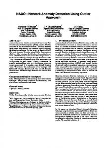
FIGURE 3. Six cases
IND(B) that contains element x. Rough sets are used in classification system, where we do not have complete knowledge of the system [31]. In any classification task the aim is to form various classes where each class contains objects that are not noticeably different. These indiscernible or indistinguishable objects can be viewed as basic building blocks (concepts) used to build a knowledge base about the real world. This kind of uncertainty is referred to as rough uncertainty. Rough uncertainty is formulated in terms of rough sets. In fuzzy sets, the membership of an element in a set is not crisp. It can be anything in between yes and no. The concept of fuzzy sets is important in pattern classification. Thus, fuzzy and rough sets represent different facets of uncertainty. Fuzziness deals with vagueness among overlapping sets [32]. On the other hand, rough sets deal with coarse non-overlapping concepts [33]. Neither roughness nor fuzziness depends on the occurrence of an event. In fuzzy sets, each granule of knowledge can have only one membership value for a particular class. However, rough sets assert that each granule may have different membership values for the same class. Thus, roughness appears due to indiscernibility in the input pattern set, and fuzziness is generated due to the vagueness present in the output class and the clusters. To model this type of situation, where both vagueness and approximation are present, the concept of fuzzy-rough sets [33] can be employed. 2.4.
Comparison proaches
of
outlier
Detection
Ap-
Outlier detection has largely focused on data that is univariate, and data with a known (or parametric or density-based) distribution. These two limitations have restricted the ability to apply outlier detection methods to large real-world databases which typically have many different fields and have no easy way of characterizing the multivariate distribution. The Computer Journal,
Approaches Case 1 Case 2 Case 3 Case 4 Case 5
Case 6
Distancebased Densitybased Soft computing
No
Yes
Yes
Yes
Yes
Yes
Yes
Yes
No
Yes
Partially Partially
Yes
Yes
Yes
Yes
Partially No
To evaluate the effectiveness of outlier detection methods, we consider six cases over the synthetic data set given in F ig. 3. In these figures, Oi is an object and Ci is cluster of objects. A distinct outlier object, (case 1 in F ig. 3) is one that cannot be included in any clusters, whereas a distinct inlier object (case 2) is inside of a cluster. An equidistant outlier (case 3) is the object which is at equal distance from the clusters, whereas non-distinct inlier (case 4) is that object located near the border of a cluster. The chaining effect (case 5) represents the objects which are situated in a straight line among the clusters. However, the staying together (case 6) effect represents the objects which are outliers on a straight line. A comparison table of three approaches in the context of these six cases over synthetic data is given in Table 1.
3.
NETWORK ANOMALY DETECTION
Unusual activities are outliers that are inconsistent with the remainder of data set [34]. An outlier is an observation that lies at an abnormal distance from other values in the dataset. In order to apply outlier detection to anomaly detection in the context of network intrusion detection, it is assumed by most researchers [10] that (1) the majority of the network connections are normal traffic. Only a small fraction of the traffic is malicious. (2) The attack traffic is statistically different from normal traffic. An anomaly detection technique identifies attacks based on deviations from the established profiles of normal activities. Activities that exceed thresholds of the deviations are identified as attacks. Thus, supervised and unsupervised outlier detection methods can find anomaly in network intrusion detection. Network intrusion detection systems [35] deal with detecting intrusions in network data. The primary reason for these intrusions is attacks launched by outside hackers who want to gain unauthorized access to the network to steal information or to disrupt the network. A typical setting is a large network of computers which is connected to the rest of the world through the Internet. Generally, detection of an intrusion in a network system is carried out based on two basic approaches - signature based and anomaly based. A signature based approach attempts to find attacks based on the previously stored patterns Vol. ??,
No. ??,
????
7 or signatures for known intrusions. However, an anomaly based approach can detect intrusions based on deviations from the previously stored profiles of normal activities, but also, capable of detecting unknown intrusions (or suspicious pattern). The NIDS does this by reading all incoming packets and trying to find suspicious patterns. 3.1.
Network Anomalies and Types
Anomaly detection attempts to find data patterns that are deviations in that they do not conform to expected behavior. These deviations or non-conforming patterns are anomalies. Based on the nature, context, behavior or cardinality, anomalies are generally classified into following three categories [10]: 1.
2.
3.
Point Anomalies- This simplest type of anomaly is an instance of the data that has been found to be anomalous with respect to the rest of the data. In a majority of applications, this type of anomaly occurs and a good amount of research addresses this issue. Contextual Anomalies- This type of anomaly (also known as conditional anomaly [36]) is defined for a data instance in a specific context. Generally, the notion of a context is induced by the structure in the data set. Two sets of attributes determine if a data instance belongs to this type of anomaly: (i) Contextual attributes and (ii) Behavioural attributes. Contextual attributes determine the context (or neighbourhood) for that instance. For example, in stock exchange or gene expression time series datasets, time is a contextual attribute that helps to specify the position of the instance in the entire sequence. However, behavioural attributes are responsible for the non-contextual characteristics of an instance. For example, in a spatial data set describing the average number of people infected by a specific disease in a country, the amount of infection at a specific location can be defined as a behavioural attribute. Collective Anomalies- These are collections of related data instances found to be anomalous with respect to the entire set of data. In collective anomaly, the individual data instances may not be anomalous by themselves, however, their collective occurrence is anomalous.
To handle the above types of anomalies, various detection techniques have been proposed over the decades. Especially, to handle the point anomaly type, distance-based approaches have been found suitable. However, the effectiveness of such techniques largely depends on the type of data, proximity measure or anomaly score used and the dimensionality of the data. In the case of contextual anomaly detection, both distance-based and density-based approaches have been found suitable. However, like the previous case, in the The Computer Journal,
case of distance-based outlier approaches, the proximity measure used, type of data, data dimensionality and the threshold measure play a vital role. The density-based approach can handle this type of anomaly effectively for uniformly distributed datasets. However, in the case of skewed distributions, an appropriate density threshold is required for handling the variable density situation. Collective anomaly is mostly handled by using densitybased approaches. However, in the identification of this type of anomalous patterns, other factors also play crucial role (such as compactness, and single linkage effects) 3.2.
Characterizing ANIDS
An ANIDS is an anomaly based network intrusion detection system. A variety of ANIDSs have been proposed since the mid 1980s. It is necessary to have a clear definition of anomaly in the context of network intrusion detection. The majority of current research on ANIDS does not explicitly state what constitute anomaly in their study [37]. In a recent survey [19], anomaly detection methods were classified into two classes: generative and discriminative. Generally, an ANIDS is characterized based on the following attributes: (i) nature and type of the input data, (ii) appropriateness of similarity/dissimilarity measures, (iii) labelling of data and (iv) reporting of anomalies. Next, we discuss each of these issues. 3.2.1. Types of Data A key aspect of any anomaly detection technique is the nature of the input data. The input is generally a collection of data instances or objects. Each data instance can be described using a set of attributes (also referred to as variables, characteristics, features, fields or dimensions). The attributes can be of different types such as binary, categorical or continuous. Each data instance may consist of only one attribute (univariate) or multiple attributes (multivariate). In the case of multivariate data instances, all attributes may be of the same type or may be a mixture of different data types. 3.2.2. Proximity measures Distance or similarity measures are necessary to solve many pattern recognition problems such as classification, clustering, and retrieval problems. From scientific and mathematical points of view, distance is defined as a quantitative degree of how far apart two objects are. A synonym for distance is dissimilarity. Distance measures satisfying the metric properties are simply called metric while non-metric distance measures are occasionally called divergence. A synonym for similarity is proximity and similarity measures are often called similarity coefficients. The selection of a proximity measure is very difficult because it depends upon the (i) the types of attributes in the data (ii) the dimensionality of data and (iii) the problem of weighing Vol. ??,
No. ??,
????
8
P.Gogoi D.K.Bhattacharyya B.Borah J.K.Kalita
data attributes. In the case of numeric data objects, their inherent geometric properties can be exploited naturally to define distance functions between two data points. Numeric objects may be discrete or continuous. A detailed discussion on the various proximity measures for numeric data can be found in [38]. Categorical attribute values cannot be naturally arranged as numerical values. Computing similarity between categorical data instances is not straightforward. Several data-driven similarity measures have been proposed [39] for categorical data. The behavior of such measures directly depends on the data. Mixed type datasets include categorical and numeric values. A common practice for clustering mixed datasets is to transform categorical values into numeric values and then use a proximity measure for numeric data. Another approach [27] is to compare the categorical values directly, in which two distinct values result in distance 1 while two identical values result in distance 0. 3.2.3. Data Labels The labels associated with a data instance denote if that instance is normal or anomalous. It should be noted that obtaining labelled data that is accurate as well as representative of all types of behaviours, is often prohibitively expensive. Labelling is often done manually by a human expert and hence requires substantial effort to obtain the labelled training data set. Several active learning approaches for creating labelled datasets have also been proposed [40]. Typically, getting a labelled set of anomalous data instances which cover all possible type of anomalous behavior is more difficult than getting labels for normal behavior. Moreover, anomalous behavior is often dynamic in nature, e.g., new types of anomalies may arise, for which there is no labelled training data. The KDD CUP ’99 dataset [41] is an evaluated intrusion data set with labelled training and testing data. Based on the extent to which labels are available, anomaly detection techniques can operate either in supervised or unsupervised approaches. A supervised approach usually trains the system with normal patterns and attempts to detect an attack based on its nonconformity with reference to normal patterns. In case of the KDD CUP ’99 dataset, the attack data are labelled into four classes – DoS (denial of service), R2L (remote to local), U2R (user to root), and probe. This defines the intrusion detection problem as a 5-class problem. If attack data are labelled into n possible classes, we have an (n + 1)-class problem at hand. An unsupervised approach does not need a labelled dataset. Once the system identifies the meaningful clusters, it applies the appropriate labelling techniques for identified clusters. A supervised approach has high detection rate (DR) and low false positive rate (FPR) of attack detection compared to an unsupervised The Computer Journal,
approach. Supervised approaches can detect known attacks whereas unsupervised approaches can detect unknown attacks as well. 3.2.4. Anomaly Scores Detection of anomalies depends on scoring techniques that assign an anomaly score to each instance in the test data depending on the degree to which that instance is considered an anomaly. Thus the output of such a technique is a ranked list of anomalies. An analyst may choose to either analyse the top few anomalies or use a cut-off threshold to select anomalies. Several anomaly score estimation techniques have been developed in the past decades. Some of them have been represented under the category of distance-based, density-based and machine learning or soft computing based approach. A Distance-based anomaly scores In this section, we introduce some of the popular distance-based anomaly score estimation techniques. A.1 LOADED (Link-based Outlier and Anomaly Detection in Evolving Data Sets) Anomaly Score [42] - Assume our data set contains both continuous and categorical attributes. Two data points pi and pj are considered linked if they are considerably similar to each other. Moreover, associated with each link is a link strength that captures the degree of linkage, and is determined using a similarity metric defined on the two points. The data points pi and pj are linked in a categorical attribute space if they have at least one attribute-value pair in common. The associated link strength is equal to the number of attribute-value pairs shared in common between the two points. A score function that generates high scores for outliers assigns score to a point that is inversely proportional to the sum of the strengths of all its links. To estimate this score efficiently, ideas from frequent itemset mining are used. Let I be the set of all possible attribute-value pairs in the data set M . Let D = {d : d ∈ P owerSet(I) ∧ ∀i,j:i!=j di · attrib $= dj · attrib}
be the set of all itemsets, where an attribute only occurs once per itemset. The score function for a categorical attribute is defined as: , !+ 1 |sup(d) ≤ s (7) Score1 (pi ) = |d| d⊆pi
where pi is an ordered set of categorical attributes. sup(d) is the number of points pi in the data set where d ⊆ pi , otherwise known as support of itemset d. |d| is the number of attribute-value pairs in d. s is a user-defined threshold of minimum support or minimum number of links. A point is defined to be linked to another point in the mixed data space if they are linked together in Vol. ??,
No. ??,
????
9 the categorical data space and if their continuous attributes adhere to the joint distribution as indicated by the correlation matrix. Points that violate these conditions are defined to be outliers. The modified score function for mixed attribute data is as follows: , !+ 1 |(C1 ∨ C2 ) ∧ C3 is true Score2 (pi ) = |d| d⊆pi
(8)
where C1 : sup(d) ≤ s, C2 : at least δ% of the correlation coefficients disagree with the distribution followed by the continuous attributes for point pi , and C3 : C1 or C2 hold true for every superset of d in pi . Condition C1 is the same condition used to find outliers in a categorical data space using Score1 (pi ). Condition C2 adds continuous attribute checks to Score1 (pi ). Condition C3 is a heuristic and allows for more efficient processing because if an itemset does not satisfy conditions C1 and C2 , none of its subsets are considered. A.2 RELOADED (REduced memory LOADED) Anomaly Score [43]- An anomalous data point can be defined as one that has a subset of attributes that take on unusual values given the values of the other attributes. When all categorical attributes of a data point have been processed, the anomaly score of the data point is computed as a function of the count of incorrect predictions and the violation score as below: ( ! m i−W ) j j=1 i Vτ AnomalyScore[Pi ] = + (9) m mn2 where Wj is the cumulative number of incorrect predictions of categorical attribute j for the previous i data points. There are m categorical attributes and n continuous attributes. Vτ is cumulative violation score of point Pi . B Density-based anomaly scores Here, we introduce a few density-based anomaly score estimation techniques. B.1 ODMAD (Outlier Detection for Mixed Attribute Datasets) Anomaly Score [27] - This score can be used in an approach that mines outliers from data containing both categorical and continuous attributes. The ODMAD score is computed for each point taking into consideration the irregularity of the categorical values, the continuous values, and the relationship between the two spaces in the dataset. A good indicator to decide if point Xi is an outlier in the categorical attribute space is the score value, Score1 , defined below: The Computer Journal,
!
Score1 (Xi ) =
d⊆Xi ∧supp(d)