Output Feedback Control of the Nonlinear Aeroelastic ... - CiteSeerX

Journal of Guidance, Control and Dynamics vol. 25, no. 2, Mar.-Apr. 2002, pp. 302 – 308

Output Feedback Control of the Nonlinear Aeroelastic Response of a Slender Wing Mayuresh J. Patil∗ and Dewey H. Hodges† Georgia Institute of Technology, Atlanta, Georgia 30332-0150 This paper presents the design of optimal constant gain output feedback based controllers for a nonlinear aeroelastic system. Controllers are designed for flutter suppression as well as gust-load alleviation. This controller architecture is one of the simplest, using direct feedback of the sensor outputs, but its performance is highly dependent on sensor selection and placement. Also, optimal design of such controllers require an accurate knowledge of the expected disturbance mode and gust spectrum. This paper presents results pertaining to the performance of SOF controllers for aeroelastic control (linear and nonlinear) and compares it to that of LQR and LQG controllers. Controllers are designed for various sensor placement. The gain and phase margins of the various controllers are also presented to understand the robustness characteristics. For optimal sensor placement and with knowledge of the disturbance, the constant gain output feedback controller performance and robustness was found to be equivalent to that of linear quadratic regulator and linear quadratic Gaussian controllers for the example considered. These controllers were also shown to be very easy to alter and combine with other controllers/filters for better overall system response.

Introduction

ear) and compares it to that of LQR and LQG controllers. The SOF controllers are designed for various sensor placement. The gain and phase margins of SOF controllers are also presented to understand the robustness characteristics.

Active aeroelastic control has been a topic of active research for the past two decades. Control design for flutter suppression and gust-load alleviation has been a focus of many previous researchers, for example, Mukhopadhyay1 and Crawley.2 Most of the control synthesis in previous investigations has been accomplished by linear optimal control theory, specifically Linear Quadratic Regulator (LQR) and Linear Quadratic Gaussian (LQG) control architecture. An LQR design is not practical because it requires the knowledge of the complete state-space. In most of the practical aeroelastic control problems it is impossible to sense all the states of the system. On the other hand, LQG controllers are dynamic controllers that have the same order as the assumed plant. Real-time implementation of high-order controllers is also quite problematic. There has not been much work focusing on the use of Optimal Static (Constant Gain) Output Feedback (SOF) controllers in aeroelastic applications. Waszak and Srinathkumar3 and Mukhopadhyay4 have designed classical controller based on constant gain output feedback coupled with polezero placement to achieve flutter suppression. In the present work, SOF controllers are based on linear quadratic optimization theory and lead to optimal performance with low controller complexity. SOF controllers feed back a linear combination of the sensor outputs and thus are very easy to implement. The use of SOF in aeroelastic flutter suppression and gust alleviation systems would lead to considerable simplification of the control law and ease in implementation. Due to the simplicity of SOF controllers they can be easily changed as well as combined with other control systems to get better overall characteristics. For example, excellent controller gain roll-off at high frequencies can be achieved by combining an SOF controller with a low-pass filter. SOF controllers can also be used with gain scheduling to generate efficient non-linear control. On the other hand, SOF controllers use direct feedback of the sensor outputs and thus sensor placement plays a very important role in such controllers. To achieve maximum performance the sensors need to be placed in the best possible location so as to sense the most important variables. Also unlike an LQR controller, SOF controllers are optimal only for the assumed disturbance (to the system) and thus are not robust to disturbance uncertainty. This paper presents results pertaining to the performance of SOF controllers in aeroelastic control (linear and nonlin-

Nonlinear Aeroelastic Model The aeroelastic model developed in Ref. 5 is used in the present work. The aeroelastic model is used to generate a nominal model based on the linearized aeroelastic system equations, which is used for control synthesis. In its complete nonlinear form, the model is used to simulate the open-loop as well as closed-loop nonlinear aeroelastic response of the wing. The structural formulation used in the present research is based on the mixed variational formulation for dynamics of moving beams.6 Equations of motion are generated by including the appropriate energies in the variational statement followed by application of calculus of variations. The finite-state aerodynamic theory of Peters and co-workers7 is a natural choice for low-order, high-fidelity state-space representation of the aerodynamics. It accounts for large airfoil motion as well as small deformation of the airfoil, e.g., trailing edge flap deflection. The complete aeroelastic formulation is described in detail by Patil8 and is presented here briefly for the sake of completeness. The structural equations of motion of the wing can be expressed in terms of nonlinear structural operator (FS ) and nonlinear aerodynamic operator (FL ) as ˙ − FL (X, Y, X) ˙ =0 FS (X, X)

(1)

where the vector X denotes the set of structural variables, and the vector Y denotes the set of aerodynamic induced flow variables. Similarly, we can separate the aerodynamic induced flow equations that model the unsteady wake effects in terms of an induced flow operator (FI ) and a downwash operator (FW ) as ˙ + FI (Y, Y˙ ) = 0 −FW (X)

(2)

Specialized Solutions

Equations (1) and (2) represent a set of coupled nonlinear differential equations modeling the dynamics of the coupled aeroelastic system. The solutions of interest can be expressed in the form       ¯ ˆ X X X(t) = + (3) ¯ Y Y Yˆ (t)

∗ Post-Doctoral Fellow, School of Aerospace Engineering. Member, AIAA. Presently, Research Assistant Professor, Duke University. † Professor, School of Aerospace Engineering. Fellow, AIAA.

Presented as AIAA Paper No. 2000-1627 at the AIAA/ASME/AHS Adaptive Structures Forum, Atlanta, Georgia, April 3 – 6, 2000. Copyright c 2001 by Mayuresh J. Patil and Dewey H. Hodges. Published by the
American Institute of Aeronautics and Astronautics, Inc. with permission.

where (¯) represents a nonlinear steady-state (equilibrium) solution and (ˆ) represents a linearized perturbation about 302

303

PATIL AND HODGES

the nonlinear equilibrium. Such a decomposition of the solution leads to two possibilities: nonlinear (large deformation) static equilibrium and linearized (small perturbation) dynamics at the equilibrium. Nonlinear equilibrium solution For the steady-state (equilibrium) solution one gets Y¯ identically equal to zero (from Eq. 2). Thus, one has to solve a set of algebraic nonlinear equations given by ¯ 0) − FL (X, ¯ 0, 0) = 0 FS (X,

(4)

The Jacobian matrix of the above set of nonlinear equations can be obtained analytically and is found to be very sparse.9 The steady-state solution can thus be found very efficiently using Newton-Raphson method. Linear small perturbation solution By perturbing Eqs. (1) and (2) about the calculated nonlinear steady state (using Eq. 3), the linearized set of equations can be written as     ∂FS ∂FL ˆ˙ − 0 X ˙ ˙ ∂X ∂X ∂FI W ˙ ¯ − ∂F X=X Yˆ ˙ ∂X ∂ Y˙ Y =0  ∂F     (5) S L L ˆ − ∂F − ∂F 0 X ∂X ∂X ∂Y + = ∂FI ¯ X=X 0 0 Yˆ ∂Y Y =0

These equations describe the small amplitude (linear) dynamics of the system around the calculated (nonlinear) steady state. Now assuming the dynamic modes to be of the form est , the above equations can be solved as an eigenvalue problem to get the damping, frequency and mode shape of the various modes. The stability condition of the aeroelastic system at various operating trim conditions can thus be obtained by perturbing the nonlinear equations of motion about the various nonlinear equilibrium solutions. The above set of linear dynamic equations is used as a nominal system to design linear optimal controller. Nonlinear dynamic solution To investigate the nonlinear dynamics of the aeroelastic system a time history has to be obtained using the complete nonlinear equations of motion. Space-time finite elements are used in the present work for time marching.8 Using space-time finite elements on the complete nonlinear system equations (1) and (2), one gets the time marching algorithm as a set of nonlinear algebraic equations FSt (Xi , Xf ) − FLt (Xi , Xf , Yi , Yf ) = 0 t −FW (Xi , Xf ) + FIt (Yi , Yf ) = 0

(6)

where subscripts i, f , represent the variable values at the t initial and final time, and FSt , FLt , FW , FIt are the nonlinear structural, aerodynamics, wake and inflow operators calculated using space-time finite elements.10 If the initial conditions and time interval are specified, the variable values at the final condition are obtained by solving the set of nonlinear algebraic equations. These nonlinear time-marching equations are used for open- and closed-loop simulation of the system. System Order Reduction

Before a controller is designed for the aeroelastic system, the linearized equations of motion (Eq. 5) of the system needs to be converted to a low-order, state-space form. The original total number of variables of the complete nonlinear system (and the linearized form) is around 30×n, where n is the number of finite elements used to model the wing. The break up of the 30 variables for each element is, 3 each for displacement (u), rotation (θ), internal force (F ), internal moment (M ), linear momentum (P ), angular momentum (H), and 6 each for induced flow states (λ) and stall states. For an eight element model of the wing this total is 240,

which is quite large. Some of the equations, e.g., the straindisplacement relations, have no time derivatives, and thus these equations can be used to represent the force and moment in terms of the displacements and rotations, reducing the order of the system to 24 × n. Also, in the nominal conditions considered here, there are no stall states leading to 18 × n variables. The final reduction in the number of variables and equations (and thus order of the nominal system) comes from the fact that the extensional and shear rigidities are very high and thus the corresponding strains are negligibly low. Thus a zero shear and zero extension approximation could be used to write the displacements and linear momentum variables in terms of the rotations and angular momentum variables. This further reduces the number of structural equations in half. The final count of variables is 12 × n, which includes three rotational variables and their time derivatives and six induced flow states per element. The displacement variables can always be recovered from the rotation variables.

Static Output Feedback Controller SOF controllers are based on direct feedback of the sensor output. Unlike an LQR controller, an SOF design does not assume the availability of all the system states for feedback. Rather, it is assumed that only a few linear combinations of system states are available (directly from the sensors). An optimal SOF controller aims to find the feedback gains that optimize a given performance index. Theory supporting the problem of optimal SOF for linear, multi-variable systems was first presented by Levine and Athans.11 A solution technique for solving the nonlinear matrix equations was also presented. A recent paper by Syrmos et al.12 gives the survey of the various SOF techniques, including optimal SOF. The theory pertaining to optimal SOF is presented here briefly. Given an nth -order Linear Time Invariant (LTI) stabilizable system x(t) ˙ = Ax(t) + Bu(t) + Dw(t) y(t) = Cx(t)

(7)

where x ∈ n are the system states, A is the system dynamics matrix in state-space form, u ∈ m are the actuator commands, B is the control actuation matrix, y ∈ p are the sensor measurement, C is the matrix relating the sensor measurements to the state variables, w is zero mean unit intensity white noise process, and D is the matrix of noise intensity. Assuming constant gain output feedback of the form u(t) = Ky(t)

(8)

one can determine feedback gains K such that it stabilizes the closed-loop system and minimize the quadratic performance measure given by  t  1 xT (τ )Qx(τ ) + uT (τ )Ru(τ ) dτ J(K) = lim E t→∞ t 0 (9) where Q ≥ 0 and R > 0 are state and control weighting matrices. The solution to the optimization problem given above is K = −R−1 B T SP C T (CP C)−1

(10)

where P and S are given by a set of coupled nonlinear matrix equations in terms of system parameters and K. Thus, the calculation of K involves the solution of three equations including the above equation for K and the Lyapunov equations given below 0 = ATc S + SAc + Q − C T K T RKC 0 = Ac P + P ATc + V

(11)

304

PATIL AND HODGES

where Ac = A + BKC, and V = DDT . The solution of the above set of coupled nonlinear equations can be calculated using a variety of iterative algorithms. Only a few of these algorithms have been proved to be convergent to a local minimum. Many other algorithms, though not proven to be convergent, do converge in most of the practical cases. The computational effort required also varies. A detailed survey of the various computational methods used to solve the optimal SOF problem is presented by Makila and Toivonen.13 Two algorithms have been used in results presented here: the (Broyden, Fletcher, Goldfarb, and Shanno) BFGS14 and an algorithm proposed by Moerder and Calise.15

0.5m

1m

16m

Results The example considered for the results presented in the present work is a high-aspect-ratio wing similar to those likely to be used in High-Altitude, Long-Endurance (HALE) aircraft. HALE aircraft are becoming increasingly common in various civil as well as military roles, including, reconnaissance, remote sensing, data relay station etc. But with the increase in the span of the wing (required for higher lift-todrag ratio) the wing is likely to encounter various detrimental aeroelastic response and stability problems. The aim of the present example is to present a simple study to illustrate the effective use of SOF for improving the aeroelastic characteristics of slender wings. HALE Wing Model

10m

5m

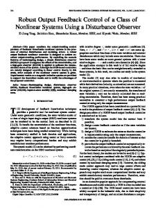
The example HALE wing considered is a slender wing of half-span aspect ratio of 16 (chord of 1 m). Fig. 1 shows an illustration of the HALE aircraft under consideration. The stiffness and inertial characteristics of the wing are detailed in Table 1. The nominal flight condition is a speed of 25 m/s at an altitude of 20 km. The flutter speed of the undeformed wing has been determined to be 32.21 m/s at the same altitude (see Ref. 16). The control design goals include, (i) extending the flutter envelop (closed-loop flutter speed) to at least 35 m/s by active control, and (ii) gustload alleviation at the nominal speed of 25 m/s. Sensor and Actuator

Various sensor placement strategies are considered. The aeroelastic system is dominated by the torsion and bending deformations. Thus twist sensors (for torsion) and curvature sensors (for bending) and the corresponding twist-rate and curvature-rate sensors are used. The SOF controllers are denoted by the sensors used. 1α denotes root-twist and roottwist-rate sensors, 2α denotes twist and twist-rate sensors at the root as well as mid-span, 3α denotes twist and twistrate sensors at the root, one-third spanwise position and two-third spanwise position. Such addition of sensors leads to progressively more information on higher modes. The curvature sensors are denoted similarly with 1h denoting the curvature and curvature-rate sensors at the root. Control is achieved by a flap at the wing tip. One of the aims of this paper is to show the effect of sensor placement on the effectiveness of SOF control. Flutter Suppression

The first study involves flutter suppression for the HALE wing at 35 m/s. The system matrices A, B, C are obtained by transforming the Jacobian matrix as described in the earlier sections. The controller is optimized for minimum control. Thus, the state is not penalized (Q = 0) and the control weight matrix is assumed unity (R = 1). A unit amplitude uncorrelated process noise is assumed to affect all the structural equations of motion equally. Results obtained from an SOF controller are compared to those from an LQR controller. As discussed earlier, an LQR controller cannot be practically implemented, because some the states of the system are unknown. Thus, an LQR controller must be accompanied by a state estimator, such as a Kalman filter.

Fig. 1

Illustration of the aircraft under consideration

tip vertical displacement (m)

PATIL AND HODGES 0.3 controlled uncontrolled

0.2 0.1 0 −0.1 0

0.5

1

1.5

2

2.5 time (s)

3

3.5

4

4.5

5

30

tip twist (deg)

20 10 0 −10 −20 0

0.5

1

1.5

2

2.5 time (s)

3

3.5

4

4.5

5

0.5

1

1.5

2

2.5 time (s)

3

3.5

4

4.5

5

control deflection (deg)

1 0.5 0 −0.5 −1 0

Fig. 2 SOF applied for flutter suppression at flight speed of 35 m/s

Once an estimator is added the resulting dynamic controller increases the controller complexity considerably. Though impractical, an LQR controller gives the best achievable performance and is thus a good baseline to gauge the optimality of an SOF controller. Linear SOF Controller Table 2 shows the results for control cost and closed loop damping due to various SOF controllers. As seen in Table 2, the SOF controller using just two-sensor feedback can give very good performance. For example, if one uses just roottwist and root-twist-rate feedback, the system is stabilized with 7% more cost, which in turn means 3.5% increase in control root mean square (rms) value. Also the closed-loop damping of the flutter mode is quite close to that provided by an LQR controller. Thus, with the data from just two sensors the SOF controller is able to control flutter with a control cost close to that of an LQR controller, which for the present example requires 96 states for feedback. As the number of twist sensors is increased, the performance and the stability improves slightly. On the other hand, feeding back only root-curvature and root-curvature-rate sensors cannot stabilize the system. This is because the aeroelastic energy transfer is dominated by the torsional instability that in turn transfers some energy to the bending mode. Thus, the knowledge of torsional variables is very important for a stabilizing controller design. To test the controller effectiveness, the HALE wing model is simulated with and without the controller. Fig. 2 shows the controlled and uncontrolled time history of the wing at 35 m/s with an initial bending deflection of 0.1 m at the tip. The controller with root-twist and root-twist-rate feedback is used in the simulation presented. The flutter is effectively suppressed by SOF control. SOF gives a good stabilizing controller with a proper choice of sensors. The performance comparisons with an LQR controller are also quite favorable. However, it should be pointed out that SOF gives the optimal performance for

305

the given disturbance (the same level of disturbance was assumed to be affecting all structural equations), whereas an LQR controller gives the best performance for any disturbance (since the LQR solution is independent of D, the matrix of noise intensity). Thus, if the disturbance were such that the aerodynamic equations were more affected, or that the structural equations were affected in a different mode, then one would not get good performance for the new disturbance using the original SOF controller. However, the performance of the LQR is still the best achievable, and consequently for a random disturbance the performance of an SOF controller would not be as close to that of an LQR controller. To design an optimal SOF controller, the aeroelastician would thus have to be able to accurately predict the amount of atmospheric disturbance, which would affect the aeroelastic system. Nonlinear SOF Controller Due to the simplicity of the SOF controller, it can be easily combined with gain scheduling to obtain a nonlinear controller. To demonstrate the ease of designing a nonlinear controller with SOF, a simple nonlinear controller is designed to control the nonlinear phenomena of limit cycle oscillations (LCO). It should be noted here that it is the insight into the nonlinear physical mechanisms responsible for the LCO that leads to a design of a simple nonlinear controller. Before the design of the nonlinear controller is explained, it is helpful to discuss the nonlinear limit cycle oscillation results presented in Patil et al.10 It has been shown therein that a wing curved due to lift forces exhibits behavior that is completely different from that of an undeformed wing. In fact, curved wings lead to instability at speeds much lower then the linear flutter speed. The dominant nonlinearity stems from wing bending, as is exhibited in wing tip displacement. The wing model when linearized about trim conditions at various levels of wing tip displacement, leads to various linearized systems. The linearized system eigenvalues exhibit drastic changes in the stability of the wing versus bending. For example, the HALE wing at 30 m/s is stable if linear analysis is used. There is a decrease in stability margin with curving of beam and at a tip displacement of around 0.6 m it becomes unstable. The tip displacement is thus a good parameter on which to base a nonlinear controller. Details on the type of nonlinearity in the wing is given in Ref. 10. A nonlinear controller is designed using dynamic gain scheduling, based on the tip displacement. A series of SOF controllers are designed at intervals of tip displacement. Again, root-strain and root-strain-rate are fed back, and the controller is linearly interpolated at in-between tip displacements. Fig. 3 shows the effect of such a nonlinear controller on the aeroelastic behavior of the HALE wing at 30 m/s when disturbed by a tip displacement of 2 m. The uncontrolled case gets attracted to a limit cycle oscillation, but the controlled wing approaches the undeformed stable equilibrium. If the damping of various modes is evaluated, one finds that even without control the first bending mode is damped, so that the bending deformation settles to an equilibrium value. As the wing oscillates about this bent configuration, a torsional mode is excited causing the wing to gain energy from the flow and transfer it back to the bending modes. The nonlinear SOF controller does not let the torsional energy increase, thus effectively suppressing the torsional mode and avoiding LCOs. The use of SOF truly simplifies the gain-scheduling mechanism, since only two control parameters, i.e., the feedback gains corresponding to root twist and root-twist rate, define the controller. Thus, to practically implement such a gain-scheduled controller the control computer would have to store a very small number of parameters. If one compares this SOF controller with gain-scheduled, observer-based, controllers, the simplicity of SOF controllers is obvious.

tip vertical displacement (m)

306

PATIL AND HODGES

for the low-pass filter plus SOF combination as compared to that of an LQG controller, with better roll-off characteristics, and a simple implementation.

2.5 2

controlled uncontrolled

1.5 1 0.5 0 0

5

10

15

10

15

10

15

time (s)

tip twist (deg)

40 20 0 −20 −40 0

5 time (s)

control deflection (deg)

1 0 −1 −2 −3 −4 −5 0

5 time (s)

Fig. 3 Nonlinear SOF controller applied to LCO control at 30 m/s

Combining SOF with a Low-Pass Filter Before ending this section on flutter suppression the SOF controller is compared to an LQG controller, i.e., an LQR controller in series with a Kalman estimator. LQG is an optimal dynamic output feedback controller that gives optimal performance for the case in which only few states of the system are sensed. On the other hand, the controller is very complex as compared to simple constant output feedback. Since the SOF controllers are designed under the assumption of zero sensor noise, the LQG controllers are also designed by using negligibly small sensor noise (the sensor noise matrix is reduced till the cost converges to a value). Table 3 shows the performance predictions for an LQG controller as compared to SOF controllers. As seen in the table, the LQG controller performance is not as good as that of an LQR controller but is only slightly better than that of an SOF controller. Thus, it is seen that LQG cannot be preferred over SOF for the small increase in performance as LQG is accompanied by a drastic increase in complexity. There are some characteristics of LQG controllers that make them a better choice as compared to SOF controllers. One of these is the high-frequency roll-off, meaning that the high-frequency unmodeled dynamics of the system are not affected by the controller (controller spill-over). Thus, the risk of destabilizing the system at high frequencies is reduced. One can introduce high-frequency roll-off in SOF by using a low-pass filter (LPF) in series with the SOF controller. Such characteristics have been shown earlier for second order acceleration feedback controllers.17 In this example a fixed, second-order, low-pass filter of frequency cutoff 100 rad/s and damping factor of 1.0 is used. As can be expected, such a low-pass filter will change the phase characteristics of the combined controller, thus leading to a decrease in the controller performance. But, the SOF controller could be reoptimized by assuming it to be attached to a low-pass filter. The reoptimized combination of the low-pass filter and SOF leads to a simple yet very effective controller. The control rms is only 1.33% higher

Gain and Phase Margins Finally, one of the most desired properties of a controller is robustness. Robustness leads to reliable controller performance in the face of plant or controller uncertainty. Stability margins are a good indication of the controller robustness to gain and phase shifts. Table 4 shows the stability margin predictions for the various controllers under investigation. As expected, the low-authority LQR controller has a gain margin of −6.02 db and +∞ db and phase margin of ±60◦ . The LQG controller has similar lower gain margin and phase margins. There is a degradation in the upper gain margin to around +12 db (but still ensuring stability at controller gains up to four times the nominal). As to the SOF controller, it shows gain and phase margins similar to the LQG design. Thus, SOF controller can be expected to have equivalent robustness properties. By adding a LPF to the SOF controller there is a shift in the phase margin. The phase shift is introduced because the LPF itself has a phase shift of around 25◦ at the unstable frequency. This phase shift is overcome by reoptimizing the SOF controller. Such a reoptimized controller regains the characteristics of the stand-alone SOF. Thus, a reoptimized SOF+LPF controller has performance, high-frequency roll-off, and stability margins very close to those of an LQG controller, but without the associated complexity. To summarize, with proper choice of sensors, an SOF controller can be designed that has performance close to that of an LQR controller. It is possible to modify the simple SOF controller for control of nonlinear system response. High-frequency roll-off can be achieved by combining such a controller with a low-pass filter. Finally, the SOF controllers also have gain and phase margins equivalent to LQR/LQG controllers. The SOF controllers can thus be quite effective for flutter suppression. Gust-Load Alleviation

Aircraft are exposed to various levels of wind and gust levels depending on its flight. Such external disturbances lead to a structural response of varying magnitude. Gust-load alleviation problem aims to keep the disturbance response of the wing low. Low disturbance response helps in extending the fatigue life of the structure as well as to improve ride quality. Gust Model For the results presented here the gust model is based on the continuous atmospheric turbulence model given by Bisplinghoff et al.18 Using this model, the power spectrum of atmospheric turbulence in terms of space frequency can be represented as Φ

ω   (ft/s)2 U

rad/ft

=

0.060 0.000004 +

 ω 2

(12)

U

¯ ), one could write the power freFor a given speed (U quency spectrum of atmospheric turbulence in SI units as  Φ (ω)

(m/s)

2

rad/s

=

¯ 0.078U 2 ¯ 0.000043U + ω 2

(13)

The above equation at a given flight speed has the form of the power spectrum of a first order dynamic system excited by white noise. Thus, the atmospheric turbulence model can be easily represented in terms of a single state dynamic system. This equation is added to the aeroelastic system equations. The output of the gust equation to white noise is the source of disturbance to the aeroelastic system.

307

PATIL AND HODGES

Conclusion

SOF Design for Gust Alleviation The HALE wing is considered at nominal flight speed of 25 m/s. The state cost component of the performance index is defined in terms of the structural energy19 as Js = xTs [K]xs + x˙ Ts [M ]x˙ s , where xs are the structural states. Table 5 shows the state and control cost associated with SOF controllers using various sensors. The results are very different from those obtained for flutter suppression. For flutter suppression, twist sensing was most important since the unstable mode was dominant in twist. For gust alleviation, curvature (bending) sensing leads to the best performance. Here, the low frequency bending modes are excited the most by the gust. Curvature sensing is thus most important for gust-load alleviation since it senses the modes that are most disturbed. Comparison with LQR Designs The way to represent an LQR controller for a system with a gust state is unclear; because, even though the gust state is part of the mathematical system which is used for design, it is not a part of the actual system. Thus, whether or not to include the gust state feedback is unclear. There are three LQR-like controllers designs possible. The first one is denoted as LQR (white noise) and is based on the assumption of a white noise disturbance to the system, i.e., the gust state equation is not included in LQR design. The second, LQR (including gust model), is the LQR design based on the model that includes the gust state. Thus, the controller uses the gust state feedback for control. The third controller denoted by LQR (FSF) is a full state feedback that assumes the existence of gust state for control design, but the feedback is dependent only on the original aeroelastic system states. All controllers are implemented on the complete aeroelastic system including the gust model. Table 6 gives the performance results for various LQR designs and compares it with SOF design. If LQR controller is designed without considering the actual gust spectrum, i.e., assuming a white noise, then the design is not useful in controlling the response of the assumed gust. This is because, though LQR is by design an optimal controller for any disturbance spatial mode (any distribution of disturbance to the various equations), it assumes that the disturbance is a white noise process affecting all the frequencies (and thus modes) equally. However, the actual gust spectrum is such that it affects a few lower modes much more than any of the higher modes. Consequently even if the higher frequency modes have a lower stability margin these modes are not as affected due to the lower excitation power and thus need not be given control priority over the lower modes. Thus, the results obtained using an LQR (white noise) controller are not good. Now, if the gust model is included and an LQR controller is designed assuming gust state feedback, it gives the best achievable results. But this model is inconsistent in that knowledge of the gust state is assumed, which by definition is quite random. Though unachievable, it is a good baseline result for comparison. On the other hand, if a full original model state feedback is designed, the performance gives the best achievable results of constant gain output feedback. It is seen that this result is quite close to that obtained by using only root-curvature and root-curvature-rate feedback. Thus, using just a pair of sensors, i.e., for root curvature and root-curvature rate, an SOF controller could be designed to give performance within 1% of the performance one would achieve by feeding back all the 96 states. This again points out that effective SOF controllers could be designed by choosing the right sensors. In summary, SOF controllers can be effective in gust alleviation with proper choice of sensor. LQR performance using white noise disturbance assumptions do not lead to effective controllers. Inclusion of a proper gust model is necessary for optimal performance.

Static output feedback (SOF) controllers were designed for flutter suppression and gust-load alleviation of a slender wing. SOF controller performance was a strong function of the choice of sensors and the sensor placement. For flutter suppression, root twist and root-twist rate were the most important variables, and thus sensing these variables led to an SOF controller with performance equivalent to that of an LQR controller. On the other hand, sensing root curvature was of importance for gust-load alleviation due to the dominant effect of gust on the bending modes. A nonlinear SOF controller was designed by gain scheduling over various wing displacements (a dominant nonlinearity). The nonlinear SOF controller was implemented along with the complete wing nonlinear aeroelastic simulation and was shown to control limit cycle oscillations generated by large disturbances. A low-pass filter was designed and coupled with the static output feedback to get good roll-off characteristics, leading to robustness with respect to highfrequency dynamics. Also, the gain and phase margins of the SOF controller were calculated and where shown to be close to those of the LQG controller. Gust-load alleviation characteristics for an SOF controller were again quite close to that of full state feedback controller. It was further shown that, though the LQR design is optimal for all disturbances (in terms of the equation affected), it is highly dependent on the gust spectrum (as is SOF). Thus, an LQR design based on a white noise gust spectrum led to sub-optimal results. The knowledge of gust state is very important for efficient control, so that an LQR controller which is designed assuming knowledge of gust state gives the best results. But, an LQR design based on feedback of just the system states (a full-state feedback without the gust state) gives performance close to that obtained by SOF with just two sensors.

Acknowledgments The authors would like to acknowledge Prof. W. Haddad and Dr. J. Corrado from Georgia Tech for their help in the optimal static output feedback design. They also provided some parts of the basic SOF synthesis code. The authors would also like to acknowledge helpful discussions with Prof. A. Calise of Georgia Tech. This work was supported by the U.S. Air Force Office of Scientific Research (Grant number F49620-98-1-0032), the technical monitor of which was Maj. Brian P. Sanders.

References 1

Mukhopadhyay, V., “Flutter Suppression Control Law Design and Testing for the Active Flexible Wing,” Journal of Aircraft, Vol. 32, No. 1, Jan.-Feb. 1995, pp. 45 – 51. 2 Lin, C. Y., Crawley, E. F., and Heeg, J., “Open- and ClosedLoop Results of a Strain-Actuated Active Aeroelastic Wing,” Journal of Aircraft, Vol. 33, No. 5, Sep. – Oct. 1996, pp. 987 – 994. 3 Waszak, M. R. and Srinathkumar, S., “Flutter Suppression for the Active Flexible Wing: A Classical Design,” Journal of Aircraft, Vol. 32, No. 1, Jan. – Feb. 1995, pp. 61 – 67. 4 Mukhopadhyay, V., “Transonic Flutter Suppression Control Law Design and Wind-Tunnel Test Results,” Journal of Guidance, Control, and Dynamics, Vol. 23, No. 5, Sep. – Oct. 2000, pp. 930 – 937. 5 Patil, M. J., Hodges, D. H., and Cesnik, C. E. S., “Nonlinear Aeroelastic Analysis of Complete Aircraft in Subsonic Flow,” Journal of Aircraft, Vol. 37, No. 5, Sep – Oct 2000, pp. 753 – 760. 6 Hodges, D. H., “A Mixed Variational Formulation Based on Exact Intrinsic Equations for Dynamics of Moving Beams,” International Journal of Solids and Structures, Vol. 26, No. 11, 1990, pp. 1253 – 1273. 7 Peters, D. A. and Johnson, M. J., “Finite-State Airloads for Deformable Airfoils on Fixed and Rotating Wings,” Symposium on Aeroelasticity and Fluid/Structure Interaction, Proceedings of the Winter Annual Meeting, ASME, Chicago, November 6 – 11 1994, pp. 1 – 28, AD-Vol. 44. 8 Patil, M. J., Nonlinear Aeroelastic Analysis, Flight Dynamics, and Control of a Complete Aircraft, Ph.D. thesis, Georgia Institute of Technology, Atlanta, Georgia, May 1999. 9 Hodges, D. H., Shang, X., and Cesnik, C. E. S., “Finite Element Solution of Nonlinear Intrinsic Equations for Curved Composite

308

PATIL AND HODGES

Table 1

Model data

WING Half span 16 m Chord 1 m Mass per unit length 0.75 kg/m Mom. Inertia (50% chord) 0.1 kg m Spanwise elastic axis 50% chord Center of gravity 50% chord Bending rigidity 2 × 104 N m2 Torsional rigidity 1 × 104 N m2 Bending rigidity (edgewise) 5 × 106 N m2 FLIGHT CONDITION Altitude 20 km Density of air 0.0889 kg/m3 Beams,” Journal of the American Helicopter Society, Vol. 41, No. 4, Oct. 1996, pp. 313 – 321. 10 Patil, M. J., Hodges, D. H., and Cesnik, C. E. S., “Limit Cycle Oscillations in High-Aspect-Ratio Wings,” Journal of Fluids and Structures, Vol. 15, No. 1, Jan. 2001, pp. 107 – 132. 11 Levine, W. S. and Athans, M., “On the Determination of the Optimal Constant Output Feedback Gains for Linear Multivariable Systems,” IEEE Transactions on Automatic Control, Vol. AC-15, No. 1, Feb. 1970, pp. 44 – 48. 12 Syrmos, V. L., Abdallah, C. T., Dorato, P., and Grigoriadis, K., “Static Output Feedback – A Survey,” Automatica, Vol. 33, No. 2, 1997, pp. 125 – 137. 13 Makila, P. M. and Toivonen, H. T., “Computational Methods for Parametric LQ Problems – A Survey,” IEEE Transactions on Automatic Control, Vol. AC-32, No. 8, August 1987, pp. 658 – 671. 14 Shanno, D. F. and Phua, K. H., “Numerical Comparison of Several Variable-Metric Algorithms,” Journal of Optimization Theoryand Applications, Vol. 25, 1978, pp. 507 – 518. 15 Moerder, D. D. and Calise, A. J., “Convergence of a Numerical Algorithm for Calculating Optimal Output Feedback Gains,” IEEE Transactions on Automatic Control, Vol. AC-30, No. 9, September 1985, pp. 900 – 903. 16 Patil, M. J., Hodges, D. H., and Cesnik, C. E. S., “Nonlinear Aeroelasticity and Flight Dynamics of High-Altitude Long-Endurance Aircraft,” Journal of Aircraft, Vol. 38, No. 1, Jan. – Feb. 2001, pp. 88 – 94. 17 Bayon De Noyer, M. and Hanagud, S., “A Comparison of H2 Optimized Design and Cross-Over Point Design for Acceleration Feedback Control,” Proceedings of the 39th Structures, Structural Dynamics, and Materials Conference, Long Beach, California, April 20 – 23, 1998, pp. 3250 – 3258. 18 Bisplinghoff, R. L., Ashley, H., and Halfman, R. L., Aeroelasticity, Addison-Wesley Publishing Co., Reading, Massachusetts, 1955. 19 Belvin, W. K. and Park, K. C., “Structural Tailoring and Feedback Control Synthesis: An Interdisciplinary Approach,” Journal of Guidance, Control, and Dynamics, Vol. 13, No. 3, May – Jun. 1990, pp. 424 – 429.

309

PATIL AND HODGES

Table 2

Sensors config. System LQR SOF 1α SOF 2α SOF 3α SOF 1h SOF 1α1h

SOF performance for various sensor configurations

Control cost 0 586.90 628.56 626.29 625.13 Unstable 622.33

% increment in cont. rms w.r.t. LQR – 0% 3.49% 3.30% 3.21% – 2.97%

Table 3

Sensors config. System LQR LQG 1α SOF 1α SOF 1α + LPF Reoptimized

Control cost 0 586.90 607.46 626.29 796.13 623.72

Table 4

c.l.eig.val. real part 1.0323 -1.0323 -1.0323 -0.9190 -0.6438 -0.9396

c.l.eig.val. imag part 21.1978 21.1978 21.1978 21.2219 22.0321 21.2038

Comparison of the stability margins

gain margins −6.02 db +∞ db −5.84 db +12.03 db −5.44 db +9.66 db −4.30 db +9.50 db −5.69 db +9.81 db

phase margins −60◦ +60◦ −58.70◦ +56.15◦ −58.98◦ +54.87◦ −80.29◦ +28.36◦ −59.28◦ +56.29◦

SOF performance for gust alleviation at 25 m/s

Sensors config. SOF 1α SOF 1h SOF 2h SOF 3h SOF 1α1h

Table 6

c.l.eig.val. imag part 21.1978 21.1978 21.2219 21.2646 21.2528 – 21.2242

SOF/LPF performance

% increment in cont rms w.r.t. LQR w.r.t. LQG – – 0% – 1.74% 0% 3.49% 1.72% 16.47% 14.48% 3.09% 1.33%

Sensors config LQR LQG 1α SOF 1α SOF 1α + LPF SOF 1α + LPF (reopt.)

Table 5

c.l.eig.val. real part 1.0323 -1.0323 -0.9190 -0.9118 -0.9167 – -0.9598

Performance measure 74.614 62.788 62.598 62.580 62.605

State cost 74.215 53.342 53.016 52.985 53.033

Control cost 0.399 9.446 9.582 9.595 9.572

Comparison of SOF performance with LQR

Sensors config. SOF 1h LQR (white noise) LQR (gust model) LQR (FSF)

Performance measure 62.788 75.015 48.584 62.552

State cost 53.342 75.014 38.968 52.938

Control cost 9.446 0.00025 9.616 9.614