function of time can be described by the bathtub curve. The fail- ure rate is the conditional probability per unit time that a failure occurs at a specific (possibly ...
When are Multiple Gate Errors Significant in Logic Circuits? Smita Krishnaswamy, Igor L. Markov, John P. Hayes {smita,imarkov,jhayes}@eecs.umich.edu Advanced Computer Architecture Lab, University of Michigan, Ann Arbor
Abstract Most recent works on soft errors only address circuit reliability under single gate errors caused by SEUs. In this paper, we compare the probabilities of single and multiple errors. We formulate a criterion based on gate error probabilities for considering multiple gate errors in circuit reliability. Gate error probabilities are increased by technology trends such as the down-scaling of device features and process variation. The probability of multiple errors is generally higher when there is correlation between gate errors. We discuss several examples of correlated errors such as systematic errors and SEUs with a common radiation source. The correlation decreases the number of error combinations to be considered, thereby making multiple gate errors easier to simulate and analyze. We conclude by briefly discussing methods to model multiple errors. 1
Motivation
Trends in chip technology include the down-scaling of device features and increasing process variation in VLSI and molecular circuits. These trends increase the likelihood of circuits experiencing soft errors. A soft error is a signal in a logic circuit which has an incorrect logic value but does not imply a permanent defect. Soft errors are often transient in nature. A gate error is an incorrect signal at the output of a gate. In previous research, it is commonly assumed that there is only one such error in the entire circuit for each clock cycle. Thus, the focus of soft error research has been on the effects of single-event upsets (SEUs)— an SEU occurs when a charged particle deposits some of its charge on a microelectronic device. Tools such as SERA [10], and FASER [11] attempt to predict the probability with which a single gate error (caused by an SEU), propagates to a primary output of the CMOS circuit in question. In contrast to those works, our error representation is not technology-specific since we seek to study general trends in several domains including nano- and quantum circuits. In this paper, we compare the probability of single gate errors (SGEs) to simultaneous multiple gate errors (MGEs). An MGE is a collection of SGEs which occur in the same clock cycle. The SGEs that constitute an MGE may mutually mask each other depending upon the input vector. In general, the output error probability that results from an MGE cannot be easily predicted from resultant output error probabilities of the constituent SGEs (see Example 1). Many circuits have more fan-in than fanout. For instance, the average gate-to-output ratio in the ISCAS85 benchmark suite is ≈ 35. Therefore, MGEs have to be specifically modeled in these determine output error probabilities. However, mutual masking may not occur often in circuits with a high degree of fanout and relatively little fan-in. In these types of circuits the separate modeling of the constituent SGEs may be enough to predict output error probabilities.
Figure 1: Sample circuit. Example 1 Suppose the circuit in Figure 1 has an MGE consisting of gate errors at AND and X1, namely bit-flips with probability 0.10, regardless of the input value. Table 1 lists the output error probabilities for each primary input combination. Note that output error probabilities under the MGE are not equal to the sum of the output error probabilities for the two SGEs. Output error probabilities depend on how the errors logically mask each other for each input combination. Input 00 01 10 11
Output Error Prob. Combined X1 AND 0.10 0 0.10 0.18 0.10 0.10 0 0 0 0.18 0.10 0.10
Table 1: Output error probabilities for circuit in Figure 1.
Classical circuits are generally only tested for single errors due to the assumption that the mean time between failures (MTBF) exceeds the time it takes to repair a single error. Circuits may be repaired or discarded before multiple errors are allowed to accumulate. This assumption does not hold for soft errors. Typically, soft errors are a result of inherently unreliable components or external radiation effects and cannot be repaired. The remaining portion of this paper is organized as follows: Section 2 discusses the probability of MGEs with each gate having an independent probability of error, the effect of technology trends on gate error probabilities is discussed in Section 3, Section 4 discusses examples of situations where there is a correlation between gate errors due to a common error source, Section 5 discusses techniques for handling MGEs and Section 6 concludes the paper.
2
When Error Rates are High
0.01
In this section, we derive a criterion for the probability of gate error per clock cycle for a significant number of MGEs. For the purposes of projection, we assume an average probability of gate error Perr (g). The probability of gate error averaged over typical operating conditions (altitude, temperature, neutron flux, etc) and over all the types of gates in a circuit. If gates experience error independently, the probability of experiencing k errors in a circuit with n gates is given by the binomial random variable: � � n Pk = Perr (g)k (1 − Perr (g))n−k (1) k
1e-04
Pcrit
1e-06
1e-10
1e-12
1e-14 100
PSGE = P1 = nPerr (g)(1 − Perr (g))n−1
n
PMGE =
∑
k=2
n k
B(p, k + 1, n + k) B(1, k + 1, n + k)
1e+12
1e+14
PSM (g) ∝ exp(
(4)
(5)
A closed-form solution for this equation is difficult to find. However, as Figure 2 shows us the minimum Perr (g) needed to meet the criteria in Equation 4, Pcrit , decreases with the number of gates according to the following Equation when C = 100: Pcrit ≈ 0.23 × 10−N
(8)
1 Qcmax (g) )× Qs (g) τclk
(9)
PSM (g) is dependent upon the threshold voltage, if the threshold voltage is low, it is likely that a noisy-0 signal can be interpreted as a 1. PSM (g) is proportional to the clock frequency because at high clock frequencies the phenomenon of ground bounce,i.e., the raising or lowering of the voltage on a ground pin, can cause signals to be misinterpreted in comparison to ground. Trends in VLSI circuits which can affect Perr (g) include:
To find the gate error probability at which MGE’s become important we can solve for Perr (g) in the equation: 1 − F(Perr (g), n, 2) > F(Perr (g)n, 1) − F (Perr (g), n, 0)
Qcmax (g) ) Qs (g)
F is the neutron flux given in particles per unit area per unit time, A is the gate area, and τclk is the clock period. Qcmax (g) is the critical charge required to overcome the threshold voltage and Qs (g) is the charge collection efficiency of the gate in question. PSM (g) is the probability that a signal which is logically 0 is interpreted as a 1 or vice versa by gate g.
Perr (g)k (1−Perr (g))n−k = 1−F(n, 2, p) (3)
C × PMGE > PSGE
• Increasing gate density — results in reduction of gate area A which in turn decreases PSEU (g), but this effect is balanced by an increase in the number of gates. Furthermore, if gates are smaller, a single event may cause multiple upsets due to increased proximity among gates.
(6)
In a circuit with only 100 gates Pcrit = .025, in a circuit with 1, 000, 000 gates Pcrit = .025 × 10−6 . The criterion derived in this section is somewhat optimistic since in many cases correlation between errors make MGEs more common. For instance, as gates become smaller a single SEU can cause multiple errors. Such situations are discussed in more detail in Section 4.
• Decreasing threshold voltage — less energy is required to overcome the threshold voltage so PSM (g) and PSEU (g) are both increased [4]. • Increasing clock speed — decreases the PSEU (g) since τclk decreases but PSM (g) increases due to the ground-bounce phenomenon described above [3].
When Gates Reach Nanoscale
• Decreasing clock speed — this is a trend in low-power computing. Decreasing the clock speed will increase τclk in Equation 8 and therefore increase PSEU (g).
As device features continue to shrink, quantum effects may eventually dominate circuit behavior. Quantum-mechanical behaviors are inherently probabilistic, but certain probabilistic effects become apparent even at much larger scales. We classify mechanisms by which probabilistic gate errors occur into two main categories: external particle strikes (SEU) and signal misinterpretations (SM). The total probability of gate error can be expressed as: Perr (g) = Pg (SEU ∪ SM) (7) 1
1e+10
PSEU (g) ∝ F × A × τclk × exp(
MGE’s become of interest to hardware designers when PMGE comes close to PSGE , that is for some constant C > 0:
3
1e+08
PSEU (g) is the probability that gate g experiences an SEU and is dependent on the neutron flux F at the current altitude. The authors in [8] give an estimate for this probability as follows:
Rp where B(p, k + 1, n + k) = 0 uk (1 − u)n−k−1 δu 1
�
1e+06
Figure 2: The minimum probability of gate error, Pcrit , required to meet criteria in Equation 4 as the number of gates increases.
(2)
The probability of MGEs can be derived from the cumulative distribution function (cdf) F(n, k, p) for the binomial distribution. F(n, k, p) is calculated using the regularized incomplete betafunction
�
10000
Number of Gates
The probability of an SGE is:
F(n, k, p) = Ip (k + 1, n + k) =
1e-08
Emerging technologies which are vying to replace CMOS circuits include quantum circuits, quantum dots and molecular circuits. General nanotechnology trends include: • Process variations — causes differences in threshold voltage between gates which can increase PSM (g).
The beta-function can be written in terms of the gamma-function as B(a, b) = On natural numbers Γ(n) = n!
Γ(a)Γ(b) Γ(a+b) .
2
Example 3 Quantum circuits often experience systematic error due to similar resonant frequencies for all qubits in a quantum system. When one qubit is operated upon, all other qubits experience a rotational error. This situation can be described by a bimodal distribution with the modes at 0 and n − 1. A probability distribution of this type can be a sum of two normal distributions Px =
−(x − 1) −(x − (n − 1)) 1 (exp( ) + exp( )) 4π 2 2
(13)
PMGE can be calculated as in Example 2 as the average of the two normal distributions. Example 4 In the case of time-related failures of circuit components, the fault probabilities of different components are related by the hidden time variable. The failure rate of any component as a function of time can be described by the bathtub curve. The failure rate is the conditional probability per unit time that a failure occurs at a specific (possibly infinitesimally small) time interval. The bathtub curve is piece-wise defined and has three regions: the first region is the infant mortality region, the second region is a constant failure rate, the third region is the wear-out region which is characterized by an increasing failure rate.
Figure 3: Single event multiple upset. Source:NASA • No gain in molecular circuits — since the gates in these circuits do not have a power supply source, signals tend to become attenuated. Gates that are towards the end of logic blocks tend to mistakenly interpret signals as the low logic value, thereby increasing PSM (g). 4
k0 − k 1 t + λ Perr (g|t) = { λ c2 (t − t0 ) + λ
i f 0 < t ≤ k0 /k1 i f k0 /k1 < t ≤ t0 i f t0 ≤ t
(14)
PMGE is calculated by a method similar to that of Equation 3 with Perr (g) replaced by Perr (g|t).
When Errors Have Common Sources 5
Often, SGEs arise from a single source thereby making the probability of an MGE higher. An obvious instance of this is a single event multiple upset, where a single neutron hits multiple neighboring gates. Figure 3 from NASA JPL’s Space Radiation Effects group [9] shows how a single event multiple upset occurs. Note that several damage clusters are produced by the movement of silicon atoms after an initial SEU collision. Unlike the independent SGE’s which constitute MGEs in Section 2, the incidence of such highly-correlated errors is proportional to SGE rates and somewhat less sensitive to clock speed. A more subtle example is systematic errors in quantum circuits. A systematic error is when an operation on a particular gate erroneously affects all other gates in the circuit. In environments where there is a radiation source, the fact that one gate experiences an SEU indicates that other gates may experience SEUs as well. In these situations the correlations between gate errors make PMGE higher while also making MGEs somewhat easier to handle. In this section we discuss several examples of correlated errors.
The total output error in a circuit consisting of unreliable gates can be derived by the union of the probabilities of gate errors. For a circuit with n gates, this probability is found using the principle of inclusion and exclusion: � � n n Perr (circuit) = ∑ (−1)i+1 Perr (g)i (15) k i=1
However, if Perr (g) < Pcrit , then the total output error probability in the circuit can be estimated as the sum of all single gate error probabilities. Perr (circuit) = n × Perr (g)
−(x − µ) 1 exp( ) 2π 2
Any particular combination of x errors has probability � � n Px / x 1 PMGE = 1 − F(2) = 1 − √ 2π
Z 2 0
exp(
−(x − 2) )dx 2
(16)
The absolute error in this estimate is: � � n Perr (g)2 2
Example 2 Suppose that a high-altitude environment has a neutron flux rate of F particles per unit area per second. For a circuit with N gates and area A, this makes all combinations of F × N × A errors more likely than other error combinations. The total number of errors can be described by a normal distribution with a mean of µ = F × N × A errors. Px =
Calculating MGE Probabilities
In practice, the error is smaller since many gate errors become attenuated before they latch as output errors. In addition, even in some cases where Perr (g) > Pcrit , there are some types of circuits where mutual error masking does not occur often. In these circuits, the probability of an MGE is calculated by the sum of probabilities of constituent SGE. The probability of two errors mutually masking each other can be upper bounded by the number of pairs of convergent paths in a circuit. This is calculated by counting the number of gates in each of the output logic cones of the circuit. For a circuit with n gates, k outputs and logic cone sizes {l1 , l2 , . . . lk } the number of pairs of gate with potential convergence is:
(10)
(11)
Cpaths = (12)
3
�
n 2
�
k
−∑
i=1
�
li 2
�
(17)
We can upper bound the probability of mutual masking by: C � paths� n 2
error correlations of the type discussed above can be encoded as Bayesian networks once the parent nodes are identified and the local implications are determined. Probabilistic reasoning can then be used to determine the impact of these correlated errors on the outputs.
(18)
Circuits which have relatively little fan-in have a lower probability of mutual masking. A decoder is an example of such a circuit.
6
Conclusion
In this paper we determined conditions under which simultaneous multiple gate errors (MGEs) become significant. We discussed how trends in nanotechnology will affect the likelihood of these errors. We analyze MGE probabilities under independent and correlated gate error assumptions with various examples of correlated gate errors. Correlations between gate errors can often make them easier to simulate and analyze. Future work seeks to develop a probabilistic model which captures gate error correlations.
Example 5 A decoder with 3-inputs and 8-outputs (as shown in Figure 4) has logic cones of sizes {4, 3, 3, 3, 2, 2, 2, 1}. For this circuit, Cpaths = 18 and the total number of path-pairs is 55, therefore the probability of mutual masking can be bounded by 18/55. For a 4-input decoder this bound decreases to 65/190.
References [1] D. Alexandrescu, L. Anghel and M. Nicolaidis, “New Methods for Evaluating the Impact of Single Event Transients in VDSM ICs,” Proc. DFT 2002, pp. 99-107. [2] R.I. Bahar, J. Mundy and J. Chan, “A Probabilistic Based Design Methodology for Nanoscale Computation,” Proc. ICCAD 2003, pp. 480-486. [3] E. Dupont, M. Nicolaidis, P. Rohr, “Embedded Robustness IPs for Transient-Error-Free ICs,” IEEE Design & Test, May/June 2002, pp. 56-70. [4] D. Ernst et al.,“Razor: A Low-Power Pipeline Based on Circuit-Level Timing Speculation,” Proc. MICRO 2003, pp. 7-19. [5] S. Krishnaswamy, I. L. Markov and J. P. Hayes, “Testing Logic Circuits for Transient Faults,” Proc. ETS 2005, pp. 102-107. [6] S. Krishnaswamy et al., “Accurate Reliability Evaluation and Enhancement via Probabilistic Transfer Matrices,” Proc. DATE 2005, pp. 282-287. [7] K. Mohanram and N. A. Touba, “Cost-Effective Approach for Reducing Soft Error Failure Rate in Logic Circuits,” Proc. ITC 2003, pp. 893-901. [8] P. Shivakumar et. al, “Modeling the Effect of Technology Trends on Soft Error Rate of Combinational Logic,” Proc. DSN 2002, pp. 389-398. [9] Radiation Effects Group, NASA JPL “Space Radiation Effects On Microelectronics,” http://parts.jpl.nasa.gov/resources.htm. [10] M. Zhang and N. R. Shanbhag, “A Soft Error Rate Analysis (SERA) Methodology,” Proc. ICCAD 2004, pp. 111-118. [11] B. Zhang, W. Wang and M. Orshansky,“FASER: Fast Analysis of Soft Error Susceptibility for Cell-based Designs”, to appear in ISQED 2006.
Figure 4: 3-input decoder. In general, output error probabilities may be predicted by random or partial simulation methods which handle single errors as long as the number of multiple errors to consider is reasonably small. There may be prohibitively many combinations of SGEs that could form an MGE, however, correlation between SGEs can lessen the number of combinations that need to be considered. For instance, in Example 2, we can simply consider all combinations of F SGEs since the probability of fewer or more errors is small. This reduces the number of combinations from 2n to nF . In Example 4, we can test for all possible combinations of µ errors where µ is the average probability of error for the binomial distribution with each component having independent error rate Perr (g|t). Alternatively, probabilistic reasoning methods can be used to encode dependencies between errors and gates. In order to capture all of the dependencies between gate errors it is necessary to have the complete joint fault probability table. For instance, in order to calculate PSGE it is necessary to calculate the joint probability error of the following form: PSGE = Perr (g1 , g2 , . . . gn ) + Perr (g1 , g2 , . . . gn ) . . .
(19)
Here gi indicates that gate gi has no error. We can often identify causal links among SGEs and hidden variables such that the joint probability can be expressed as a chain of conditional probabilities. Example 6 Suppose the hazard function of a device was as in Example 4. In this case Perr (g1 , g2 , . . . gn ) can be calculated by P(t)Perr (g1 |t)(1 − Perr (g2 |g1 ,t)) . . .
(20)
However, since g1 and g2 are conditionally independent, Equation 20 can be calculated by: P(t)Perr (g1 |t)(1 − Perr (g2 |t)) . . .
(21)
In [5] gate error probabilities are encoded in probabilistic transfer matrices (PTM). An MGE is modeled by a collection of PTMs with a non-zero probability of error. These probabilities are combined by gate connectivity to determine the effect of MGEs on the output. This work treats gate errors as independent. However, 4