Apr 24, 2006 - mW must be in the range (â2, 0) for Dov(0) to describe a single Dirac fermion in the continuum. The properties of Dov(0) have been studied in ...
Overlap Dirac operator at nonzero chemical potential and random matrix theory Jacques Bloch and Tilo Wettig Institute for Theoretical Physics, University of Regensburg, 93040 Regensburg, Germany (Dated: April 24, 2006) We show how to introduce a quark chemical potential in the overlap Dirac operator. The resulting operator satisfies a Ginsparg-Wilson relation and has exact zero modes. It is no longer γ5 -hermitian, but its nonreal eigenvalues still occur in pairs. We compute the spectral density of the operator on the lattice and show that, for small eigenvalues, the data agree with analytical predictions of nonhermitian chiral random matrix theory for both trivial and nontrivial topology.
arXiv:hep-lat/0604020v1 24 Apr 2006
PACS numbers: 12.38.Gc, 02.10.Yn
Recent years have seen great advances in two areas that at first sight seem to be totally unrelated: (i) the study of nonhermitian operators in the natural sciences [1] and (ii) the problem of chiral symmetry on the lattice [2]. In this article we focus on a problem in which both of these areas are relevant, namely quantum chromodynamics (QCD) at nonzero baryon (or quark) density, which is important for the study of relativistic heavy-ion collisions, neutron stars, and the early universe [3]. If a quark chemical potential µ is added to the QCD Dirac operator, the operator loses its hermiticity properties and its spectrum moves into the complex plane. This causes a variety of problems, both analytically and numerically. Lattice simulations are the main source of nonperturbative information about QCD, but at µ 6= 0 they cannot be performed by standard importance sampling methods because the measure of the Feynman path integral, which includes the complex fermion determinant, is no longer positive definite. While a generic solution to this so-called sign problem is unlikely to be found [4], a number of recent works have been able to make progress by circumventing the problem in various ways [5, 6, 7]. These methods all agree on the transition temperature from the hadronic to the quark-gluon phase in the regime µ/T . 1 [3]. A better analytical understanding of QCD at very high baryon density has been obtained by a number of methods [8], and the QCD phase diagram has been studied in model calculations based on symmetries [9]. Chiral random matrix theory (RMT) [10], which makes exact analytical predictions for the correlations of the small Dirac eigenvalues, has been extended to µ 6= 0 [11], and a mechanism was identified [12] by which the chiral condensate at µ 6= 0 is built up from the spectral density of the Dirac operator in an extended region of the complex plane, in stark contrast to the Banks-Casher mechanism at µ = 0. A first comparison of lattice data with RMT predictions at µ 6= 0 was made in Ref. [13] using staggered fermions. One issue with staggered fermions is that the topology of the gauge field is only visible in the Dirac spectrum if the lattice spacing is small and various improvement and/or smearing schemes are applied [14]. To
avoid these issues, we would like to work with a Dirac operator that implements a lattice version of chiral symmetry and has exact zero modes at finite lattice spacing. The overlap operator [15] satisfies these requirements at µ = 0. In the following, we show how the overlap operator can be modified to include a nonzero quark chemical potential [16, 17]. We then study the spectral properties of this operator as a function of µ and compare data from lattice simulations with RMT predictions. As we shall see, the overlap operator has exact zero modes also at nonzero µ, which allows us, for the first time, to test predictions of nonhermitian RMT for nontrivial topology. We begin with the well-known definition of the Wilson Dirac operator DW including a chemical potential µ [18], DW (µ) = 1 − κ
3 X i=1
� � Ti+ + Ti− − κ eµ T4+ + e−µ T4− ,
(Tν± )yx = (1 ± γν )U±ν (x)δy,x±ˆν ,
(1)
where κ = 1/(2mW + 8) with the Wilson mass mW , the U ∈ SU(3) are the lattice gauge fields, and the γν are the usual euclidean Dirac matrices. Unless displayed explicitly, the lattice spacing a is set to unity. The overlap operator is defined at µ = 0 by [15] Dov (0) = 1 + γ5 ε(γ5 DW (0)) ,
(2)
where ε is the matrix sign function and γ5 = γ1 γ2 γ3 γ4 . mW must be in the range (−2, 0) for Dov (0) to describe a single Dirac fermion in the continuum. The properties of Dov (0) have been studied in great detail in the past years. In particular, its eigenvalues are on a circle in the complex plane with center at (1, 0) and radius 1, its nonreal eigenvalues come in complex conjugate pairs, and it can have exact zero modes without fine-tuning. Dov (0) satisfies a Ginsparg-Wilson relation [19] of the form {D, γ5 } = Dγ5 D .
(3)
We now extend the definition of the overlap operator to µ 6= 0. The operator DW (0) in Eq. (2) is γ5 -hermitian, † i.e., γ5 DW (0)γ5 = DW (0), and therefore the operator γ5 DW (0) in the matrix sign function is hermitian. How-
2 ever, for µ 6= 0, DW (µ) is no longer γ5 -hermitian. Defining the overlap operator at nonzero µ by Dov (µ) = 1 + γ5 ε(γ5 DW (µ)) ,
(4)
we now need the sign function of a nonhermitian matrix. In general, a function f of a nonhermitian matrix A can be defined by a contour integral. A more convenient expression can be obtained if A is diagonalizable. In this case we can write A = U ΛU −1 , where U ∈ Gl(N, C) with N = dim(A) and Λ = diag(λ1 , . . . , λN ) with λi ∈ C. Then f (A) = U f (Λ)U −1 , where f (Λ) is a diagonal matrix with elements f (λi ). The sign function can be defined by [20] ε(A) = U sign(Re Λ)U −1 .
(5)
This definition ensures that ε2 (A) = 1 and gives the correct result if Λ is real. An equivalent definition is ε(A) = A(A2 )−1/2 [21]. Eqs. (4) and (5) constitute our definition of Dov (µ). The sign function is ill-defined if one of the λi lies on the imaginary axis. Also, it could happen that γ5 DW (µ) is not diagonalizable (one would then resort to a Jordan block decomposition). Both of these cases are only realized if one or more parameters are fine-tuned. This is unlikely to happen in realistic lattice simulations, and we therefore ignore these issues. It is relatively straightforward to derive the following properties of Dov (µ). • Dov (µ) is no longer γ5 -hermitian because for a nonhermitian matrix A we generically have ε† (A) 6= ε(A). † (−µ). Instead, Dov (µ) satisfies γ5 Dov (µ)γ5 = Dov • Dov (µ) still satisfies the Ginsparg-Wilson relation (3) because of ε2 (A) = 1. Thus, we still have a lattice version of chiral symmetry, and the operator has exact zero modes without fine-tuning. • The eigenvalues of Dov (µ) that are not equal to 0 or 2 no longer come in complex conjugate pairs, but every such eigenvalue λ (with eigenfunction ψ) is accompanied by a partner λ/(λ − 1) (with eigenfunction γ5 ψ). • At µ = 0, the mapping λ → z = 2λ/(2 − λ) projects the eigenvalues from the circle to the imaginary axis. At µ 6= 0, the same mapping projects the eigenvalues λ and λ/(λ − 1) to a pair ±z, which is the same pairing as for µ 6= 0 in the continuum. • The eigenfunctions of Dov (µ) corresponding to eigenvalue 0 or 2 can be arranged to have definite chirality. The numbers n± λ of modes with λ = 0, 2 and hγ5 i = ±1 − + − satisfy n+ 0 − n0 = −(n2 − n2 ). (Without fine-tuning, − + − we even have n0 = n2 = 0 or n+ 0 = n2 = 0, which is always the case in our lattice data below.) • Generically, Dov (µ) is not normal, i.e., DD† 6= D† D. We now turn to our (quenched) lattice simulations. The computation of the sign function of a nonhermitian matrix is very demanding. We are currently investigating various approximation schemes [22], but in this initial study we decided to compute the sign function and
1
1
µ=0.0 0.3
Im(λ)
Im(λ) 0.5
0.5
0
0
-0.5
-0.5
-1
-1 0
0.5
1
1.5 Re(λ)
0
2
0.2 0.4 Re(λ)
FIG. 1: Spectrum of Dov (µ) for µ = 0 and µ = 0.3 for a typical configuration. The figure on the right is a magnification of the region near zero.
to diagonalize Dov (µ) exactly using LAPACK. For the comparison with RMT we need high statistics, which restricts us to a very small lattice size. We have chosen the same parameter set as in Ref. [23] to be able to compare with previous results at µ = 0. The lattice size is V = 44 , the coupling in the standard Wilson action is β = 5.1, the Wilson mass is mW = −2, and the quark mass is mq = 0. The small lattice size forces us to use such a strong coupling to stay in the ergodic regime of QCD, see Eq. (11) below, but we expect the conclusions of this paper to remain valid at weaker couplings and correspondingly larger lattice sizes. The choice of mW = −2 is motivated by concerns about the locality of Dov (µ), although at V = 44 this question is largely academic. Our parameters are given in Table I. In Fig. 1 we show the spectrum of Dov (µ) for a typical configuration for µ = 0 and µ = 0.3. As expected, we see that the eigenvalues move away from the circle as µ is turned on. Another observation is that the number of zero modes of Dov (µ) for a given configuration can change as a function of µ, see Table I. This can be understood from the relation between the anomaly and the index of Dov [24, 25], − tr(γ5 Dov ) = 2 index(Dov ) ,
(6)
which we can show to remain valid at µ 6= 0. Using tr(γ5 Dov ) = tr[γ5 + ε(γ5 DW )] = tr[ε(γ5 DW )] and the fact that the eigenvalues of the sign function are +1 or W W −1, one has nW − − n+ = 2 index(Dov ), where n± denotes the number of eigenvalues of γ5 DW (µ) with real part ≷ 0. As µ changes, an eigenvalue of γ5 DW can move across the W imaginary axis. As a result, nW − − n+ changes by 2, and TABLE I: Number of configurations and distribution of the number ν of zero modes of Dov (µ) for various values of µ. µa
# config.
P (ν = 0)
P (ν = 1)
P (ν = 2)
0.0 0.1 0.2 0.3 1.0
6783 8703 5760 5760 2816
0.544 0.526 0.500 0.476 0.268
0.426 0.439 0.454 0.465 0.446
0.029 0.034 0.046 0.058 0.210
3 ρ(0,y) 0.4
0.15 ν=0
ν=0
0.3
ρ(0,y)
ρ(0,y) 0.08
ρ(0,y)
0.4
ν=0
0.06
ν=0
0.1 0.2
0.04 ν=1
0.05
0.1 0
ν=1
1
2
3
4 y
ρ(x,0) ν=0
0.06
0.06
0.04
0.04 ν=1
0.02
1
2
3
4 y
-1
0
ρ(x,yc) 0.3
1
x2
2
3
4 y
0
0.5
ν=0 0.2
ν=1
ν=1
ν=1 0
0 -2
1
0.4
0.02
-4
y=Im(ξ)
ρ(x,0)
ν=0
0
2
x4
ρ(x,yc) ν=0 yc=1.25
1
ν=0
0.04
0 -2
0 0
ρ(x,0)
0.02
0
ν=1
0 0
ρ(x,0) 0.08
0.08
ν=1
0.02
0 0
0.2
-6
-4
-2
0
2
4
ρ(x,yc)
0.2
-0.5
0
0.5 1 x=Re(ξ)
ρ(|ξ|) ν=0 yc=2.32
0.06
ν=0 yc=2.21
0.1
-1
x6
0.4 ν=0
0.04 0.2
0.05
0.1
ν=1 yc=2.91
ν=1 yc=2.61
0
0 -2
-1
0
1
x2
ν=1
ν=1 yc=2.74
0.02 0
-4
-2
0
2
x4
0 -6
-4
-2
0
2
4
x6
0
0.5
1 |ξ|
FIG. 2: Density of the small eigenvalues of Dov (µ) in the complex plane (after projecting λ → 2λ/(2 − λ) and rescaling by V Σ) for (from left to right) µ = 0.1, 0.2, 0.3, 1.0. The histograms are lattice data for ν = 0 and ν = 1, and the solid lines are the corresponding RMT prediction of Eq. (8), integrated over the bin size. Top: cut along the imaginary axis, middle: cut along the real axis, bottom: √ cut parallel to the real axis. The vertical lines indicate the fit interval. For µ = 1.0, the eigenvalues are rescaled by V Σ/2 α, the fit is a one-parameter fit to Eq. (10), and in the bottom plot the data are integrated over the phase.
thus index(Dov ) changes by 1, which explains the observation. We believe that this is a lattice artefact which will disappear in the continuum limit. (Also, the index theorem is violated at β = 5.1, but for the comparison with RMT only the number of zero modes matters.) ov PThe spectral density of Dov (µ) is given by ρ (λr , λi ) = h k δ(λ − λk )i with λ = λr + iλi , where the average is over configurations. The claim is that the distribution of the small eigenvalues of Dov (µ) is universal and given by RMT. The RMT model for the Dirac operator is [11] � � 0 iW + µ DRMT (µ) = , (7) iW † + µ 0 where W is a complex matrix of dimension n × (n + ν) with no further symmetries (we take ν ≥ 0 without loss of generality). The matrix in Eq. (7) has ν eigenvalues equal to zero. The spectral correlations of DRMT (µ) on the scale of the mean level spacing were computed in Refs. [26, 27, 28]. In the quenched approximation, the result for the microscopic spectral density reads � 2 � x + y2 x2 + y 2 y2 −x2 RMT 4α Kν e ρs (x, y) = 2πα 4α Z 1 2 × t dt e−2αt |Iν (tz)|2 , (8) 0
where z = x + iy, I and K are modified Bessel functions, and α = µ2 fπ2 V . To compare the lattice data to
this result, the eigenvalues λk need to be rescaled by a parameter 1/V Σ which is proportional to the mean level spacing near zero, � x y � 1 ov . (9) ρ , ρov (x, y) = s (V Σ)2 VΣ VΣ Σ and fπ are low-energy constants that can be obtained from a two-parameter fit of the lattice data, Eq. (9), to the RRMT prediction, Eq. (8). (The normalization is fixed by dx dy ρov (x, y) = 12V and does not introduce another parameter.) For x ≪ α, Eq. (8) simplifies to [29] ρRMT (x, y) → s
ξ |z|2 Kν (ξ) Iν (ξ) with ξ = . 2πα 4α
(10)
A fit of Eq. (9) to Eq. (10) then only involves the single parameter Σ/fπ . In Fig. 2 we compare our lattice data to the RMT prediction. We display various cuts of the eigenvalue density in the complex plane as explained in the figure captions. The data agree with the RMT predictions within our statistics. Σ and fπ were obtained by a combined fit to the ν = 0 and ν = 1 data for all three cuts and are displayed in Table II. (These numbers have no physical significance at β = 5.1.) Separate fits to the ν = 0 and ν = 1 data give results consistent with those in Table II. For µ = 1.0 we have fitted to Eq. (10) since the distribution of the small eigenvalues is radially symmetric up to
4 TABLE II: Fit results for Σ and fπ (see text). µa
Σa3
fπ a
Σa3 /fπ a
χ2 /dof
0.0 0.1 0.2 0.3 1.0
0.0816(6) 0.0812(11) 0.0785(14) 0.0824(17) –
– 0.261(6) 0.245(5) 0.248(5) –
– 0.311(5) 0.320(4) 0.332(4) 0.603(18)
1.10 0.67 0.78 1.03 0.42
|ξ| ∼ 0.7, and therefore Σ and fπ cannot be determined independently by a fit to Eq. (8). We note in passing that unfolding along the imaginary axis results in better agreement of the lattice data with RMT for larger values of y, but we shall not discuss this issue here since it is a finite-volume effect that will be unimportant on larger lattices. The RMT results are valid in the “ergodic regime” mπ , µ ≪
1 ≪Λ, L
(11)
where L4 = V , mπ is the Goldstone boson mass, and Λ is the mass scale of the lightest non-Goldstone particle. The rescaled eigenvalues z = λV √Σ should therefore be described by RMT for |z| ≪ fπ2 V (the √ dimensionless Thouless energy). For our data, fπ2 V ≈ 1 (this explains the choice of β = 5.1; for larger β this number would be even smaller). Nevertheless, the data seem to be described by RMT quite well even a bit beyond this expectation. Also, µ = 1.0 corresponds to µL = 4, which violates the inequality (11). The fact that RMT still works below the Thouless energy in this case means that the zero-momentum modes decouple from the partition function. A detailed study of the range of validity of RMT at µ 6= 0 as a function of the lattice parameters will be the subject of further work (see also Ref. [30]). In summary, we have shown how to include a quark chemical potential in the overlap operator. The operator still satisfies a Ginsparg-Wilson relation and has exact zero modes. The distribution of its small eigenvalues agrees with predictions of nonhermitian RMT for trivial and nontrivial topology. Our initial lattice study should be extended to weaker coupling, larger lattices, and better statistics. Work on approximative methods to enable such studies is in progress. For small volumes, reweighting with the fermion determinant should allow us to test RMT predictions for the unquenched theory [31]. This work was supported in part by DFG. We acknowledge illuminating discussions with W. Bietenholz, F. Knechtli, H. Neuberger, and J.J.M. Verbaarschot (whom we also thank for a critical reading of the manuscript). The simulations were performed on a QCDOC machine in Regensburg using USQCD software and Chroma [32]. We thank K. Goto for providing us with an optimized GotoBLAS for QCDOC.
[1] for a comprehensive list of applications and references, see M. Embree and L.N. Trefethen, Pseudospectra Gateway, http://www.comlab.ox.ac.uk/pseudospectra [2] for a review, see P. Hasenfratz, hep-lat/0406033 [3] for a review, see O. Philipsen, PoS LAT2005 (2005) 16 [4] M. Troyer and U.-J. Wiese, Phys. Rev. Lett. 94 (2005) 170201 [5] Z. Fodor and S.D. Katz, Phys. Lett. B 534 (2002) 87 [6] C.R. Allton et al., Phys. Rev. D 66 (2002) 074507 [7] P. de Forcrand and O. Philipsen, Nucl. Phys. B 642 (2002) 290; M. D’Elia and M.-P. Lombardo, Phys. Rev. D 67 (2003) 014505 [8] for a recent review, see M.G. Alford, Nucl. Phys. (Proc. Suppl.) 117 (2003) 65 and references therein [9] M.A. Halasz et al., Phys. Rev. D 58 (1998) 096007 [10] E.V. Shuryak and J.J.M. Verbaarschot, Nucl. Phys. A 560 (1993) 306; J.J.M. Verbaarschot, Phys. Rev. Lett. 72 (1994) 2531 [11] M.A. Stephanov, Phys. Rev. Lett. 76 (1996) 4472 [12] J.C. Osborn, K. Splittorff, and J.J.M. Verbaarschot, Phys. Rev. Lett. 94 (2005) 202001 [13] G. Akemann and T. Wettig, Phys. Rev. Lett. 92 (2004) 102002, Erratum ibid. 96 (2006) 029902 [14] F. Farchioni, I. Hip, and C.B. Lang, Phys. Lett. B 471 (1999) 58; E. Follana, A. Hart, and C.T.H. Davies, Phys. Rev. Lett. 93 (2004) 241601; S. D¨ urr, C. Hoelbling, and U. Wenger, Phys. Rev. D 70 (2004) 094502; K.Y. Wong and R.M. Woloshyn, Phys. Rev. D 71 (2005) 094508; E. Follana et al., Phys. Rev. D 72 (2005) 054501 [15] R. Narayanan and H. Neuberger, Nucl. Phys. B 443 (1995) 305; H. Neuberger, Phys. Lett. B 417 (1998) 141 [16] for a perfect lattice action at µ 6= 0, see W. Bietenholz and U.-J. Wiese, Phys. Lett. B 426 (1998) 114 [17] for an overlap-type operator at µ 6= 0 in momentum space, see W. Bietenholz and I. Hip, Nucl. Phys. B 570 (2000) 423 [18] P. Hasenfratz and F. Karsch, Phys. Lett. B 125 (1983) 308; J.B. Kogut et al., Nucl. Phys. B 225 (1983) 93 [19] P.H. Ginsparg and K.G. Wilson, Phys. Rev. D 25 (1982) 2649 [20] J.D. Roberts, Int. J. Control 32 (1980) 677 [21] N.J. Higham, Linear Algebra Appl. 212-213 (1994) 3 [22] J. Bloch, A. Frommer, B. Lang, and T. Wettig, in preparation [23] R.G. Edwards et al., Phys. Rev. Lett. 82 (1999) 4188 [24] R. Narayanan and H. Neuberger, Nucl. Phys. B 412 (1994) 574 [25] P. Hasenfratz, V. Laliena, and F. Niedermayer, Phys. Lett. B 427 (1998) 125; M. L¨ uscher, Phys. Lett. B 428 (1998) 342 [26] K. Splittorff and J.J.M. Verbaarschot, Nucl. Phys. B 683 (2004) 467 [27] J.C. Osborn, Phys. Rev. Lett. 93 (2004) 222001 [28] G. Akemann, J.C. Osborn, K. Splittorff, and J.J.M. Verbaarschot, Nucl. Phys. B 712 (2005) 287 [29] Eq. (479) in J.J.M. Verbaarschot, hep-th/0410211 [30] J.C. Osborn and T. Wettig, PoS LAT2005 (2005) 200 [31] G. Akemann and E. Bittner, hep-lat/0603004 [32] R.G. Edwards and B. Jo´ o, Nucl. Phys (Proc. Suppl.) 140 (2005) 832