Dirac operator and Ising model on a compact 2D random lattice

BI-TP 2001/22 LPT Orsay 01/89

arXiv:hep-lat/0110063v1 12 Oct 2001

Dirac operator and Ising model on a compact 2D random lattice L. Bogacz1,2 , Z. Burda1,2 , J. Jurkiewicz2 , A. Krzywicki3 , C. Petersen1 and B. Petersson1 1

Fakultät f¨ ur Physik, Universität Bielefeld P.O.Box 100131, D-33501 Bielefeld, Germany 2

3

Institute of Physics, Jagellonian University ul. Reymonta 4, 30-059 Krakow, Poland

Laboratoire de Physique Théorique, Bâtiment 210, Université Paris-Sud, 91405 Orsay, France Abstract

Lattice formulation of a fermionic field theory defined on a randomly triangulated compact manifold is discussed, with emphasis on the topological problem of defining spin structures on the manifold. An explicit construction is presented for the two-dimensional case and its relation with the Ising model is discussed. Furthermore, an exact realization of the KramersWannier duality for the two-dimensional Ising model on the manifold is considered. The global properties of the field are discussed. The importance of the GSO projection is stressed. This projection has to be performed for the duality to hold.

Introduction The massless Majorana free fermion theory belongs to the same universality class as the critical Ising model on a regular lattice [1, 2, 3, 4]. An explicit construction of the Majorana-Dirac-Wilson fermion field theory on a randomly triangulated plane was introduced in [5]. This theory was shown to be equivalent to the Ising model also outside the critical region. In ref.[5] Cartesian coordinates were assigned to the nodes of the lattice. The directions of the links and of the related gamma matrices were expressed in the global frame of the plane. This approach works for lattices embedded in a 1

flat background where one has at one’s disposal a global frame of the underlying geometry [6, 7, 8]. However, if one wants to generalize it to a lattice on a curved background where no global frame exists, a field of local frames [9, 10, 11] has to be introduced. This being done, one can put fermions on a curved manifold with any topology and one can eventually attack, for example, problems of field theory on a dynamical geometry like those encountered in string theory or in quantum gravity [14, 15, 16, 17, 18]. This generalization was partially carried out in [10, 11] where an explicit construction of the Majorana-Dirac-Wilson operators on curved compact two-dimensional lattices was introduced. Here we extend these studies. In particular, we discuss the significance of the GSO projection, which as in string theory also here plays an important physical role [12, 13]. We show that with a careful treatment of the global properties of the Dirac operator and of the spin structures on the manifold one can find a strict mathematical one-to-one equivalence between the partition function of the Majorana-Wilson fermions and that of the Ising model. We show explicitly that in our discretization of the Dirac operator on a compact manifold, the GSO projection - the summation over all spin structures - does remove the non-contractible fermionic loops, that is those not corresponding to the domain-walls of the corresponding Ising model. Further, we show that for the duality to hold exactly as a one-to-one map between the Ising model on a triangulation and on its dual lattice, a sort of GSO projection has also to be done. Different spin structures for the Ising field are simulated by physical cuts produced by the introduction of antiferromagnetic loops, which mimic antiperiodic fermionic boundary conditions. The paper is organized as follows. In section 1 we give an introduction to the problem of defining the Dirac operator on a compact manifold. It is text-book material [13, 20]. We recall it here for completeness, to keep the article self-contained. In section 2, we show how to adapt the standard Wilson discretization scheme of fermions on the regular translationally invariant hypercubic lattice [22] to the local-frame description, which can be generalized to the case of irregular curved lattices. In section 3, using as an example the standard toroidal regular lattice, we discuss the sign problem and the global properties of the fermionic field on a compact manifold. In section 4 we argue that in the case of irregular lattices the local frame description is particularly natural, and then in section 5 we show how to lift this construction to the spinorial representation. In doing this we introduce rotation matrices between neighboring frames which are crucial for the construction. In particular, using the spinorial representation of these matrices we are able to define in section 6 the Dirac-Wilson operator. The standard definition of the partition function representing quantum amplitudes is recalled in section 2

7. In this section we also list the properties of the mathematical expressions encountered in calculating the partition function. In section 8 we calculate the partition function using the hopping parameter expansion. The topological loop sign problem emerges naturally there. The issue of loop signs is discussed in more detail in section 9 where the sign is defined as a function of classes of loop homotopies. The relation between signs of non-contractible fermionic loops and of domain-walls in Ising model and the topological aspect of the duality is discussed in section 10. In section 11 we give two analytic examples, calculating the critical temperature of the Ising model on the honeycomb lattice and the critical value of the hopping parameter on the dynamical triangulation, making use of the existence of the exact map between the Ising model and the fermionic model. We close with a short discussion.

1

Preliminaries

The aim of this paper is to discretize a theory of fermions on a random, possibly fluctuating geometry. Let us first recall some basic facts about the continuum formulation of this problem. Consider a D-dimensional compact Riemannian manifold, on which a coordinate system ξ µ is defined. If a nonsingular change of coordinates ξ µ → ′ ξ µ is performed at some point x on the manifold, then a linear transformation of the components of any vector or tensor field in the tangent space at x has also to be carried out, in order to ensure the invariance of the theory under coordinate transformations. For vectors, the matrix of this linear transformation reads : ′ ∂ξ µ µ Aν (x) = (x) . (1) ∂ξ ν Since the change of coordinates is not singular, the determinant of A is nonzero. The matrices A thus form a linear group of non-singular real matrices GL(D, R). The basic difficulty in any attempt to apply the transformation law (1) to a fermionic field is that the group GL(D, R) has no spinorial representation. In other words, one cannot directly apply the information encoded in A to transform a spinor when changing the coordinates. In order to overcome this difficulty one has to restrict somehow the group GL(D, R) to its SO(D) subgroup, which does have spinorial half-integer representations. One can do this by introducing an additional field of local orthonormal frames. More precisely, at each point x of the manifold one introduces a basis ea (x), a = 1, . . . , D, in the tangent space, which obeys ea (x) · eb (x) = δab 3

(orthonormality) and e1 (x) ∧ e2 (x) . . . ∧ eD (x) > 0 (orientability), where the symbols · and ∧ denote the internal and external products. Expressed in a given coordinate system ξ µ , the orthonormality and orientability conditions read : gµν (x) eµa (x) eνb (x) = δab ,

e(x) ≡ det eµa (x) =

q

g(x) > 0 .

(2)

The matrix eµa (x) is called the vielbein. It is non-singular, and one can denote its inverse matrix by eaµ (x). Thus one has, for instance, eaµ (x)ebν (x)δab = gµν (x). With these vectors one can also associate gamma matrices γ a , {γ a , γ b } = 2δ ab , that can be chosen so as to have the same numerical values γ a for all points x. One can write the Dirac matrices in the curved coordinates as γ µ (x) = eµa (x)γ a . The price to pay for introducing this new field is that one also has to introduce an additional connection on top of the Levy-Civita connection. The new connection ω (which is called the spin connection) allows one to calculate covariant derivatives of objects that have frame indices. For instance, the covariant derivative of the vielbein itself is given by ∇µ eνa = ∂µ eνa + Γµνλ eλa − ωµa b eνb

(3)

The reward is that the spin connection can be lifted to the spinorial representation, and we can calculate the covariant derivatives of spinors as well : 1 ∇µ ψ = ∂µ ψ + ωµab σ ab ψ , 2

(4)

where σ ab = 2i1 [γ a , γ b ] is the rotation generator in the spinorial representation. The action for fermions coupled to gravity can now be written as : S=

1 2

=

1 2

R R

dD ξ e ψ¯ γ µ ∇µ ψ =

1 2

R

dD x ψ¯ (γ a · ∇a ) ψ

¯ D(x, y) ψ(y) . d x d y ψ(x) D

D

(5)

The Dirac operator on the manifold is D(x, y) = δ(x − y) γ a (x) · ∇a (x) ,

(6)

or, less formally, just γ · D. We shall discretize this operator in the next section. Before doing so, however, let us discuss its topological properties. Locally, one can always define a continuously varying field of frames. However, doing this globally for a compact manifold is usually impossible. 4

What can be done instead in this case is to cover the manifold with open patches, in each of which one can separately define a continuous field of frames, and for any region of overlapping patches U and V provide transition matrices for recalculating the frames when going from one patch to the other : [eU ]a (x) = [RU V ]ba [eV ]b (x) .

(7)

Here, the transition function RU V is a SO(D) rotation matrix. It follows that the spinors in the overlapping region can be recalculated as : [ψU ]α (x) = [RU V ]βα [ψV ]β (x) .

(8)

where RU V is an image of RU V in the spinorial representation. In a region where three patches U, V, W intersect, the transition matrices must obviously fulfill the following self-consistency equations : RU V RV W RW U = 1 ,

RU V RV W RW U = 1 .

(9)

The second equation can be almost automatically deduced from the first one by rewriting it in the spinorial representation. However, because the spinorial representation R → ±R is two-valued, the signs of the R’s are not automatically fixed by R’s. In other words, one has to adjust in addition the signs of the transition functions for the spinors in such a way that the consistency equation is fulfilled in any triple intersecting patch. This is a global topological problem. If it is solvable on the entire manifold, the manifold is said to admit a spin structure. In two and tree dimensions, the question of the existence of a spin structure reduces simply to the manifold orientability; in higher dimensions the problem is more complex. Another important question is: how many non-equivalent spin structures are admitted on a given manifold ? In two dimensions, the answer is 22g , where g is the genus of the manifold [13]. This number is related to the number of possible sign choices for independent non-contractible loops on the manifold. A good discretization scheme should reflect all these topological properties. As will be seen, the explicit construction for two-dimensional compact manifolds to be proposed in the present paper does fulfill this requirement. The Dirac operator (6) can be expressed in local coordinates as γ µ ∇µ , or alternatively in frame components as γ a ∇a , i. e. without reference to local coordinates. The construction proposed in this paper is, in fact, coordinatefree : we shall express everything in frame indices a, without referring to coordinate indices µ. In the lattice construction, the nearest neighbor relation that mimics the structure of the continuum formulation will be given by a local vector : at 5

each point i on the dual lattice we shall define local vectors nji pointing to the three neighboring vertices j. To calculate derivatives (differences) in the direction of nji we shall decompose it in the local frame eia . Similarly, all vector, tensor and spinor indices of objects from the tangent spaces will be expressed in these local orthonormal frames. Lifting the construction from the vector to the spinor representation of the rotation group, we shall store the information about nearest neighbors in the form of rotation matrices. We refer to them as to the ‘basic rotations’, and denote them by the letter B. The advantage of using rotations is that we can express them in the spinorial representation, B → B.

2

The discretization scheme

Let us start with a discussion of fermions on a regular flat lattice, using the Wilson formulation [22]. Then, we shall see how to go over, after some modifications, to the case of irregular lattices. The Dirac-Wilson action for free fermions reads : o X K Xn¯ ¯ ~ıΨ~ı . ¯ ~ı(1 − γ µ )Ψ~ı+~µ + 1 S=− Ψ (10) Ψ~ı+~µ (1 + γ µ )Ψ~ı + Ψ 2 ~ı,µ 2 ~ı where the multi-index ~ı describes the node position on the lattice, and ~µ is one of the D directions of the lattice. The gamma matrices γ µ are rigidly associated with these directions : {γ µ , γ ν } = 2δ µν .

(11)

In the Euclidean sector, the Dirac field is represented by independent Grass¯ α and Ψα , α = 1, . . . , N. In particular, for D = 2, the mann variables Ψ dimension of the spinor representation is N = 2. In the following, spinor indices will usually be implicit; we shall write them explicitly only when necessary. We shall now rewrite the action (10) in a coordinate-free form which can be extended to the case of irregular lattices. Instead of using the multi-index ~ı to describe the vertex position, we associate with each vertex a single label, say i, which is a coordinate-free concept. Obviously, the particular choice of a label does not have any physical meaning and the theory has to be invariant under relabelings. The physical information will be encoded in the nearest neighbor relations. Using these labels, the action can be cast into the following form : S = −K

X ¯ i Hij Ψj + 1 ¯ i Ψi , Ψ Ψ 2 i hiji

X

6

(12)

Figure 1: A hypercubic lattice with translational symmetry and a global frame that fixes the coordinate directions for the entire lattice. Alternatively, one can use local frames that vary from point to point. This has the advantage of being generalizable to a curved background.

where the first sum runs over oriented links connecting nearest neighbors on the lattice. The hopping operator Hij is defined as 1 Hij = (1 + nij · γ) , 2

(13)

where nij is a local vector pointing from j to i, being assumed that the two are nearest neighbors. Note that in the sum over oriented links, each link (ij) appears twice, once as hiji and once as hjii; since we clearly have nij = −nji , we see that the action (12) is indeed equivalent to (10). Even at this stage it is more elegant to stop referring to coordinates and instead use components of the global frame Ea = (E1 , E2 ). Thus, we replace γ µ by γ a , and decompose the nearest neighbor vector nji into components in this frame. The product nij · γ can then be expressed as : nij · γ = nij,a γ a = nij,1γ 1 + nij,2 γ 2 .

(14)

Written in the form (12), the action is now coordinate-free, but it still depends on the global frame through the vector components nij,a and the gamma matrices γ a . Such a global frame and a common spinorial basis exist only in exceptional geometries, like the regular torus or plane. In order to define a theory on another topology or, generally, on a curved background, we have to get rid of this concept and use local frames instead. 7

One can introduce independent orthonormal frames as in fig. 1. At each lattice point i one has a pair of orthonormal vectors (ei1 , ei2 ). In particular, on a torus the local frames eia can be obtained from the global frame Ea by local rotations : (15) eia = [Ri ]ba Eb . The spinor components Ψi are transformed by these rotations into their components in the local bases ψi : ψiα = [Ri ]βα Ψiβ

h

¯ βi R−1 ψ¯iα = Ψ i

,

iα β

,

(16)

where the matrices Ri belong to the half-integer representation of the rotations Ri : a b Ri γ a R−1 (17) i = [Ri ]b γ . In component-free notation the equations (15), (16) and (17) read : ei = Ri E ,

ψi = Ri Ψi ,

¯ i R−1 , ψ¯i = Ψ i

Ri γR−1 i = Ri γ .

(18)

Using this notation, one should remember that the matrix R acts on the spinor indices whereas R acts on the frame indices. Using the local frames, we can write the action (12) as : S = −K where

1X ¯ ψi ψi ψ¯i Hij ψj + 2 i hiji

X

(19)

1 −1 −1 Hij = Ri Hij R−1 j = Ri [1 + nij · γ] Ri Ri Rj . 2 | {z }

(20)

Uij

Here, Uij is a matrix allowing to recalculate the components of a spinor going from a frame j to the frame i. In other words, it is a sort of a connection matrix that performs a parallel transport of spinors between neighboring vertices. So far, equation (20) is written in a hybrid notation, because the spinors are already expressed in the local frames ei whereas nij and γ are still written in the global frame E. However, applying (17) to (20) one finds : (i)

a −1 a b Ri nij · γ R−1 i = nij,a Ri γ Ri = nij,a Rb γ = nij · γ

(21)

(i)

where in the local basis the vector nij has the components (i)

nij,b = nij,a Rba , 8

(22)

different from the global frame components nij,a . The new bracketed index (i) now differentiates between different local frames where the components (i) (j) of the vector are calculated; thus, nij refers to the same vector as nij , but with components expressed in a different frame. Intuitively, what the equation means is simply that the components of a vector in a rotated basis can be alternatively calculated by performing the inverse rotation on the vector itself while keeping the basis fixed. An important point is that the crossover from the global description to the local one as in (21) preserves the numerical values of the γ a matrices. In other words, γ 1 associated with the local direction ei1 at a point i has the same numerical value as γ 1 associated with the ej1 at any other point j, and likewise for γ 2 . (i) Using the components nij of the nearest neighbor vector in the local frame i, we can now write (20) as Hij =

i 1h (i) 1 + nij · γ Uij . 2

(23)

(i)

Alternatively, using the features of nij discussed above, we can cast the hopping operator into several equivalent forms : Hij =

i i i 1h 1h 1h (i) (i) (j) 1 + nij · γ Uij = 1 − nji · γ Uij = Uij 1 + nij · γ . 2 2 2

(24)

These different expressions for Hij correspond to different ways of calculating the hopping term ψ¯i Hij ψj in (19). One method is to first parallel transport the spinor ψj from j to i, getting Uij ψj , and then to calculate the corresponding scalar in the frame i, as is done on the left hand side of (24). Sometimes it is convenient to replace nij = −nji in order to change the direction of the vector between indices i and j, as is done in the second expression. Alternatively, one can first transport the spinor ψ¯i from i to j , which gives ψ¯i Uij , and then calculate the corresponding scalar in the frame j, as is done on the right hand side, etc. All these expressions are equivalent and can be deduced from each other, so that the most convenient one is always chosen. The additional upper index in the brackets makes formulae visually less transparent but removes the logical ambiguity which otherwise might lead to confusion. We will therefore extend this notation to all objects occurring (i) (j) in our construction. For example, ψj = Uij ψj means that the spinor ψj is (j) (i) transported from j to i. Similarly, ψ¯i = ψ¯i Uij means that ψ¯i is transported from i to j. There is no summation over the repeated indices. The only exception will be made for objects calculated in the frame belonging to the point where they are themselves defined, since in this case leaving out the 9

upper index does not cause any ambiguity. For example, we will write ψi (i) instead of ψi . Using this notation, the Wilson action becomes : S = −K

i 1h 1X ¯ (i) (i) ψ¯i 1 + nij · γ ψj + ψi ψi . 2 2 i hiji

X

(25)

Contrary to (10), this form of the Wilson action can now be generalized to any random irregular lattice. It also makes direct contact with the continuum formalism (5). Finally, note that it is invariant under a change of the local frames : ei → Ri ei ,

Ψi → Ri Ψ ,

¯i → Ψ ¯ i R−1 Ψ i ,

Uij → Ri Uij Rj−1 .

(26)

where Ri are arbitrary local rotations, and Ri are the corresponding matrices in the spinorial representation.

3

A topological problem

Let us return to the consequences of the fact that the (spinorial) half-integer representation of the rotation group is actually only a representation up to a sign factor. In two dimensions, the SO(2) group can be parametrized by a single parameter φ ∈ [0, 2π). For a given value of this parameter the rotation matrix is given by : R(φ) = eφǫ = cos(φ) + ǫ sin(φ) =

cos(φ) sin(φ) − sin(φ) cos(φ)

!

(27)

where ǫab is the standard antisymmetric matrix with ǫ12 = 1. The corresponding matrix R(φ) in the spinorial representation is R(φ) = i 12 σ φ 2 e . In particular, if we set γ 1 = σ3 and γ 2 = σ1 , where σi are the Pauli matrices, then σ 12 = σ2 and rotation matrix is : R(φ) = e

i σ φ 2 2

= cos(φ/2) + ǫ sin(φ/2) =

cos(φ/2) sin(φ/2) − sin(φ/2) cos(φ/2)

!

(28)

where ǫ = iσ2 is an antisymmetric tensor that is numerically identical with the one in (27). The difference, of course, is that the tensor in equation (27) has frame indices ǫab whereas the one in (28) has spinorial indices ǫαβ . In order to fix the global sign of R(φ), on should control the angle φ in the range [0, 4π) rather than the usual [0, 2π). This would require changing 10

+ +

+ +

+ +

-

+ +

-

-

-

+ +

+ + + +

+ +

+ +

+ +

Figure 2: Rotation of a local frame by 2π. Even though the resulting frame configuration is obviously the same as before, spinor components can change their sign due to the sign ambiguity.

R

continuously the angle and calculating the overall change dφ keeping track of the number of ‘full circles’. However, this cannot be done here since the relative angles between the frames eia are determined in the fundamental range [0, 2π) only. The sign ambiguity also has topological consequences. Consider once more the regular, toroidal, flat lattice and choose on it a constant field of identical frames (see fig. 2). We first set Uij = 1 for all links. Trivially, if at a vertex i the frame is rotated by 2π, the frame configuration does not change. However, because Ri (2π) = −1 in the spinorial representation, all links emerging from i acquire a negative sign Uji = −1 according to the transformation law (26). The resulting ‘sign field’ is different from the original one but at the same time equivalent to it. By repeating this procedure in other vertices one can produce many different, but equivalent, sign configurations for the same field of frames. It is easy to see that a local rotation of a frame by 2π preserves the overall sign of all elementary plaquettes, i. e. the product of signs of all links on the plaquette’s perimeter. Thus, for any configuration obtained from the original one, all elementary plaquettes have a positive overall sign. We shall require this to be true in general, i. e. for any configuration of local frames on the lattice the sign of all elementary plaquettes is set to +1; this ensures that spinors remain unchanged by parallel transport around any elementary plaquette. This requirement is dictated by the underlying continuum theory, in which parallel transport of a spinor around a closed loop in a locally flat 11

P L∩P

L∪P L

Figure 3: A small deformation of a loop L (bold line) by an elementary loop P (dashed line), resulting in the loop L′ .

patch leaves the spinor intact. Later on, for curved lattices, we shall modify this constraint so as to adjust it to the case where there is a deficit angle inside an elementary plaquette. Assuming that all elementary plaquettes have a positive sign we can prove now some simple topological theorems concerning the signs of loops on the lattice. It is convenient to define an auxiliary operation for loops on a lattice, to be called a small deformation of a loop. To deform a loop L, we pick an elementary plaquette P which shares at least one common link with L, and substitute the intersection L ∩ P by the complementary part of P , resulting in a new loop L′ = L ∪ P − L ∩ P (see fig. 3).1 As with elementary plaquettes, we can define the overall sign of a loop as the product of signs of all links on the loop. One easily checks that the sign of the deformed loop L′ is the same as that of L – namely, the addition of P to L cannot change the sign because P has a positive sign by default, and the removal of the intersection L ∩ P cannot change the sign because each link is ‘removed twice’ (once from P and once from L), so that the total number of removed links is always even. Any contractible loop can be obtained from the elementary loop by a sequence of small deformations. Thus all contractible loops have positive signs. 1

Somewhat more precisely, we also have to require that the intersection L ∩ P be connected, so as to avoid situations in which a small deformation splits a loop into two or more parts.

12

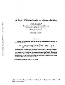
Figure 4: A non-contractible loop on a toroidal lattice with a constant frame. The single links drawn as bold lines all have transition matrices Uji = −1, whereas all other links have Uji = 1; as a consequence, the loop has a negative overall sign.

This is not, however, the case with non-contractible loops, which can take either sign. An example of a loop with negative sign is shown in fig. 4 : if we choose Uji = −1 for one complete row of links on the lattice (as in the figure) and Uji = 1 everywhere else, then any loop that encircles the lattice in the y direction passes through exactly one link with negative sign, and thus has a negative overall sign 2 . Obviously, two sign configurations are equivalent if one can transform one into the other by a sequence of local rotations Ri (2π) = −1. Because local rotations do not change the sign of any loop, a configuration with at least one loop of negative sign cannot be equivalent to a configuration that has only loops of positive sign. In other words, the two sign configurations are topologically distinct. Now, using small deformations we can easily prove that all noncontractible loops encircling the torus in the same direction must have the same sign. This means, for example, that it is sufficient to calculate the sign of just one ‘vertical’ loop (which encircles the lattice in the y direction) to know the sign of all other vertical loops. More generally, the sign of a loop is not a property of a single loop but rather of all loops in the same homotopy class, i. e. those that can be obtained from each other by a sequence of small 2

More generally, if a loop which encircles the lattice in the y direction goes back and forth having a sort of S shape, it may cross links with negative signs more than once. The number of crossings is however odd.

13

Figure 5: (Left) A lattice with toroidal boundary conditions. (Right) A lattice with the boundary conditions of a Klein bottle. The arrows indicate the directions in which the opposite edges are to be taken when joined together.

deformations. On the torus there are two independent non-trivial homotopy classes of loops (‘vertical’ and ‘horizontal’) and, therefore, four distinct possible sign configurations. These, in turn, correspond to four distinct spin structures. The statement can be generalized by observing that there are 2g independent classes of non-contractible loops on a surface with genus g, which means that there are 22g different sign configurations and thus the same number of spin structures. In particular, a lattice with spherical topology admits only one spin structure. On the other hand, on a non-orientable lattice one cannot globally define a field of orientable frames. An example of such a lattice is the so-called one-sided torus or Klein bottle, which is constructed in the same way as the standard torus but has different boundary conditions, as shown in fig. 5. It is possible to show that a frame transported along a closed path would have changed its handedness after a complete tour around the lattice. Because there does not exists a field of orientable frames, one cannot in this case define a spin structure or a Dirac operator.

4

Local frames on a random lattice

The form (10) of the Wilson action is particularly simple not only because of the simple topology of the torus, which allows for the definition of a global frame, but also because of the regular geometry of the lattice which every14

where repeats the same simple motif. On an irregular lattice, local angles and link lengths change from point to point. This must be reflected in the construction of the hopping term, which depends on these local details through the covariant derivative. To make the geometrical part of the discussion as simple as possible, and to minimize the number of local degrees of freedom of the lattice, we restrict the discussion to equilateral random triangulations. This greatly reduces the number of local degrees of freedom, making the discussion more transparent and allowing us to focus on the interesting topological part of the problem. Let us mention, however, that the presented construction can be easily generalized to the case of variable link lengths and angles. On an equilateral triangulation, the local geometry is completely encoded in the connectivity of the lattice; all other details are fixed by the simple geometry of the equilateral triangle. In particular, the deficit angle at a vertex i is determined solely by its order qi : ∆i = (6 − qi )π/6. The local curvature of the lattice is concentrated in the vertices of the triangulation. The geometry becomes singular in these points and therefore it is difficult to provide a unique definition of a tangent space at the vertices. It is more convenient to define tangent spaces at the dual points of the lattice, i. e. at the centers of the triangles. Inside each triangle the geometry is locally flat and thus naturally spans a tangent space. We therefore locate all local frames, and also all fermionic fields, at the centers of the triangles. Each point i where a field is defined has then three neighbors, each of which at the same distance from i. The vectors pointing to the neighbors are also equally spaced in the angular variable, i. e. they are separated by angles 2π/3. Before defining the fermionic fields, however, let us discuss the properties of the field of oriented orthonormal local frames on such a random triangulation. An example of a triangulation decorated with frames is shown in fig. 6. At each triangle i live two orthonormal vectors ei1 and ei2 such that eia ·eib = δab . Apart from the internal product there is also an external one ∧, which enables one to choose frames with the same handedness ei1 ∧ei2 > 0 for all triangles. Now consider two neighboring triangles i and j, each endowed with its own frame ei and ej . The interiors of the two triangles together form a flat patch of the triangulation. One can think of the two frames as being two alternative frames for the same patch. One can calculate components of our objects in either one of them, and easily recalculate them when going from one to the other. To this purpose introduce SO(2) transition matrices Uij and Uji such that : Uij Uji = 1 ,

ei = Uij ej , 15

ej = Uji ei .

(29)

k i qi =4

j U jk

Figure 6: A small piece of a random triangulation with local frames. Ujk is the transition matrix between the frames at k and j, and qi is the order of the vertex i.

One can repeat the same calculation for any pair of neighboring triangles and use it to transport a frame between any two points i1 and in along an open path C = (i1 , i2 , . . . , in ) : ein = Uin in−1 . . . Ui3 i2 Ui2 i1 ei1 = U(C) ei1 .

(30)

Since we study a theory whose content is independent of the choice of frames, we are interested in the pertinent transformation laws and in quantities invariant under local SO(2) rotations of the frames : ei → e′i = Ri ei . The object U(Cji ) = Ujk . . . Uni for any open path between i and j transforms as : U(Cji ) → U ′ (Cji) = Rj U(Cji )Ri−1 , (31) as one can see from (29). In particular, for a closed path Li beginning and ending at the same triangle i, U(Li ) transforms as U(Li ) → U ′ (Li ) = Ri U(Li )Ri−1 ,

(32)

and hence Tr U(Li ) is an invariant. Moreover, this invariant does not depend on the choice of the initial point i of the loop, and is thus a property of the loop L itself. It is a geometrical quantity related simply to the total angle R dα by which a tangent vector is rotated when transported along the loop. On a flat lattice, this angle is a multiple of 2π. On a curved lattice the 16

situation is somewhat more complicated. In particular, for an elementary loop Lq surrounding a vertex of order q, the loop invariant is 1 qπ (6 − q)π Tr U(Lq ) = cos = cos = cos ∆q (33) 2 3 3 and contains information about the deficit angle ∆q , or equivalently about the curvature at the vertex. There are various possibilities to prove this statement; the proof outlined here offers us an opportunity to introduce an auxiliary construction which will be useful throughout the remaining part of the paper, especially when we shall lift the spin connection to the spinorial representation. Recall that the information about the local geometry of the lattice is (i) stored in the form of three local unit vectors nji pointing from i to its three nearest neighbors. There is, however, another and for the problem at hand (i) more suitable way of achieving the same goal. Instead of the vectors nji (i) themselves, one can equivalently consider the rotations that connect nji to ei . To introduce the rotation matrices, we first associate an entire frame (i) with each of the three nearest neighbor vectors, treating nji as the first basis vector of each corresponding frame. The second base vector of the frame is then automatically determined by the orthonormality condition. Now we (i) (i) (i) have three particular frames nji,a = (nji,1, nji,2 ) for the three neighbors j of i. (i) (i) The frames nji can be obtained from the local frame ei by a rotation Bj : (i)

(i)

nji = Bj ei .

(34)

We refer to them as to the basic rotations at i. Now, it is convenient to decompose the connection matrices Uji into basic (i) (j) rotations Bj at i and Bi at j. Letting them act first on the frame ei , one (i) (j) obtains the frame nji . One then flip it to the frame nij using a rotation by π, which is represented by the matrix F = eǫπ . Finally, using the inverse basic rotation at j one rotates it to ej . In other words, the transition from ei to ej (and vice versa) can be done in the following three steps (see fig. 7) : (j)

(i)

(i)

ej = [Bi ]−1 F Bj ei ,

(j)

ei = [Bj ]−1 F Bi ej .

(35)

Comparison with (29) leads to : (i)

(j)

(j)

Uij = [Bj ]−1 F Bi ,

(i)

Uji = [Bi ]−1 F Bj .

(36)

One can use this decomposition to calculate the loop invariants Tr U(L) : Tr U(L) = Tr

n Y

Uik+1 ik = Tr

k=1

17

Y k

Tik

(37)

k

ej1 i

ei1

j

nji

n Figure 7: A patch of two neighboring triangles, and the three nearest neighbor vectors nij for each of them. The same information can be provided by a rotation matrix between nij and the first basis vector ej1 , shown as the flag emerging from the center of each triangle. In this example, the basic rota(j) tion Bi of frame j to the direction of its neighbor i is a rotation by 5π/3, (i) whereas the basic rotation Bj of frame i to the direction of its neighbor j is a rotation by π.

Q

where is an ordered product that runs through all vertices on the loop L = (i1 , i2 , . . . , in ) with the cyclic boundary condition in+1 = i1 and the rotation matrices π (ik ) (ik ) −1 (38) Tik ≡ Bik+1 [Bik−1 ] F = e(±)ik 3 ǫ

correspond to the turn taken by the path at the triangle ik [19]. It depends on the turn-angle, which can be either +π/3 if the path turns to the left or −π/3 if it turns to the right. In fact, on a equilateral triangulation, the sign (±)ik determines completely the turn matrix Tik at the triangle ik . It does not depend on the particular orientation of the frame, because under rotation of the frame ik the basic rotations transform as : B (ik ) → B (ik ) Rik ,

[B (ik ) ]−1 → Ri−1 [B (ik ) ]−1 k

(39)

thus leaving the combination B (ik ) [B (ik ) ]−1 in Tik intact. An elementary loop around a vertex of order q turns exactly q times in the same direction. Thus we have qπ 1 qπ (6 − q)π Tr U(Lq ) = Tr e± 3 ǫ = cos = cos . 2 3 3

as claimed in (33). 18

(40)

5

The spinorial representation

The next step is to lift the connections Uij to the spinorial representation, Uij → Uij . We continue to use the convention of denoting all rotation matrices in the spinorial representation by calligraphic letters : U → U for connections, B → B for basic frame rotations, T → T for turns and F → F for flips. The starting point of the construction is the decomposition (36). If we write it in the spinorial representation, each matrix that occurs in this equation is determined only up to a sign : eǫφ → ±eǫφ/2 (28). The idea is now to affix the spinorial representation of all matrices on the right hand side of (36) with a positive sign : B = eǫφ → B = eǫφ/2 F = eǫπ = 1 → F = eǫπ/2 = ǫ ,

(41) (42)

and keep the sign sji = ±1 as a separate variable for each link : (i)

(j)

Uij → Uij = sij [Bj ]−1 ǫ Bi ,

(j)

(i)

Uji → Uji = sji [Bi ]−1 ǫ Bj .

(43)

We demand that parallel transport of a spinor along a given link and back does not change the spinor. We see that this is indeed the case, i. e. we have Uji Uij = 1 if sji sij = −1 . (44) Using a similar calculation as the one which led to (40) one finds that in the spinorial representation the loop invariant for an elementary loop around a vertex is 1 ∆q Tr U(Lq ) = SLq · cos . (45) 2 2 where ∆q is the deficit angle, and SLq is a sign ±. The factor one-half in the argument of the cosine follows from (42). The total sign of the loop, denoted by SLq , depends on the choice of signs sij in (43) and has to be calculated. We require that the signs sij are chosen in such a way that for each elementary loop the sign SLq is positive : SLq = 1 .

(46)

Note that for q = 6 this requirement is natural, because the plaquette is flat, ∆6 = 0, and as discussed before for a flat patch the parallel transport should be trivial : U(L6 ) = 1. Thus indeed we should have SL6 = 1. Also for other q’s the requirement can be motivated. The geometry of an elementary plaquette corresponds to the geometry of a flat cone, which has a singularity 19

a

a

Figure 8: The internal geometry of a set of triangles around a vertex is the same as that around the peak of a cone : it is flat everywhere except for a single point where the curvature is concentrated in a singularity. We can determine the sign of any loop around the cone if we first regularize this singularity by ‘flattening’ the cone, and find S = +1.

at the peak. The elementary loop encircles this singularity at some distance r from the peak. One can regularize the singularity by smoothing the peak, i. e. replacing it by a differentiable surface (see fig. 8). In doing so, one deforms only a very small region within a distance of ǫ around the peak, where ǫ ≪ r. Now imagine that we shrink the loop, continuously decreasing its radius. Then Tr U(r) and ∆(r) both change continuously with r. In the limit r → 0, the loop ends up on the top of the regularized part of the geometry which is flat. Thus, again S = +1 in the limit of r → 0. This already is sufficient to have positive sign for all values of r, because in the course of continuous changing, the deficit angle ∆ was changing continuously and hence the sign S could not have jumped between negative to positive values without making U discontinuous. In other words, S must keep the value +1 for all r. Because the regularized zone can be made arbitrarily small, we assume that the triangulated lattice, which corresponds to the limit ǫ → 0, inherits the property of the regularized geometry: the sign of any elementary loop is SLq = +1 for any q. In order to enforce the constraint SLq = +1 for each plaquette, one has to establish a relation between SLq and the signs of links sji. In analogy to

20

(37), one can calculate the loop invariant in the spinorial representation as : Tr U(L) = Tr

n Y

k=1

Uik+1 ik =

Y k

sik+1 ik · Tr

Y k

Tik .

(47)

Comparing this to the result pertinent for the fundamental representation (37), one finds that an additional product of link signs appears, as expected. But there is also another source of signs hidden in (47). It has its origin in the spinorial representation of the turn matrices T → T . Surprisingly, and in contrast to the fundamental representation, the product of basic rotations depends on the position of the frame. More precisely, calculating the rotation corresponding to the turn taken by the path at ik one gets an additional sign zik : π (ik ) (ik ) −1 Tik = Bik+1 [Bik−1 ] F = zik e(±)ik 6 ǫ (48)

which was not present in the fundamental representation. The reason for the appearance of these new signs is the following: In the spinorial representation, the basic rotations are given by 1

1

Bik+1 ik = e 2 φik+1 ik ǫ ,

Bik−1 ik = e 2 φik−1 ik ǫ ,

(49)

where φik+1ik and φik−1 ik are the angles between (eik 1 , nik+1 ik ) and (eik 1 , nik−1 ik ), respectively. Therefore, we have 1

1

Tik = e 2 (φik+1 ik −φik−1 ik +π)ǫ = e 2 (∆φik +π)ǫ .

(50)

By construction, φik+1 ik and φik−1 ik both lie in the range [0, 2π). However, the difference ∆φik = φik+1 ik − φik−1 ik can lie outside this range. In general, one has ∆φik + π = ±π/3 modulo 2π, but 2π can be disregarded since e2πǫ = 1. In the spinorial representation, however, due to the factor 1/2 one has (∆φik + π)/2 = ±π/6 modulo π, and this π cannot be ignored because eπǫ = ±1. One has to calculate the exponents in (50) exactly and to find all possible values of ∆φik . There are six different cases, collected in fig. 9. The flag in each drawing represents the position of the vector eik 1 , with respect to which the angles are calculated. We call it the z-flag. For example, in the drawing (a) one has φik+1 ik ∈ [0, 2π/3) and φik−1 ik = φik+1 ik + 4π/3, which yields ∆φik = −4π/3 and thus the rotation matrix : 1

π

Tik = e 2 (−4π/3+π) = e− 6 ǫ .

(51)

In the drawing (b) one has φik+1 ik ∈ [2π/3, 4π/4) and φik−1 ik = φik+1 ik −2π/3, so that ∆φik = 2π/3 and the rotation matrix is 1

5π

π

Tik = e 2 (2π/3+π)ǫ = e 6 ǫ = −e− 6 ǫ . 21

(52)

i-1 i+1 i (a)

(b)

(c)

(d)

(e)

(f)

Figure 9: The six different possibilities for a path to cross a triangle with a marked z-flag, constructed from the two possible directions of the path (left turn or right turn) and the three possible directions of the flag. The sign of ∆φik is determined by whether or not the auxiliary line to the right of the path crosses the flag.

1

∆φik

Tik = e 2 (φik+1 ik −φik−1 ik +π) ǫ

(a) (b) (c)

−4π/3 +2π/3 +2π/3

+e−π/6 ǫ −e−π/6 ǫ −e−π/6 ǫ

(d) (e) (f)

−2π/3 +4π/3 −2π/3

+e+π/6 ǫ −e+π/6 ǫ +e+π/6 ǫ

Table 1: The difference of angles ∆φik and the turning matrix Tik in the spinorial representation for the six cases shown in fig. 9.

22

The results for all six cases (a - f) are given in table 1. Inserting them into the formula for the loop invariant (47) one obtains : Tr U(L) =

Y k

sik+1 ik · Tr

Y k

Tik =

Y k

sik+1 ik zik · Tr

Y

π

e(±)ik 6 ǫ

(53)

k

where zik is the sign of Tik . Setting : SL = −

Y

sik+1 ik zik ,

(54)

k

one finds : Tr U(L) = −SL · Tr

Y

π

e(±)ik 6 ǫ .

(55)

k

The relation (54) between the loop sign SL , the link signs s, and the z-signs can be represented graphically in a very intuitive way. The signs zik tell on which side of the path lives the z-flag. If one draws an auxiliary line, as in fig. 9, that runs along the right-hand side of the main path, then the sign zik can be determined geometrically by choosing zik = −1 if the auxiliary line crosses the z-flag and zik = +1 otherwise. Similarly, one can introduce a field of flags associated with the oriented links, and choose the sign sji = −1(+1) when the respective s-flag is (is not) crossed when one is going from i to j. Because for any given link the auxiliary path crosses the s-flag when going in one direction but not in the other, this choice leads to sji sij = −1 as required by (44). The total sign SL of the loop L is now given by the number of flags FL that are crossed by the auxiliary path : SL = (−1)1+FL .

(56)

As on the regular lattice, one can use the concept of small deformations of loops to prove some topological theorems for the signs of the loops. The fact that each elementary loop has S = +1 implies that two loops L, L′ that can be transformed into each other by a small deformation always have the same sign, SL = SL′ , because a small deformation changes the number of flags crossed by the loop by an even number (see fig. 10). Thus, we see that if all elementary loops on the lattice have positive signs, all contractible loops have positive signs SL = +1, too. Likewise, one can show that all loops belonging to the same homotopy class have the same sign. In other words, all the topological theorems we found for the regular lattice hold for the triangulated one as well. The remaining thing is to check that on a given lattice an assignment of the link signs sij , ensuring the positivity of all elementary loops signs, does always exist. That it is so for any discretized orientable 2D manifold in [10, 11]. 23

Figure 10: A small deformation of a loop on a triangulated lattice.

6

The Dirac-Wilson operator

We now have all what is needed to construct the fermionic action (19). We start by casting the formula (24) for the hopping operator Hij =

i 1h (i) 1 − nji · γ Uij 2

(57)

into a form that depends on the field of orthogonal frames through the basic rotations. One can use equation (43) to decompose the matrix Uij : (i)

(j)

Uij = sij [Bj ]−1 ǫ Bi

.

(58)

(i)

Likewise, we write the vector nji in terms of the basic rotations. By definition, the basic rotations at point i relate the direction ei1 of the frame to the directions of the links between i and its neighbors j : (i)

(i)

ei1 = [Bj ]−1 nji .

(59)

In the spinorial representation (17) one can write : (i)

(i)

(i)

nji · γ = [Bi ]−1 γ 1 Bj , 24

(60)

where γ 1 = ei1 · γ is the gamma matrix associated with the first direction of the frame. As mentioned before, the gamma matrices have the same numerical values γ 1 = σ3 , γ 2 = σ1 in each frame on the triangulation. Inserting everything into (57) we eventually obtain : 1 (i) (j) Hij = sij [Bj ]−1 [1 − γ 1 ]ǫBi , 2

(61)

which defines the hopping term in the Dirac-Wilson operator on the triangulated lattice. To calculate the basic rotations, one has to find on each triangle the three (i) angles between ei1 and the nearest neighbor vectors nji ; denote them by φj . Each is defined in the fundamental range of the rotation group, [0, 2π). Since physical quantities cannot depend on the choice of the field of frames, we are free to make the most convenient choice. Hence, we assume that in each triangle the vector ei1 points to one of the vertices. This implies that the (i) angles φj can take only one of the three possible values - π/3, π or 5π/3 which in turn makes the basic rotation matrices very simple : (i) Bj

φ

=e

(i) j ǫ 2

(i)

(i)

cj sj (i) (i) −sj cj

=

!

,

(62)

where (i) cj

√ √ (i) φj 3 3 ≡ cos = , 0, − 2 2 2

(i)

(i)

,

sj ≡ sin

φj 1 1 = , 1, 2 2 2

(63)

(i)

for φj = π/3, π, 5π/3, respectively. Inserting this explicit form of the basic rotations into (61) leads to an extremely simple formula because (1 −γ 1 )/2 is a projection matrix, which with our choice of γ 1 has only one non-vanishing element. Hence : (i) (j)

Hij = sij

(i) (j)

sj ci sj si (i) (j) (i) (j) −cj ci −cj si

!

.

(64)

In this form the Dirac-Wilson operator is easy to implement. For each pair of neighboring triangles j and i we first find the sign sji and the angles between the z-flag and the dual link ji and calculate the appropriate trigonometric functions. For example, assuming sij = 1 for the link ji in fig. 7 we have (j) (i) φi = 5π/3, φj = π. Hence : Hij =

−

√

25

3 2

1 2

0 0

!

.

(65)

The Dirac-Wilson operator is built from blocks like the above one, for each pair of indices representing neighboring triangles, and from 2×2 unit matrices for each pair of identical indices. Defining the adjacency matrix for triangles as : ( 1 if i and j are neighbors Aij = (66) 0 otherwise one can write the Dirac-Wilson operator as : Dij = −KAij Hij + δij 1 .

(67)

What are the properties of the Dirac-Wilson operator in this form? Consider the charge conjugation transformation : ψ → ψc = C ψ¯T ,

ψ¯ → ψ¯c = −ψ T C −1 ,

(68)

where the matrix C is unitary and fulfills the requirements : C −1 γ T C = −γ ,

C T = −C .

(69)

One can check that the hopping operator (61) transforms as : T −1 CHij C = Hji .

(70)

In two dimensions we can choose the standard antisymmetric matrix ε as the charge conjugation matrix, C = ε. It is convenient to use two different versions of ε, one with lower indices εαβ and one with upper indices εαβ , but with the same numerical values : ε12 = ε12 = 1 ,

εαγ εγβ = −δαβ .

(71)

One can treat ε as a simplectic form to raise or lower the spinorial indices : (ψc )α = εαβ ψ β ,

(ψc )α = ψβ εβα .

(72)

We recall that in the explicit index notation, the components of the spinor ψ¯ are denoted by ψ α and those of ψ by ψα . Furthermore, in this notation one can write : Dijαβ = εαγ [Dij ]βγ . (73) In the implicit index notation one has to distinguish between different cases, namely D for mixed indices, εD for only upper indices, and Dε for only lower indices, by displaying explicitly the action of ε. The fact that the hopping operator is constructed from a projector implies in particular, that : Hij Hji = 0 ,

Hij Uji Hij = Hij . 26

(74)

The consequence of the transformation law (70) is that :

and, furthermore, that :

T εHij ε = −Hji

(75)

(εDij )T = −εDji .

(76)

In index-explicit notation, this last equation reads : βα Dijαβ = −Dji ,

(77)

which means that the matrix Dijαβ is antisymmetric in the double indices I = (iα) and J = (jβ) : DIJ = −DJI .

7

Second-quantized theory

Quantum field theory of free Dirac fermions in a curved geometrical background represented by a triangulation T is defined by the partition function : ZT (K) =

Z Y i

β

d2 ψi d2 ψ¯i e−ψi [Dij ]α ψiβ = |D| . α

(78)

The propagator is : µ hψnν ψm i=

1 Z Y 2 −1 µ µ −ψiα [Dij ]β α ψiβ = [Dnm ]ν . d ψi d2 ψ¯i ψnν ψm e ZT (K) i

(79)

It transforms under a local change of frames ei → e′i = Ri ei as follows : µ hψnν ψm i →

D

µ

E

D

E

µ β ′ ψnν ψ ′ m = [Rn ]αν [R−1 m ]β ψnα ψm .

(80)

Let us further explore the consequences of the symmetry with respect to the charge conjugation that is encoded in the transformation law (70). Introduce two families of Majorana fermions : 1 φ1 = (ψc + ψ) , 2 1 φ2 = (ψc − ψ) , 2i

1 ¯ , φ¯1 = (ψ¯c + ψ) 2 −1 ¯ ¯ . φ¯2 = (ψc − ψ) 2i

(81)

They are charge self-conjugate : φ1c = φ1 and φ2c = φ2 . This means that the components of φ1 are not independent, likewise for φ2 . The components are related : φα = φβ εβα . (82) 27

as can be seen from (72). We skipped the family index 1, 2 in the last formula. It is convenient to express the Dirac-Wilson action in terms of the Majorana families φ1 and φ2 . Indeed, using equation (70) one finds that the two families decouple : ¯ ψ) = S(ψ,

X 1X ¯ ψi ψi − K ψ¯i Hij ψj = S(φ1 ) + S(φ2 ) 2 i hiji

where S(φ) =

X 1X¯ φi φi − K φ¯i Hij φj . 2 i hiji

(83)

(84)

¯ ψ) and S(φ) appear identical to each other, but they The two actions S(ψ, differ in the number of degrees of freedom; in the latter case, φ¯ is uniquely determined by φ. By changing the variables in the integration measure of (78) one can rewrite the partition function as a product of two identical factors : Z Y d2 φ1i d2 φ2i e−S(φ1 )−S(φ2 ) = [ZT (K)]2 (85) ZT (K) = i

where ZT (K) is the partition function for a single Majorana family : Z Y

ZT (K) =

i Z Y

=

− 21

d2 φi e

P

i

φ¯i φi +K

αβ

d2 φi e−φiα Dij

φiβ

P

hiji

φ¯i Hij φj

= Pfaff[εD] .

(86)

i

Here, εD is the antisymmetric matrix (77), which implies that the square of the Pfaffian is equal to the determinant of εD, which is in turn equal to the determinant of D. We can calculate the partition function for the Majorana fermions using the hopping parameter expansion. This leads to a geometrical interpretation of the model, as will be seen in the next section.

8

Fermionic loops

To find the hopping parameter expansion of ZT (K) let us first split the integrand into two parts : ZT (K) =

Z Y

1

¯

d2 φi e− 2 φi φi

i

Y hiji

1 + K φ¯i Hij φj

(87)

The first part is a product of independent one-point integrations with an exponential measure, whereas the second is a product over all oriented links 28

that connect neighboring points. Since we know from equations (70) and (75) that for Majorana fermions : φ¯j Hji φi = φ¯i Hij φj ,

(88)

it is convenient to rewrite the product in (87) as a product over non-oriented links (ij) : ZT (K) =

Z Y

1

¯

d2 φi e− 2 φi φi

i

Y (ij)

1 + 2K φ¯i Hij φj .

(89)

To do this, we have to require that terms like φ¯i Hij φj φ¯j Hji φi do not occur in the expansion. Actually, they vanish because of (74). The only non-vanishing integrals relevant to our problem are : Z

and

Z

1

¯

d2 φ e− 2 φφ · 1 = 1

1¯ ¯ = 1. d2 φ e− 2 φφ · (φ · φ)

(90)

(91)

These rules are used to calculate the integral of each term in the expansion : Y

(1 + 2K φ¯i Hij φj ) = 1 + 2K

(ij)

+(2K)

X (ij)

2

φ¯i Hij φj

X

(ij),(kl)

φ¯i Hij φj · φ¯k Hkl φl + . . .

(92)

Consider the quadratic term on the right hand side. If j = k then, according to (91), the integration over φj yields : X

(ij),(jl)

φ¯i Hij φj · φ¯j Hjl φl =

X

(ij),(jl)

φ¯i (Hij Hjl )φl .

(93)

Otherwise, if j 6= k, the integral vanishes. In general, one observes that the contribution of a term in the expansion (92) is non-vanishing only when all neighboring fields φj · φk belong to the same point. Integration of these terms over all fields gives : φ¯j1 Hj1 j2 Hj2 j3 · · · Hjn−1 jn φjn ,

(94)

where all ji in the chain are different. For the final integration to yield something non-vanishing one must have j1 = jn . Finally : C(L) = −Tr Hj1 j2 Hj2 j3 · · · Hjn−1 j1 . 29

(95)

This contribution can be graphically represented by a closed loop L = (j1 , j2 , . . . , jn−1 , j1 ) of length n. On the other hand, integration over a field φk associated with a vertex k that does not lie on any loop contributes a factor of 1 (90). In summary, all terms of the expansion that survive the integration (89) can be represented graphically as diagrams consisting of closed loops. These loops do not back-track or touch each other. A configuration consisting of l loops L1 , L2 , . . . , Ll with total length n = n1 + . . . + nl contributes a term (2K)n C(L1 )C(L2 ) . . . C(Ll )

(96)

to the partition function. One can calculate the contribution C(L) of a single loop L in a way similar to that used to obtain the loop invariant (47), i. e. by extracting the total sign of the loop (54) and expressing the remaining product in terms of turns at the vertices (48). The result is : C(L) = −Tr

Y k

Hik+1 ,ik = SL · Tr

Y k

1 Tik (1 − γ 1 ) 2

(97)

The difference between this expression and the one for the loop invariant (53) is that now in addition to the turn matrix a projection operator appears in the product. Inserting the explicit form of the turn matrix Ti = e±ǫπ/6 and of the projector (1 − γ 1 )/2 = (1 − σ3 )/2, one obtains : √ !n 3 . (98) C(L) = SL 2 This is again similar to the result found for the loop invariant (55), but with two differences. First, one now has SL instead of −SL . Second, in the calculation of the loop invariant the turn angles enter the result with a sign ± depending on whether the path turns left or right, whereas here the projector leaves only the cosines of the rotation matrix, which depend on √ the absolute value of the turn angle. Thus, each turn contributes a factor + 3/2 independently of its direction. Since a loop makes a turn at each vertex, the number of turns in a loop is simply equal to the loop length, which gives (98). Inserting this result into (96), one finds that the contribution of a loop configuration of total length n is : √ n Stotal · 3K , (99)

where

Stotal =

Y L

30

SL .

(100)

Figure 11: A configuration of fermionic loops.

On a lattice with spherical topology all loops L have a positive sign SL = 1 and therefore Stotal = 1 for each loop configuration. On a torus, the sign of the contribution depends on the spin structure. Assuming periodic boundary conditions in both directions (++), all loops from any non-trivial homology classes, contractible or not, have SL = 1, and again Stotal = 1 for any loop configuration. The standard notation is used here: the spin structure is referred to by the signs of independent classes of non-contractible loops. On the torus there are two classes and therefore four possibilities (ss′ ), with s, s′ = ±. Plus/minus corresponds to periodic/antiperiodic boundary condition for spinors transported along loops in this class. With anti-periodic boundary conditions in any direction - (+−), (−+), or (−−) - any non-contractible loop circling the lattice in this direction has a negative sign SL = −1. Thus, all of these three cases can produce unwanted configurations with a negative contribution to the partition function. More generally, any configuration that has an odd number of non-contractible loops circling the lattice in an anti-periodic direction has a negative total sign Stotal = −1. Yet another possible choice of boundary conditions imposes summation over all spin structures - (++), (+−), (−+), and (−−) - in the partition function. This operation is called GSO projection, and in many cases seems to be the most physical choice. Negative contributions are not a problem in this case : a configuration with an odd numbers of loops in one of the non-trivial homotopy classes, say in the first class of non-contractible loops, has Stotal = 1 for (++) and (+−), but Stotal = −1 for (−+) and (−−). The summation over all cases yields zero. More generally all ‘bad’ contributions 31

Figure 12: Domain walls versus loops on a torus. A non-contractible loop on a torus, like for instance the upper curve in the figure, cannot be a part of the domain wall configuration of Ising spins unless there is a partner curve in the same class of loops in this configuration, like for example the lower one. In general, domain-wall configurations of 2D Ising model have an even number of loops in each non-trivial class of non-contractible loops.

to the partition function cancel out in the GSO projection. Configurations with an odd number of non-contractible loops in at least one direction cannot correspond to Ising model domain wall configurations, because only an even number of these domain walls is crossed when one is performing a round trip on the lattice (see fig. 12). From this point of view, the loop cancellation in GSO projection is very physical. Before discussing this point in more detail, a more careful look at the properties of the loop signs is needed.

9

The GSO projection

As discussed in the preceding sections, the global properties of the DiracWilson operator on a two-dimensional compact manifold are closely related to the signs of the fermionic loops. Self-consistency requires a positive sign for all elementary fermionic loops, and this in turn implies a positive sign for all contractible loops. Non-contractible loops, on the other hand, are not subject to this restriction. In fact, it is the ensemble of signs of all independent non-contractible loops that defines the spin structure of the manifold. In this section, it will be shown that the sign of any loop on the lattice is uniquely determined by the signs of a minimal number of independent noncontractible loops. Stated differently: the signs of all loops on the manifold are completely encoded in the manifold’s spin structure. 32

So far, we discussed the loops without self-crossings only, for the simple reason that on a triangulation no other loops occur in the hopping parameter expansion of the Majorana-Dirac-Wilson fermions. On the other hand, we already encountered self-crossing implicitly in the calculation of the invariants Tr U(C) (47), since they can be defined on loops of any kind, including the self-crossing ones.3 For this reason, and also for the sake of completeness, we shall now discuss the signs and topological properties of loops in a general context, and restrict them to self-avoiding loops only when necessary. We require the sign of a loop to be a property of its homotopy, which means that we have to modify the definition of the sign (56) to : SL = (−1)1+FL +CLL ,

(101)

where CLL is the number of self-crossings of the loop L. Of course, for any contractible loop this must still result in a positive sign, independently of the number of self-crossings. A few examples of contractible loops with various numbers of self-crossings are shown in fig. 13. It is easy to verify that the auxiliary line running along the right hand side of the loop crosses an odd number of flags in the first two cases and an even number of flags in the last two. Let us now return to the operation that we called a ’small deformation’. So far, we have considered only deformations that do not induce self-crossings (see for example fig. 10). These deformations will be called even. It is convenient to introduce also an odd version of a small deformation, where an elementary plaquette is again used to deform the loop, but with a a selfcrossing like in fig. 14. The two kinds of small deformations differ by the orientation of the plaquette that is used to deform the loop. Neither kind changes the overall sign of the deformed loop. One can introduce equivalence classes of loops that can be obtained from each other by a sequence of small deformations. A class of loops equivalent to a loop A will be denoted by [A]. Inside this class, [A]even denotes the sub-class of loops that can be obtained from [A] by a sequence of an even number of small deformations. Let us define the loop merging operation, that acts on a set of equivalence classes of loops. Take two loops A ∈ [A] and B ∈ [B], and deform both of them smoothly until they have a common link. If this common link has 3

It is convenient to think of a self-crossing on a lattice not as a meeting at exactly one vertex, but rather as a sort of smeared overlapping that may occupy one or more links of the lattice. In particular, on a lattice with only vertices of order three, there are no exact one-vertex self-crossings; the most localized ones still occupy at least one link.

33

Figure 13: Examples of contractible loops with and without self-crossings on a square lattice. The numbers of crossed flags and self-crossings are F1 = 9, C1 = 0 for the first example; F2 = 9, C2 = 0 for the second (the flag in the center of the figure is crossed twice!) ; F3 = 8, C3 = 1 for the third; and F3 = 12, C3 = 1 for the last one. The result is a positive sign in all cases. Note that in the last three examples, the flag at the vertex in the center, where four links of the loop meet, is crossed an even number of times by the auxiliary line.

Figure 14: Even and odd versions of a ’small deformation’. In the upper figure, the two loops contain a common link of opposite orientation, causing the two versions of the link to ‘cancel out’ in the resulting deformed loop. In the lower figure, the common link has the same orientation in both loops, causing it to appear twice in the deformed loop and thus introducing a selfcrossing.

34

A

B

A

B

A·B

A·B

Figure 15: The loop merging operation. Two loops A ∈ [A] and B ∈ [B] are smoothly deformed until they share a link. They are then joined either by erasing the link or by a self-crossing, depending on the link’s relative orientation in both loops. The resulting loop belongs to a new class of loops [A · B]. an opposite orientation in both loops, erase it and form a loop out of the remaining links. Otherwise, leave the link as it is and join A and B by a self-crossing (see fig. 15). The resulting loop belongs, by definition, to a new equivalence class of loops [A · B]. The product of loop classes defined in this way has a unity element in the class of contractible loops [E], for which [A · E] = [E · A] = [A]. Counting the number of crossed flags before and after the loop merging (steps 2 and 3 in fig. 15), one finds : mod 2

F[A·B] = F[A] + F[B] + 1 + CAB ,

(102)

where CAB is the number of crossings of the loops A and B. The equation implies the law of sign composition : S[A·B] = S[A] S[B] .

(103)

Indeed, in the upper drawing in fig. 15 the loop merging does not introduce any additional self-crossing, CAB = 0, and the number of crossed flags changes by 1 modulo 2, whereas in the lower figure one additional self-crossing appears, CAB = 1, and the number of crossed flags changes by 0 modulo 2, i. e. it remaines unaltered. The factors coming from the flag count and from the number of additional self-crossings compensate each other, and the above simple composition law (103) follows. Thus, the set of equivalence classes of loops forms a group with respect to the loop merging operation. On a two-dimensional compact manifold, this group contains a minimal set of independent classes of non-contractible loops [Hi ], i = 1, . . . , 2g, where g is the genus of the manifold (see fig. 16). 35

H2g

H4

H2

H1

H2g−1

H3

Figure 16: Independent classes of non-contractible loops on a 2d manifold with genus g.

Figure 17: Loop merging on a torus. Take two loops from the classes [H1 ] and [H2 ] and smoothly deform them until they share a link, then merge them. The resulting loop [H1 · H2 ] circles the torus in both directions [H1 ] and [H2 ] simultaneously. Its sign is the product S1 · S2 . This minimal set has the nice feature that all other classes can be created from [E], [Hi ], and their inverses [Hi ]−1 by use of the loop merging operation. In other words, one can decompose any loop in terms of [E] and [Hi ], and then use equation (103) to calculate the sign of this loop as a product of signs of the Hi . Let us illustrate this with a few examples. For simplicity, denote the signs of the classes in the minimal set with Si ≡ S[Hi ] = S[Hi]−1 . Consider first a loop which goes around a torus in two distinct homotopy directions simultaneously. Such a loop can be obtained by loop merging of the classes [H1 ] and [H2 ], as shown in fig. 17. Note that the loops shown in the figure do not self-cross; nor does the resulting loop H1 · H2 . This might seem surprising at first, given that the loop merging itself introduces a crossing, CH1 H2 = 1. But indeed one can see that the original loops, even if not self-crossing, do cross each other. In general, any loop from [H1 ] always

36

H1

H3

C

Figure 18: Loop merging on a double torus. The sign of the loop in the lower figure can be calculated by observing that it can be created by a merging of the loops drawn in the upper figure. This can be done by first deforming the two loops until they have a common link, then erasing this link, and smoothly deforming the remaining loop.

crosses any loop from [H2 ] an odd number of times. In the resulting merged loop, these crossings become self-crossings, so that the product has an even number of self-crossings overall. This in turn means it can be deformed by a sequence of an even number of small deformations to a non-self-crossing loop. As a general definition, one can state that a class [A] crosses a class [B] if the number of crossings between any two representatives A and B is odd. By this definition, the classes [H1 ] and [H2 ] cross each other, as do any two of the classes [H2i−1 ] and [H2i ] shown in fig. 16. This concept will be useful in a while in the context of the GSO projection. Another example of loop merging is shown in fig. 18. The loop C in the lower drawing is obtained by merging H1 and H3 , so its sign can be calculated as the product SC = SH1 SH3 . Let us apply the sign composition law to the calculation of the partition function of Majorana fermions (89). In the hopping expansion, one generates non-self-crossing loops only. Denote the number of loops from a given class S[C] on a configuration by N[C] . Then the total sign of this configuration can be written as : N[C] Y Stotal = S[C] . (104) [C]

37

After GSO projection : Z GSO =

1 22g

X

{(±)1,...,2g }

Z ((±)1 ,(±)2 ,...,(±)2g ) ,

(105)

the total contribution of the configuration is proportional to W GSO ∼

Y [C]

1 1 + (−1)N[C] . 2

(106)

To see this, note first of all that the sum over the signs Si of the classes [Hi ] can be replaced by a sum over the signs S[C] of the classes [C] present in the configuration, since all these loops do not cross and are independent from each other. Summing over all signs S[C] means that each loop of each non-trivial class [C] occurs an equal number of times with plus and minus signs, which eventually leads to the last formula. In a sense, the action of the GSO projection factorizes into a product of independent actions for the loops of each non-trivial class on the configuration. The last equation also tells us that all configurations with an odd number of loops from any non-trivial class have a vanishing contribution to the GSO projection. Physically, this means that the projection removes all loop configurations which cannot represent domain wall configurations.

10

Topology of the Ising model

We shall consider now the Ising model with nearest neighbor interactions, focusing on the issue of the exactness of the duality transformation between the model defined on a triangulation and on its dual graph, respectively, and emphasizing the topological aspect of the duality. Furthermore, the relation between the Ising and the fermionic model will be discussed. To distinguish between a triangulation and its dual, we attach a star to symbols referring to the triangulation, while the unstared symbols refer to the dual lattice. With this convention, the partition function of the Ising spins living on the triangulation reads : (++)

ΩT∗ (β∗ ) = ΩT∗ (β∗ ) =

X

{σi∗ }

β∗

e

P

(i∗ j∗ )

σi∗ σj∗

,

(107)

where σi∗ = ±1 are spin variables located at the vertices i∗ of the triangulation. As we shall see later discussing boundary conditions for the Ising model, the partition function (107) corresponds to the partition function with the 38

Figure 19: Ising spins on the triangulated lattice, and the corresponding domain walls drawn as loops on the dual graph.

(++)

spin structure (++). Therefore we additionally denoted it by ΩT∗ (β∗ ) in the last equation. Any spin configuration on the triangulation can be graphically represented as a configuration of loops on the dual graph. Namely, for any link connecting two spin variables of opposite sign, σi∗ = −σj∗ , one can draw that link’s dual as a part of a loop. It is easy to see that the result will be loops surrounding domains of aligned spins (fig. 19). One can calculate the statistical weight of every loop configuration. For this purpose, it is convenient to rewrite the partition function as : 3/2N β∗

ΩT∗ (β∗ ) = e

X

β∗

e

{σi∗ }

P

(i∗ j∗ )

(σi∗ σj∗ −1)

,

(108)

which can be obtained from (107) by subtracting unity from the link interaction energy. Since we consider triangulations without boundaries, the numbers of links and dual links are equal, NL = NL∗ , and related to the number, N, of triangles by NL = 3/2N. The subtraction of unity in each interaction term is compensated by adding an appropriate constant factor in front of the sum in (108). The contribution to the sum of a term (σi∗ σj∗ − 1) is 0 if σi∗ = σj∗ , and 2 if σi∗ 6= σj∗ . Thus, the sum in the exponent gives twice the number of domain wall links (denoted as bold links in fig. 19), which is equal to the total length n of all loops on the configuration. Therefore : ΩT∗ (β∗ ) = 2 e3/2N β∗ 39

X {L}

e−2β∗ n ,

(109)

where the sum runs over all loop configurations on the dual graph (which are identical to the loop configurations of the fermionic model discussed in the previous section). The additional factor of 2 in front of the sum reflects the fact that each loop configuration represents two distinct spin configurations which can be obtained from each other by a simultaneous flip of all spins σi∗ → −σi∗ . For a non-spherical topology, some attention has to be paid to noncontractible loops. Consider once more a toroidal triangulation. A configuration with an odd number of non-contractible loops does not form a domain wall configuration of the Ising model and therefore does not appear in (109). The same is true of the fermionic model if we perform the GSO projection. Therefore the equivalence between the models is exact : ZTGSO (K) = 2 e−3/2N β∗ · ΩT∗ (β∗ ) , if we set

√

3K = e−2β∗ ,

(110) (111)

as can be seen by comparing (99) and (109). This statement holds for an arbitrary triangulation of a two-dimensional orientable manifold without boundary. Consider now the Ising model with spins σi living on the vertices of the dual lattice, or equivalently at the centers of the triangles of the original manifold (in other words, the spins are located at the same spots as the Majorana fields φi discussed before). The partition function reads now : ΩT (β) =

X

β

e

{σi }

P

(ij)

σi σj

.

(112)

Performing the strong coupling expansion leads to the formula : ΩT (β) = cosh(β)3/2N β

XY

(1 + σi σj tanh(β)) ,

(113)

{σi } (ij)

in analogy to the hopping parameter expansion (89) in the Majorana field theory. The integration rules for Ising spins : 1 X 1 = 1, 2 σ=±

1 X σ = 0, 2 σ=±

1 X 2 σ = 1, 2 σ=±

(114)

are completely analogous to those for the fermions (90), (91).4 4

One would see a difference with the fermion rules on a lattice Pwith vertex orders greater than three, because then one could also have terms like 1/2 σ=± σ 4 = 1, whereas the R 1 ¯ corresponding terms in the Majorana model are zero, d2 φ e− 2 φφ · φφφφ = 0. However, in our case the order of the dual lattice vertices is three by construction.

40

Thus, calculating the strong coupling expansion, one again finds a sum over the same loop configurations : ΩT (β) = (2 cosh(β))3/2N β

X

(tanh β)n .

(115)

{L}′

More precisely, for a spherical lattice the loop configurations occurring in this sum are identical to the domain wall configurations of the Ising model defined on the triangulation. However, this is not true for topologies of higher genus, where configurations with an odd number of non-contractible loops from the same homotopy class occur in the strong coupling expansion (115). This is why we have put a prime on the sum, to distinguish the set of these configurations from the set of domain walls (109). If we again take the torus as an example, we see that the sum in (115) also contains configurations with a single loop, or with an even number of loops circling the torus in the H2 -direction. This kind of loop configuration is also produced in the hopping expansion of the fermionic model if we restrict it to the spin structure with periodic boundary conditions. Thus, in this case we have : (++)

if we set

ZT

(K) = (2 cosh(β))−3/2N β · ΩT (β) √

(116)

3K = tanh(β) .

(117)

The equivalence also holds for topologies of higher genus if we choose this spin structure for the fermionic model. As expected, both Ising models are almost dual to each other. The only difference comes from topological contributions related to non-contractible loops. In fact, one can make the two models exactly equivalent by a sort of a ’GSO projection’ for the Ising field. Contrary to the projection in the fermionic model, which appears as a natural option because the model has several possible spin structures, its introduction here is somewhat artificial. Again, take the torus as an example. Originally, we have only one version of the Ising model, which corresponds to the spin structure (++) (107). Now, we attempt to define a model that can reproduce the three other structures. Let us start with the spin structure (−+), corresponding to an anti-periodic boundary condition in the first homotopy direction. On this lattice, choose a non-contractible loop circling the torus once in the second homotopy direction (see fig. 20). We call this an anti-ferromagnetic line. All links (ij) that cross this line will be called anti-ferromagnetic and denoted by (ij)− . All other links will be called ferromagnetic and denoted by (ij)+ . We define the partition function as follows : (−+) ΩT (β)

=

X

{σi }

β

e

P

(ij)+

41

σi σj −

P

(ij)−

σi σj

.

(118)

j

1 0 0 1

0 1

0 i1

Figure 20: For the dual Ising model on the torus, define an anti-ferromagnetic line in the H2 -direction as a non-contractible loop circling the torus in this direction. The Ising interaction for a given link is defined as antiferromagnetic or ferromagnetic depending on whether or not it crosses the anti-ferromagnetic line.

In the strong coupling expansion, each ferromagnetic link contributes a factor + tanh(β), and each anti-ferromagnetic link, a factor − tanh(β). Each noncontractible loop in the H1 -direction has an odd number of anti-ferromagnetic links, so its contribution will be − tanhn (β), whereas each contractible loop and each non-contractible loop in the H2 -direction has an even number of anti-ferromagnetic links, thus contributing + tanhn (β). In other words, this prescription gives exactly the same sign factors as those occurring for fermionic loops on the torus with spin structure (−+). In the same manner, one can also introduce an anti-ferromagnetic line in the H1 -direction, to produce a model corresponding to a (+−) spin structure. Finally, a model with an anti-ferromagnetic line in both directions gives us a (−−) spin structure. Summing over all four cases, one obtains a model with a partition function : ΩGSO (β) = T

1 (++) (+−) (−+) (−−) ΩT (β) + ΩT (β) + ΩT (β) + ΩT (β) , 4 (++)

(119)

which is exactly dual to the Ising model ΩT∗ (β∗ ) that has its spin variables defined on the vertices of the triangulation (107), and is equivalent to the model of Majorana fermions with GSO-projection. For a lattice size going towards infinity, the difference between Ω++ T (β) and ΩGSO (β) becomes negligible. As already explained, the difference comes T only from the non-contractible loops. These loops can be regarded as having a one-dimensional entropy, in the sense that they can be ordered by a one-dimensional index that represents their position on the lattice. Because 42

A B

Y X

Figure 21: Fermions on the honeycomb lattice.

of this, they become less and less important when the system size grows. Therefore, in the thermodynamic limit one expects an exact duality between (107) and (112) even without extending the model to the spin structures (+−), (−+), and (−−). We introduced this extension here to ensure exact duality, i. e. a one-to-one map, between the two models even for systems of finite size. Generalization of this Ising model ’GSO construction’ to higher genus topologies is straightforward. In order to simulate a spin structure with an antiperiodic boundary in a given direction Hi (see fig. 16), one simply introduces an anti-ferromagnetic line in the direction Hj that crosses Hi . Altogether, this creates 22g different spin structures.

11

Two examples

As a first example, consider the Dirac-Wilson action on a regular triangulation of the two-dimensional plane (fig. 21). The fermions live at the triangle centers, on a regular hexagonal lattice. Because the lattice is flat, we can choose a global frame, i. e. with the same directions e1 and e2 at each vertex. To fix the signs, we also choose the flag assignments, which can likewise be done in a translationally invariant way. One can easily write down the fermionic action for this model. Choose an elementary cell as in fig.21. It consists of two distinct sites : A and B. The lattice can be constructed by shifting the elementary cell by multiples i1 d1 + i2 d2 of the fundamental shift vectors d1 = n0 + n1 , d2 = n0 + n2 constructed from the the link vectors : n0 = (0, 1),

n1 =

√

3 1 , 2 2

,

43

and n2 = −

√

3 1 , 2 2

.

(120)

The components of the vectors n1 and n2 are expressed in the global frame (X, Y ) shown in the figure. The position of the cell is referred to by the double integer index i = (i1 , i2 ). With this notation the action is written as : 2 h i K XX ψ¯i+d,A (1 + nd · γ)ψi,B + ψ¯i,B (1 − nd · γ)ψi+d,A 2 i d=1 i K Xh¯ ψi,A (1 − n0 · γ)ψi,B + ψ¯i,B (1 + n0 · γ)ψi,A − 2 i i 1 Xh¯ + ψi,A ψi,A + ψ¯i,B ψi,B . (121) 2 i

S = −

Since the plane is non-compact, topological effects are not relevant. From the discussion in the previous sections we know that for Majorana fermions the model with this action is equivalent to the Ising model with spin variables living at the vertices and at temperature β∗ given by (111), and likewise to the Ising model with spins at the centers of the triangles and at temperature β given by (117). The critical temperature corresponds to the critical hopping parameter, for which the fermions become massless. This critical value is easily found to be : 1 (122) Kcr = , 3 because each vertex on the dual lattice, where the fermions are living, has three neighbors. Thus, the critical temperatures for the Ising models is : √ 1 3 1 √ β∗cr = − ln , βcr = ln( 3 + 2) , (123) 2 3 2 in agreement with the known results [23] . A second example we want to discuss shortly here is the discretization of the Majorana field coupled to two-dimensional gravity. It is well-known that the integration measure over the metric field on a two-dimensional manifold can be represented by a sum over all equilateral triangulations. If we dress each triangulation in this sum with the fermion field, we effectively obtain a theory of Majorana fermions coupled to two-dimensional gravity. This theory is given by the partition function : Z(K) =

X T

ZT (K) ,

(124)

with the sum running over all triangulations with a fixed topology. For nonspherical lattices, one should sum in addition over spin structures. We can use now the equivalence between the Majorana-Dirac-Wilson action and the Ising model to substitute, triangulation by triangulation, all 44

0

-0.2

-0.4

e∗

-0.6

-0.8

-1

-1.2

-1.4 0

0.1

0.2

β

0.3

0.4

0.5

Figure 22: Comparison of the results for the energy density of Ising field computed from MC simulations of the Ising model (line) and of the corresponding qunatity eq.(128) from MC simulations of the fermionic model (crosses). The error bars are smaller than the symbols used.

terms ZT in the sum. We again obtain an exact map between the Ising model and the model of fermions coupled to gravity. The Ising model, however, is exactly solvable [24]; in particular, the critical temperature is [25] : βcr =

1 108 ln , 2 23

β∗cr =

1 131 ln , 2 85

(125)

which means that the Majorana fermions are massless when the hopping parameter K is : √ 1 −2β∗cr 85 3 . (126) Kcr = √ e = 393 3 This, again, is an exact result. The equivalence of the two models opens the possibility of studying numerically the properties of the Dirac-Wilson operator coupled to gravity. In fact, one can use the Ising model as a generator for triangulations, and then dress the configurations with local frames and z and s flags to calculate D on each of them. Since the Dirac-Wilson operator depends on the triangulation, one gets a model of dynamical fermions interacting with the fluctuating geometry. Using the Ising model as a Monte Carlo generator for configurations is many orders of magnitude more efficient than a generator referring directly to the fermionic action, since using the latter requires calculating the Pfaffian (86) in each single Monte Carlo step, an extremely costly operation in terms of CP U time. One can easily convince oneself by simulating small systems that the two generators do indeed 45

produce the same results but differ enormously in algorithm efficiency. In fig. 22 we compare the average energy of the Ising field calculated in the two different ways : (a) directly using the Ising model : 1 e∗ = − N

*

X

(i∗ j∗ )

σi∗ σj∗

+

T

=−

1 ∂ ln ΩT∗ N ∂β∗

(127)

or (b) using the equivalence (110,111) : 3 1 ∂K ∂ ln Z 1 1 X −1 e∗ = − − = − − λ 2 N ∂β ∂K 2 2N a a T

(128)

where λa are eigenvalues of the Dirac–Wilson operator D on the given triangulation T . In the derivation of the last formula we made use of the relations : + * + * 1 ∂D −1 ∂|D|1/2 ∂ = Tr (129) ln Z = D ∂K ∂K 2 ∂K T T The two methods yield the same results. Using the trick with the Ising model as a generator of triangulations one can extend the MC simulations to larger systems in order to investigate the properties of the spectrum of the Dirac-Wilson operator on dynamical triangulations. The results of these investigations has been presented elsewhere [26]. Here let us only quote a result for the finite size scaling of the pseudocritical hopping parameter K∗ defined as the value of the hopping parameter for which a mass gap is minimal. By the mass gap we mean the center of mass of the distribution of the smallest positive eigenvalue of the Majorana-Dirac-Wilson operator εD. The numerical results can be well fitted to the finite size scaling formula : K∗ = K∞ +

a Nκ

(130)

where K∞ = 0.3756(16), and κ = 1.03(30), a = −0.9(5). The parameter K∞ corresponds to the critical value of the hopping parameter in the thermodynamic limit. As one can see it agrees with the theoretical prediction Kcr = 0.3746... given by the equation (126).

12

Conclusion

The topological properties of a fermion field on discretized two-dimensional compact manifolds were discussed at length. The exact equivalence between the model of Majorana-Wilson fermions and the Ising model was established. 46

An exact duality relation for the Ising model on a compact manifold was also found. It would be important to generalize the construction to higher–dimensional simplicial manifolds. Having done this, one would then be able to attack the problem of quantum gravity interacting with a fermionic field. So far, it has only been possible to couple integer spin fields to four-dimensional simplicial gravity [16, 18]. Such a theory is known to have problems with the continuum limit [17], which could reflect the fact that higher-dimensional gravity does not exist without a proper cocktail of matter fields coupled to it. If this were true, the addition of fermions might perhaps help solving these problems. It is straightforward to generalize parts of the construction presented in this paper to higher dimensions. In particular, one can associate with each four-dimensional simplex an orthonormal oriented frame and basic rotations, and out of them one can easily build the transition matrices and spin connections. However, the problem of lifting this construction to the half-integer representation leads to additional complications. One of the reasons is that the topological problem is by itself more complicated in four dimensions. The question of whether a manifold admits a spin structure, which is equivalent to the question of whether it is possible to define globally a Dirac operator on it, is in general related to the existence of a non-trivial second Stiffel-Witney form [20, 21]. For two- and threedimensional manifolds, this reduces to the orientability question. In four dimensions, however, there are manifolds, like for example the projective space CP (C 2 ), which are orientable but possess a non-trivial Stiffel-Witney form, and thus do not admit any spin structure. In an attempt of extending our construction to a higher dimensional manifold not admitting any spin structure, the topological obstruction would manifest itself as the impossibility to adjust the local degrees of freedom so as to assign positive signs to all elementary plaquettes.

Acknowledgments We thank Joachim Tabaczek for many discussions. This work was supported in part by the EC IHP grant HPRN-CT-1999-00161 and by the Polish Government Project (KBN) 2P03B 01917.

References 47

[1] L. Onsager, Phys. Rev. 65 (1944) 117. [2] E.H. Lieb, D.C. Mattis and T.D. Schultz, Rev. Mod. Phys. 36 (1964) 407 [3] P. Pfeuty, Annals of Phys. 67 (1970) 79. [4] V. Popov, Functional integrals in quantum field theory and statistical physics Kluwer Academic Publ. 1983. [5] M.A. Bershadsky and A.A. Migdal, Phys. Lett. B174 (1986) 393. [6] N.H. Christ, R. Friedberg and T.D. Lee Nucl. Phys. B202 (1982) 89, [7] N.H. Christ, R. Friedberg and T.D. Lee Nucl. Phys. B210 (1982) 310, [8] N.H. Christ, R. Friedberg and T.D. Lee Nucl. Phys. B210 (1982) 337. [9] H.-C. Ren, Nucl. Phys. B301 (1988) 661. [10] Z. Burda, J. Jurkiewicz and A. Krzywicki, Phys.Rev.D60 (1999) 105029. [11] Z. Burda, J. Jurkiewicz and A. Krzywicki, Nucl. Phys. Proc. Suppl. 83 (2000) 742. [12] F. Gliozzi, J. Scherk and D. Olive, Nucl.Phys.B122 (1977) 253. [13] M.B. Green, J.H. Schwarz and E. Witten, String theory, Cambridge University Press 1987. [14] F. David, Nucl.Phys. B257 (1985) 45. [15] V.A. Kazakov, I.K. Kostov and A.A. Migdal Phys.Lett. B157 (1985) 295. [16] F. David, Simplicial Quantum Gravity and Random Lattices, Les Houches Summer School 1992 Proceedings, hep-th/9303127. [17] P. Bialas, Z. Burda, A. Krzywicki and B. Petersson. Nucl.Phys. B472 (1996) 293. [18] S. Bilke, Z. Burda, A. Krzywicki, B. Petersson, J. Tabaczek, and G. Thorleifsson, Phys.Lett. B418 (1988) 266. [19] M. Kac and J.C. Ward, Phys.Rev. 88 (1952) 1332.

48

[20] Y. Chocquet-Bruhat’s and C. DeWitt-Morette Analysis, Manifolds and Physics, Part II;, North-Holland 1989. [21] T. Eguchi, P. B. Gilkey and A. J. Hanson, Phys. Rept. 66 (1980) 213. [22] K. Wilson, Phys.Rev. D10 (1974) 2445. [23] R. J. Baxter, Exactly Solved Models in Statistical Mechanics, Academic Press 1982. [24] V.A. Kazakov, Phys. Lett. A119 (1986) 140. [25] Z. Burda and J. Jurkiewicz, Acta Phys. Polon. B20 (1989) 949. [26] L. Bogacz, Z. Burda, C. Petersen, and B. Petersson, e-Print Archive: hep-lat/0107015

49

6

yy

4

2

0 0

0.2

0.4

0.6 xx

0.8

1

6 5

yy

4 3 2 1 0 0

0.2

0.4

0.6 xx

0.8

1

0.5 0.3

yy

0.1 -0.1 -0.3 -0.5 0

0.2

0.4

0.6 xx

0.8

1

6

5

yy

4

3

2

1

0 0

0.2

0.4

0.6 xx

0.8

1

1.2

Dirac operator and Ising model on a compact 2D random lattice

Dirac operator and Ising model on a compact 2D random lattice

Suggest Documents

A Short visit on Ising 2D Model

A Spin-3/2 Ising Model on a Square Lattice

ZERO-TEMPERATURE 2D STOCHASTIC ISING MODEL AND

Magnetic susceptibility of the 2D Ising model on a finite lattice

Overlap Dirac operator at nonzero chemical potential and random ...

Spectral Properties of the Wilson Dirac Operator and random matrix ...

Complex-Temperature Properties of the Ising Model on 2D ...

Droplet Motion for the Conservative 2D Ising Lattice Gas Dynamics ...

Ising model on hyperbolic lattice studied by corner transfer matrix ...

Cutoff for the Ising model on the lattice

Dynamical Properties of Random Field Ising Model

The antiferromagnetic Ising model on the swedenborgite lattice

Chaos in the Random Field Ising Model

Cutoff for the Ising model on the lattice

Universal fluctuations in spectra of the lattice Dirac operator

Self-averaging in the random 2D Ising ferromagnet

Random Matrices in 2D, Laplacian Growth and Operator Theory

Lattice Ising model in a field: E8 scattering theory

The Overlap Dirac Operator

large deviations and continuum limit in the 2d ising model

Percolation and number of phases in the 2D Ising model

Ising Problem on Simple Cubic Lattice Abstract

K-homology class of the Dirac operator on a compact quantum group

On the twisted Dirac operator - SSMR