Overview of Parallel Photo-realistic Graphics - Semantic Scholar

EUROGRAPHICS ’98

STAR – State of The Art Report

Overview of Parallel Photo-realistic Graphics E. Reinhard† , A. G. Chalmers† and F. W. Jansen‡

Abstract Global illumination is an area of research which tries to develop algorithms and methods to render images of artificial models or worlds as realistically as possible. Such algorithms are known for their unpredictable data accesses and their high computational complexity. Rendering a single high quality image may take several hours, or even days. For this reason parallel processing must be considered as a viable option to compute images in a reasonable time. The nature of data access patterns and often the sheer size of the scene to be rendered, means that a straightforward parallelisation, if one exists, may not always lead to good performance. This holds for all three rendering techniques considered in this report: ray tracing, radiosity and particle tracing.

1. Introduction Physically correct rendering of artificial scenes requires the simulation of light behaviour. Such simulations are computationally very expensive, which means that a good simulation may take between a couple of hours to several days. The best lighting simulation algorithms to date are ray tracing 109 , radiosity 29 and particle tracing 70 . These algorithms differ in the way the light paths are approximated. This means that the obtainable lighting effects differ from algorithm to algorithm. As pointed out by Kajiya 47 , all rendering algorithms aim to model the same lighting behaviour, i.e. light scattering off various types of surfaces, and hence try to solve the same equation, termed the rendering equation. Following the notation adopted by Shirley 89 , the rendering equation is formulated as: Lo (x; Θo ) = Le (x; Θo )+ (1) Z 0 0 cos Θ dA v(x; x0 ) fr (x; Θ0o ; Θo )Lo (x0 ; Θ0o ) cos Θi 0 o 2 kx , xk allx 0

This equation simply states that the outgoing radiance Lo at surface point x in direction Θo is equal to the emitted radiance Le plus the incoming radiance from all points x0 reflected into direction Θo . In this equation, v(x; x0 ) is a visibility term, being 1 if x0 is visible from surface point x and 0

† Dept. of Computer Science, University of Bristol, UK ‡ Faculty of Information Technology and Systems, Delft University of Technology, The Netherlands

otherwise. The material properties of surface point x are represented in the bi-directional reflection distribution function (BRDF) fr (x; Θ0o ; Θo ), which returns the amount of radiance reflected into direction Θo as function of incident radiance from direction Θ0o . The cosine terms translate surface points in the scene into projected solid angles. The rendering equation is an approximation to Maxwell’s equation for electromagnetics 47 and therefore does not model all optical phenomena. For example, it does not include diffraction and it also assumes that the media inbetween surfaces do not scatter light. This means that participating media, such as smoke, clouds, mist and fire are not accounted for without extending the above formulation. There are two reasons for the complexity of physically correct rendering algorithms. One stems from the fact that the quantity to be computed, Lo is part of the integral in equation 1, turning the rendering equation into a recursive integral equation. The other is that, although fixed, the integration domain can be arbitrarily complex. Recursive integral equations with fixed integration domains are called Fredholm equations of the second kind and have to be solved numerically 18 . Ray tracing (section 3), radiosity (sections 4 to 7) and particle tracing (section 8) are examples of such numerical methods approximating the rendering equation. Ray tracing approximates this Fredholm equation by means of (Monte Carlo) sampling from the eye point, particle tracing by sampling from the light sources. Radiosity is a finite element method for approximating energy exchange between surfaces in a scene. To speed up these algorithms, many different schemes have been proposed, of which parallel processing is one. To

Reinhard et al. / Overview of Parallel Photo-realistic Graphics

succesfully implement a rendering algorithm a number of issues must be addressed. First of all, a decision must be made whether the algorithm is going to be decomposed into separate functional parts (algorithmic decomposition), or if identical programs are going to be executed on different parts of the data (domain decomposition). The latter tends to be more suitable for parallel rendering purposes and is certainly the method that is most used nowadays. This report therefore concentrates on domain decomposition methods. Second, the type of parallel hardware must be considered. If no dedicated parallel hardware is available, clusters of workstations may be used (distributed processing), otherwise with dedicated multiprocessors a decision must be made whether to use shared or distributed memory machines. Shared memory systems have the advantage of simplicity of programming, as all processors address the same pool of data. On the other hand, this is also a disadvantage, because memory access may become a bottleneck when a large number of processors are connected together. Distributed memory systems are theoretically more scalable, but in practice moving data from processor to processor is a costly affair, limiting the scalability of the system. Most parallel rendering algorithms are implemented on distributed memory systems, with a few notable exceptions. Third, tasks need to be identified and the appropriate data for them selected. Managing which tasks are going to be executed by which processors and if and how data is going to be moved around between various processors are important design decisions which directly affect performance of the resulting parallel system. Improper task and data management may lead to idle time, for example because the workload is unevenly distributed between processors (load imbalance) or because of the time delay when data needs to be fetched from remote processors. Excessive data or task communication between processors is another common performance degrading effect. Choreographing tasks and data such that all processors have sufficient work all the time, while ensuring that the data needed to complete all tasks is available at the right moments in time, are the main issues in parallel processing. Generally, three different types of task scheduling are distinguished, which are data parallel, data driven and demand driven scheduling. If data is distributed across a number of processors, then data parallel scheduling implies that tasks are executed with the processors that hold the data required for those tasks. If some data items are unavailable at one processor, the task is migrated to the processor that holds these data items. Very large data sets can be processed in this way, because the problem size does not depend on the size of a single processor’s memory. In data driven scheduling, all tasks are distributed over the processors before the computations start. Scheduling is extremely simple, but data management is more difficult. Data either has to be replicated, or data fetches may occur, penal-

ising performance. Another disadvantage is that the workload associated with each task (and thus each processor) is unknown, and therefore load imbalances may occur. Demand driven scheduling is generally most succesful in avoiding load imbalances, because work is distributed on demand. Whenever a processor finishes a task, it requests a new task from a master processor. Data management is similar to data driven scheduling, which means that demand driven scheduling, with data replicated across the processors, leads to the best performance. Demand driven and data parallel types of scheduling are sometimes combined into a hybrid scheduling algorithm. Each processor then stores part of the data. Whenever data accesses are unpredictable, or a large amount of data is required to complete a task, these tasks are handled in data parallel fashion. If a task requires a relatively small amount of data, which can be determined before the task is executed, then this task can be executed in demand driven fashion. By scheduling such tasks with processors that have a low workload, load imbalances due to data parallel scheduling can be minimised, while at the same time very large problems can be solved. For really complex scenes, the above scheduling approach may loose efficiency because of loss of data and cache coherence, in particular for the demand-driven scheduling. Recently, several techniques have been developed to improve data locality, either by replacing complex objects by simpler approximations or by reordering computations. Similar data management strategies have been proposed to reduce the amount of task communication in data parallel approaches. This report is structured as follows. Section 2 discusses the overheads which are invariably associated with parallel processing and which must be dealt with in any parallel rendering system. In section 3 ray tracing and its parallel variants are explained, while the same is done for radiosity in section 4 and for stochastic rendering in section 8. Issues pertaining to preserving and exploiting coherence and data locality are discussed in section 9. Finally, this paper is rounded up with a discussion in section 10. 2. Realisation penalties If the same processor is used in both the sequential and parallel implementation of a problem, then we should expect, that the time to solve the problem decreases as more processors are added. The best we can reasonably hope for is that two processors will solve the problem twice as quickly, three processors three times faster, and n processors, n times faster. If n is sufficiently large then by this process, we should expect our large scale parallel implementation to produce the answer in a tiny fraction of the sequential computation. However, in reality we are unlikely to achieve these optimised times as the number of processors is increased. A


more realistic scenario is that the time taken to solve the example problem on the parallel system initially decreases up to a certain number of processing elements. Beyond this point, adding more processors actually leads to an increase in computation time. Failure to achieve the optimum solution time means that the parallel solution has suffered some form of realisation penalty 9 . A realisation penalty can arise from the algorithm itself or from its implementation. The algorithmic penalty stems from the very nature of the algorithm selected for parallel processing. The more inherently sequential the algorithm, the less likely the algorithm will be a good candidate for parallel processing. It has been shown, albeit not conclusively, that the more experience the writer of the parallel algorithm has in sequential algorithms, the less parallelism that algorithm is likely to exhibit 10 . The sequential nature of an algorithm and its implicit data dependencies will translate, in the domain decomposition approach, to a requirement to synchronise the processing elements at certain points in the algorithm. This can result in processing elements standing idle awaiting messages from other processing elements. A further algorithmic penalty may also come about from the need to reconstruct sequentially the results generated by the individual processors into an overall result for the computation. Solving the same problem twice as fast on two processing elements implies that those two processing elements must spend 100% of their time on computation. We know that a parallel implementation requires some form of communication. The time a processing element is forced to spend on communication will naturally impinge on the time a processor has for computation. Any time that a processor cannot spend doing useful computation is an implementation penalty. Implementation penalties are thus caused by: The need to communicate As mentioned above, in a multiprocessor system, processing elements need to communicate. This communication may not only be that which is necessary for a processing element’s own actions, but in some architectures, a processing element may also have to act as a intermediate for other processing elements’ communication. Idle time Idle time is any period of time when a processing element is available to perform some useful computation, but is unable to do so because either there is no work locally available, or its current task is suspended awaiting a synchronisation signal, or a data item which has yet to arrive. The computation to communication ratio within the system will determine how much time is available to fetch a task before the current one is completed. A load imbalance is said to exist if some processing elements still have tasks to complete, while the others do not. The domain decomposition approach means that the problem domain is divided amongst the processing elements

in some fashion. If a processing element requires a data item that is not available locally, then this must be fetched from some other processing element within the system. If the processing element is unable to perform other useful computation while this fetch is being performed, for example by means of multi-threading, then the processing element is said to be idle. Concurrent communication, data management and task management activity Implementing each of a processing element’s activities as a separate concurrent process on the same processor, means that the physical processor has to be shared. When another process other than the application process is scheduled then the processing element is not performing useful computation even though its current activity is necessary for the parallel implementation. The fundamental goal of parallel processing is to minimise the implementation penalty. While this penalty can never be removed, intelligent communication, data management and task scheduling strategies can avoid idle time and significantly reduce the impact of the need to communicate.

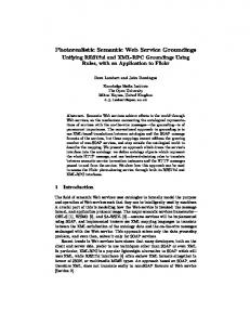
3. Ray tracing The basic ray tracing algorithm 109 follows, for each pixel of the image, one or more rays into the scene. If such a primary ray hits an object, the light intensity of that object is assigned to the corresponding pixel. From the intersection point of the ray and the object, new rays are spawned towards each of the light sources (figure 1). When these shadow rays intersect other objects between the intersection point and the light sources, intersection point is in shadow, and if the light sources are hit directly, the intersection point was directly lit. Mirroring reflection and transparency may be modelled similarly by shooting new rays into the reflected and/or transmitted directions (figure 1). These reflection and transparency rays are treated in exactly the same way as primary rays. Hence, ray tracing is a recursive algorithm. In terms of the rendering equation, ray tracing is defined as 53 : Lo (x; Θo ) = Le (x; Θo )+ Z v(x; xl ) fr;d (x)Le (xl ; Θ0o ) cos Θl dωl + ∑ L

Z

2

allxi L

2

Θs Ωs

fr;s (x; Θs ; Θo )L(xs ; Θs ) cos Θs dωs +

ρd La (x) Here, the second term on the right hand side computes the direct contribution of the light sources L. The visibility term is evaluated by casting shadow rays towards the light sources. The specular contribution is computed by evaluating the third term. If the specular component (the same holds


Shadow rays Shadow rays

Screen

Primary ray Eye point Reflection ray Figure 1: Modelling reflection and shadowing.

for transparency) intersects a surface, this equation is evaluated recursively. As normally no diffuse interreflection is computed in ray tracing, the ambient component is approximated by a constant, the fourth term.

ure 1 is one such example of a complex scene in which a large concentration of objects is used to model the musical equipment and the couches. The floor and the walls, however, consist of just a few objects.

This recursive process has to be carried out for each individual pixel separately. A typical image therefore costs at least a million primary rays and a multiple of that in the form of shadow rays and reflection and transparency rays. The most expensive parts of the algorithm are the visibility calculations. For each ray, the object that intersected the ray first, must be determined. To do this, a potentially large number of objects will have to be intersected with each ray.

Adaptive spatial subdivisions, such as the octree 27 and the bintree are better suited for complex scenes. Being tree structures, space is recursively subdivided into two (bintree) or eight (octree) cells whenever the number of objects in a cell is above a given threshold and the maximum tree depth is not yet reached. The cells are smaller in areas of high object concentration, but the number of objects in each cell should be more or less the same. The cost of intersecting a ray with the objects in a cell is therefore nearly the same for all cells in the tree.

One of the first and arguably one of the most obvious optimisations is to spatially sort the objects as a pre-process, so that for each ray instead of intersecting all the objects in the scene, only a small subset of the objects need to be tested. Sorting techniques of this kind are commonly known as spatial subdivision techniques 28 . All rendering algorithms that rely on ray casting to test visibility, benefit from spatial subdivisions. The simplest of all spatial subdivisions is the grid, which subdivides the scene into a number cells (or voxels) of equal size. Tracing a ray is now performed in two steps. First each ray intersects a number of cells, and these must be determined. This is called ray traversal. In the second step objects contained within these cells are intersected. Once an intersection in one cell is found, subsequent cells are not traversed anyfurther. The objects in the cells that are not traversed, are therefore not tested at all. Although the grid is simple to implement and cheap to traverse, it does not adapt very well to the quirks of the particular model being rendered. Complex models usually concentrate a large number of objects in a few relatively small areas, whereas the rest of the scene is virtually empty. Fig-

Experiments have shown that as a rule of thumb, the number of cells in a spatial subdivision structure should be of the same order as the number of objects N in the scene 78 . Given this assumption, an upper bound for the cost (in seconds) of tracing a single ray through the scene for the three spatial subdivision structures is derived as follows 80 : Grid The number of grid cells is N, so that in each of the orthogonal directions x, y and z, the number of cells will p be 3 N. A ray travelling linearly through the structure will therefore cost T

= =

p 3

p

N (Tcell + Tint ) 3

O( N )

In this and the following equations Tcell is the time it takes to traverse a single cell and Tint is the time it takes on average to intersect a single object. Bintree Considering a balanced bintree with N leaf cells,


the height of the tree will be h, where 2h = N. The number h of cells traversed by a single ray is then O(2 3 ), giving T

= = =

h

p

2 3 (Tcell + Tint ) 3

p

N (Tcell + Tint ) 3

O( N )

Octree In a balanced octree with N leaf cells, the height is h, where 8h = N. A ray traversing such an octree intersects O(2h ) cells: T

= = =

2h (Tcell + Tint )

p 3

p

N (Tcell + Tint ) 3

O( N )

Although the asymptotic behaviour of these three spatial subdivision techniques are the same, in practice differences may occur between the grid and the tree structures due to the grid’s inability to adapt to the distribution of data in the scene. Spatial subdivision techniques have reduced thepnumber of intersection tests dramatically from O(N ) to O( 3 N ), but a very large number of intersection tests is still required due to the sheer number of rays being traced and due to the complexity of the scenes that has only increased over the years. Other sorting mechanisms that improve the speed of rendering, such as bounding box strategies, exist, but differ only in the fact that objects are now bounded by simple shapes that need not be in a regular structure. This means that bounding spheres or bounding boxes may overlap and may be of arbitrary size. The optimisation is due to the fact that intersecting a ray with such a simple shape is often much cheaper than intersecting with the more complex geometry it encapsulates. Bounding spheres or boxes may be ordered in a hierarchy as well, leading to a tree structure that removes the need to test all the bounding shapes for each ray. Because bounding boxes (and spheres) are quite similar to spatial subdivision techniques, their improved adaptability to the scene and their possibly more expensive ray traversal cost being the differences, these techniques are not considered any further. The reduction in intersection tests is of the same order as for spatial subdivision techniques. As other optimisations that significantly reduce the time complexity of ray tracing are not imminent, the most viable route to improve execution times is to exploit parallel processing.

data used during the computation is read, but not modified, the data could easily be duplicated across the available processors. This would then lead to the simplest possible parallel implementation of a ray tracing algorithm. The only issue left to be addressed is that of load balancing. Superficially, ray tracing does not seem to present any great difficulties for parallel processing. However, in massively parallel applications, duplicating data across processors is very wasteful and limits the problem size to that of the memory available with each processor. When the scene does not fit into a single processors memory, suddenly the problem of parallelising ray tracing becomes a lot more interesting and the following sections address the issues involved. Three different types of scheduling have been tried on ray tracing, which are the demand driven, the data parallel and the hybrid scheduling approach. They are discussed in sections 3.2 through 3.4. 3.2. Demand driven ray tracing The most obvious parallel implementation of ray tracing would simply replicate all the data with each processor and subdivide the screen into a number of disjunct regions 67 31 73 32 33 8 60 103 42 or adaptively subdivide the screen and workload 65 66 . Each processor then renders a number of regions using the unaltered sequential version of the ray tracing algorithm, until the whole image is completed. ;

;

;

;

;

;

;

;

;

Tasks can be distributed before the computation begins 42 . This is sometimes referred to as a data driven approach. Communication is minimal, as only completed subimages need to be transferred to file. However, load imbalances may occur due to differing complexities associated with different areas of the image (see figure 2). Areas of high complexity

Areas of low complexity

3.1. Parallel ray tracing The object of parallel processing is to find a number of preferably independent tasks and execute these tasks on different processors. Because in ray tracing the computation of one pixel is completely independent of any other pixel, this algorithm lends itself very well to parallel processing. As the

Figure 2: Different areas of the image have different complexities. To actively balance the workload, tasks may be distributed


at run-time by a master processor. Whenever a processor finishes a subimage, it asks the master processor for a new task (figure 3). In terms of parallel processing, this is called the demand driven approach. In computer graphics terms this would be called a screen space subdivision. The speed-ups to be expected with this type of parallelism are near linear, as the overhead introduced is minimal. Because the algorithm itself is sequential as well, this algorithm falls in the class of embarrassingly parallel algorithms. Slave 1 Slave 2 Slave 3

Slave 4

Master processor Task request Task Pixel data Figure 3: Demand driven ray tracing. Each processor requests a task from the master processor. When the master receives a requests, it sends a task to the requesting processor. After this processor finishes its task, it sends the resulting pixel data to the master for collation and requests a new task. Communication is generally not a major problem with this type of parallel ray tracing. After finishing a task, a processor may request a new task from a master processor. This involves sending a message to the master, which in turn will send a message back. The other communication that will occur is that of writing the partial images to either the frame buffer or to a mass storage device. Load balancing is achieved dynamically by only sending new tasks to processors that have just become idle. The biggest problems occur right at the beginning of the computation, where each processor is waiting for a task, and at the end of the computation, when some processors are finishing their tasks while others have already finished. One way of minimising load imbalances would be task stealing, where tasks are migrated from overloaded processors to ones that have just become idle 3 . In order to facilitate load balancing, it would be advantageous if each task would take approximately the same amount of computer cycles. In a screen space subdivision based ray tracer, the complexity of a task depends strongly

on the number of objects that are visible in its region (figure 2). Various methods exist to balance the workload. The left image in figure 4 shows a single task per processor approach. This is likely to suffer from load imbalances as clearly the complexity for each of the tasks is different. The middle image shows a good practical solution by having multiple smaller regions per processor. This is likely to give smaller, but still significant, load imbalances at the end of the computation. Finally, the right image in figure 4 shows how each region may be adapted in size to create a roughly similar workload for each of the regions. Profiling by subsampling the image to determine the relative workloads of different areas of the image would be necessary (and may also be used to create a suitable spatial subdivision, should the scene be distributed over the processors 74 ). Unfortunately, parallel implementations based on image space subdivisions normally assume that the local memory of each processor is large enough to hold the entire scene. If this is the case, then this is also the best possible way to parallelise a ray tracing algorithm. Shared memory (or virtual shared memory) architectures would best adopt this strategy too, because good speed-ups can be obtained using highly optimised ray tracers 55 92 48 . It has the additional advantage that the code hardly needs any rewriting to go from a sequential to a parallel implementation. ;

;

However, if very large models need to be rendered on distributed memory machines or on clusters of workstations, or if the complexity of the lighting model increases, the storage requirements will increase accordingly. It may then become impossible to run this embarrassingly parallel algorithm efficiently and other strategies will have to be found. An important consequence is that the scene data will have to be distributed. Data access will incur different costs depending on whether the data is stored locally or with a remote processor. It suddenly becomes very important to store frequently accessed data locally, while less frequently used data may be kept at remote processors. If the above screen space subdivision is to be maintained, caching techniques may be helpful to reduce the number of remote data accesses. The unpredictable nature of data access patterns that ray tracing exhibits, makes cache design a non-trivial task 31 33 . ;

However, for certain classes of rays, cache design can be made a little easier by exploiting coherence (also called data locality). This is accomplished by observing the fact that sometimes the order in which data accesses are made are not completely random, but somewhat predictable. Different kinds of coherence are distinguished in parallel rendering, the most important of which are: Object coherence Objects consist of separate connected pieces bounded in space and distinct objects are disjoint in space. This is the main form of coherence; the others are derived from object coherence 99 . Spatial subdivision


1

2

2

2

1

4

3

2

1

3

4

3

1

2

1

4

3 3

2

4

4

2

2 1

a. Static load balancing

1

1

4

3

b. Dynamic load balancing

c. Dynamic load balancing with adaptive regions

Figure 4: Image space subdivision for four processors. (a) One subregion per processor. (b) Multiple regions per processor. (c) Multiple regions per processor, but each region should bring about approximately the same workload.

techniques, such as grids, octrees and bintrees directly exploit this form of coherence, which explains their success. Image coherence When a coherent model is projected onto a screen, the resulting image should exhibit local constancy as well. This was effectively exploited in 108 . Ray coherence Rays that start at the same point and travel into similar directions, are likely to intersect the same objects. An example of ray coherence is given in figure 5, where most of the plants do not intersect the viewing frustum. Only a small percentage of the plants in this scene are needed to intersect all of the primary rays drawn into it.

Viewing frustum

Eye Point

Figure 5: Ray coherence: the rays depicted intersect only a small number of objects.

For ray tracing, ray coherence is easily exploited for bundles of primary rays and bundles of shadow rays (assuming that area light sources are used). It is possible to select the data necessary for all of these rays by intersecting a bounding pyramid with a spatial subdivision structure 16 . The resulting list of voxels can then be communicated to the processor requesting the data.

3.3. Data parallel ray tracing A different approach to rendering scenes that do not fit into a single processor’s memory, is called data parallel rendering. In this case, the data is distributed amongst the processors. Each processor will own a subset of the scene database and trace rays only when they pass through its own subspace 12 50 51 6 31 74 43 94 72 104 105 49 79 . If a processor detects an intersection in its own subspace, it will spawn secondary rays as usual. Shading is normally performed by the processor that spawned the ray. In the example in figure 6, all primary rays are spawned by processor 7. The primary ray drawn in this image intersects a chair, which is detected by processor 2 and a secondary reflection ray is spawned, as well as a number of shadow rays. These rays are terminated respectively by processors 1, 3 and 5. The shading results of these processors are returned to processor 2, which will assemble the results and shade the primary ray. This shading result is subsequently sent back to processor 7, which will eventually write the pixel to screen or file. ;

;

;

;

;

;

;

;

;

;

;

;

In order to exploit coherence between data accesses as much as possible, usually some spatial subdivision is used to decide which parts of the scene are stored with which processor. In its simplest form, the data is distributed according to a uniform distribution (see figure 7a). Each processor will hold one or more equal sized voxels 12 72 104 105 79 . Having just one voxel per processor allows the data decomposition to be nicely mapped onto a 2D or 3D grid topology. However, since the number of objects may vary dramatically from voxel to voxel, the cost of tracing a ray through each of these voxels will vary and therefore this approach may lead to severe load imbalances. ;

;

;

;

A second, and more difficult problem to address, is the fact that the number of rays passing through each voxel is likely to vary. Certain parts of the scene attract more rays than other parts. This has mainly to do with the view point


1

2

4

3

Shadow rays

Primary ray 6

5

7

8 Viewing frustum

Reflection ray Spatial subdivision Figure 6: Tracing and shading in a data parallel configuration.

and the location of the light sources. Both the variations in cost per ray and the number of rays passing through each voxel indicate that having multiple voxels per processor is a good option, as it is likely to reduce the impact of load imbalances. Another approach is to use a hierarchical spatial subdivision, such as an octree 50 51 31 77 , bintree (see figures 7b and 7c) or hierarchical grids 94 and subdivide the scene according to some cost criterion. Three cost criteria are discussed by Salmon and Goldsmith 87 : ;

;

;

the data should be distributed over the processors such that the computational load generated at each processor is roughly the same. The memory requirements should be similar for all processors as well. Finally, the communication cost incurred by the chosen data distribution should be minimised.

Unfortunately, in practice it is very difficult to meet all three criteria. Therefore, usually a simple criterion is used, such as splitting off subtrees such that the number of objects in each subtree is roughly the same. This way at least the cost for tracing a single ray will be the same for all processors. Also, storage requirements are evenly spread across all processors. A method for estimating the cost per ray on a per voxel basis is presented in 80 . Memory permitting, a certain degree of data duplication may be very helpful as a means of reducing load imbalances. For example, data residing near light sources may be duplicated with some or all processors or data from neighbouring processors maybe stored locally 94 79 . ;

In order to address the second problem, such that each processor will handle roughly the same number of ray tasks,

profiling may be used to achieve static load balancing 74 43 . This method attempts to equalise both the cost per ray and the number of rays over all processors. It is expected to outperform other static load balancing techniques at the cost of an extra pre-processing step. ;

If such a pre-processing step is to be avoided, the load in a data parallel system could also be dynamically balanced. This involves dynamic redistribution of data 17 . The idea is to move data from heavily loaded processors to their neighbours, provided that these have a lighter workload. This could be accomplished by shifting the voxel boundaries. Alternatively, the objects may be randomly distributed over the processors (and thus not according to some spatial subdivision) 49 . A ray will then have to be passed from processor to processor until it has visited all the processors. If the network topology is ring based, communication could be pipelined and remains local. Load balancing can be achieved by simply moving some objects along the pipeline from a heavily loaded processor to a less busy processor. In general, the problem with data redistribution is that data accesses are highly irregular; both in space and in time. Tuning such a system is therefore very difficult. If data is redistributed too often, the data communication between processors becomes the dominant factor. If data is not redistributed often enough, a suboptimal load balance is achieved. In summary, data parallel ray tracing systems allow large scenes to be distributed over the processors’ local memories, but tend to suffer from load imbalances; a problem which is difficult to solve either with static or dynamic load balancing schemes. Efficiency thus tends to be low in such systems.


1

5

2

3

4

6

7

8

;

Grid 1

2

4

5

6

7

8

3

1

1

3

2

Octree

3

4

5

6

7

8

6

2

4 5

7

8

1 Bintree

cessors: each processor being capable of handling both types of task 88 46 44 79 . The data parallel part of the algorithm then creates a basic, albeit uneven load. Tasks that are not computationally very intensive but require access to a large amount of data are ideally suited for data parallel execution.

4

3

2

Figure 7: Example data distributions for data parallel ray tracing

;

;

On the other hand, tasks that require a relatively small amount of data could be handled as demand driven tasks. By assigning demand driven tasks to processors that attract only a few data parallel tasks, the uneven basic load can be balanced. Because it is assumed that these demand driven tasks do not access much data, the communication involved in the assignment of such tasks is kept under control. An object subdivision similar to Green and Paddon’s 31 is presented by Scherson and Caspary 88 : the algorithm has a preprocessing stage in which a hierarchical data structure is built. The objects and the bounding boxes are subdivided over the processors whereas the hierarchical data structure is replicated over all processors. During the rendering phase, two tasks are discerned: demand driven ray traversal and data parallel ray-object intersections. Demand driven processes, which compute the intersection of rays with the hierarchical data structure, can therefore be executed on any processor. Data driven processes, which intersect rays with objects, can only be executed with the processor holding the specified object. Another data plus demand driven approach is presented by Jevans 46 . Again each processor runs two processes, the intersection process operates in demand driven mode and the ray generator process works in data driven mode. Each ray generator is assigned a number of screen pixels. The environment is subdivided into sub-spaces (voxels) and all objects within a voxel are stored with the same processor. However, the voxels are distributed over the processors in random fashion. Also, each processor holds the entire sub-division structure. The ray generator that runs on each processor is assigned a number of screen pixels. For each pixel rays are generated and intersected with the spatial sub-division structure. For all the voxels that the ray intersects, a message is dispatched to the processor holding the object data of that voxel.

The challenge in parallel ray tracing is to find algorithms which allow large scenes to be distributed without losing too much efficiency due to load imbalances (data parallel rendering) or communication (demand driven ray tracing). Combining data parallel and demand driven aspects into a single algorithm may lead to implementations with a reasonably small amount of communication and an acceptable load balance.

The intersection process receives these messages which contain the ray data and intersects them with the objects it locally holds. It also performs shading calculations. After a successful intersection, a message is sent back to the ray generator. The algorithm is optimistic in the sense that the generator process assumes that the intersection process concludes that no object is intersected. Therefore, the generator process does not wait for the intersection process to finish, but keeps on intersecting the ray with the sub-division structure. Many messages may therefore be sent in vain. To be able to identify and destroy the unwanted intersection requests, all messages carry a time stamp.

Hybrid scheduling algorithms have both demand driven and data parallel components running on the same set of pro-

The ability of demand driven tasks to effectively balance the load depends strongly on the amount of work involved

3.4. Hybrid scheduling


with each task. If the task is too light, then the load may remain unbalanced. As the cost of ray traversal is generally deemed cheap compared with ray-object intersections, the effectiveness of the above split of the algorithm into data parallel and demand driven tasks needs to be questioned. Another hybrid algorithm was proposed by Jansen and Chalmers 44 and Reinhard and Jansen 79 . Rays are classified according to the amount of coherence that they exhibit. If much coherence is present, for example in bundles of primary or shadow rays, these bundles are traced in demand driven mode, one bundle per task. Because the number of rays in each bundle can be controlled, task granularity can be increased or decreased when necessary. Normally, it is advantageous to have as many rays in as narrow a bundle as possible. In this case the work load associated with the bundle of rays is high, while the number of objects intersected by the bundle is limited. Task and data communication associated with such a bundle is therefore limited as well. The main data distribution can be according to a grid or octree, where the spatial subdivision structure is replicated over the processors. The spatial subdivision either holds the objects themselves in its voxels, or identification tags indicating which remote processor stores the data for those voxels. If a processor needs access to a part of the spatial subdivision that is not locally available, it reads the identification tag and in the case of data parallel tasks migrates the task at hand to that processor or in the case of demand driven tasks sends a request for data to that processor.

Here, the radiance L(x) for a point x on a surface is the sum of the self-emitted radiance Le (x) plus the reflected energy that was received from all other points x0 in the environment. Unfortunately, it is not practically possible to solve this equation for all points in the scene. Therefore the surfaces in a scene are normally subdivided into sufficiently small patches (figure 8), where the radiance is assumed to be constant over each patch. If x is a point on patch i and x0 a point on patch j, the radiance Li for patch i is given by:

Li = Lei + ρd i ∑ j

Lj Ai

Z Z

cos Θi cos Θ j δi j dA j dAi πr2

Ai A j

Figure 8: Subdivision of a polygon into smaller patches.

4. Radiosity The rendering equation (equation 1) provides a general expression for the interaction of light between surfaces. No assumptions are made about the characteristics of the environment, such as surface- and reflectance properties. Whereas ray tracing focusses mainly on specular effects, because view point dependent diffuse sampling is quite costly, radiosity is better suited for diffusely lit scenes. If the surfaces are assumed to be perfectly diffuse reflectors or emitters, then the rendering equation can be simplified. A Lambertian surface 56 has the property that it reflects light in all directions in equal amounts. Radiance is then independent of outgoing direction and only a function of position: Lout (x; Θout ) = L(x)

(2)

In addition, the relation between a diffuse reflector and its bi-directional reflection distribution function is given by fr = ρπd 53 , so that the rendering equation can be simplified to yield the radiosity equation 15 : L(x) = Le (x)+ Z cos Θi cos Θ0o ρd (x) L(x0 ) v(x; x0 )dA0 π k x0 , x k2 all x 0

In this equation, r is the distance between patches i and j and δi j gives the mutual visibility between the delta areas of the patches i and j. This equation can be rewritten as:

Li fi! j

=

=

Lei + ρd i ∑ L j fi! j 1 Ai

Z Z Ai A j

(3)

j

cos Θi cos Θ j δi j dA j dAi πr2

(4)

Here, the form factor fi! j is the fraction of power leaving patch i that arrives at patch j. Form factors depend solely on the geometry of the environment, i.e. the size and the shape of the elements and their orientation relative to each other. Therefore, the radiosity method is inherently viewindependent.

4.1. Form factors Computing form factors is generally the most expensive part of radiosity algorithms. It requires visibility computations to determine which elements are closest to the target element. One way of doing these computations is by means of ray tracing 106 .


First, a hemisphere of unit radius is placed over the element (figure 9a). The surface of this hemisphere is (regularly or adaptively) subdivided into a number of cells. From the centre point of the element rays are shot through the cells into the environment. This process yields a delta form factor for every cell. Summing the delta form factors then gives the form factor for the element. As rays are shot into all directions, this method is called hemisphere shooting, MC sampling or undirected shooting. More sophisticated hemisphere methods direct more rays into interesting regions, for example by explicitly shooting towards patches (directed shooting) or by adaptive shooting. In the adaptive variant the delta form factors are compared to each other to see where large differences between them occur. In these directions the cells on the hemisphere are subdivided and for each cell a new delta form factor is computed. Both directed shooting and adaptive refinement are more efficient than plain undirected shooting. Instead of placing half a sphere above a patch to determine directions at which to shoot rays, by Nusselt’s analogue also half a cube could be used (figure 9b). The five sides of this hemi-cube are (possibly adaptively) subdivided and for every grid cell on the cube, a delta form factor is computed. Because the sides of the cube can be viewed as image planes, z-buffer algorithms are applicable to compute the delta form factors. The only extension to a standard z-buffer algorithm is that with every z-value an ID of a patch is stored instead of a colour value. In this context the z-buffer is therefore called an item-buffer. The advantage of the hemi-cube method is that standard z-buffering hardware may be used. The computational effort required for the calculation of the form factors ranges in complexity from the need to use a full analytical procedure so as to reduce inaccuracies, to a sufficient approximation obtained by means of the hemicube technique, to an evaluation of the form factor from a previously calculated value via the reciprocity relationship and finally to the simplest case in which the form factor is known to be zero when the two patches concerned face away from each other. In parallel radiosity implementations this may well lead to load imbalances.

4.2. Parallel radiosity In contrast to ray tracing, where load balancing is likely to be the bottleneck, parallel radiosity algorithms tend to suffer from both communication and load balancing problems. This is due to the fact that in order to compute a radiosity value for a single patch, visibility calculations involving all other patches are necessary. In some more detail, the problems encountered in parallel radiosity are:

The form factor computations are normally the most expensive part in radiosity. They involve visibility calculations between each pair of elements. If these elements are

stored on different processors, then communication between processors will occur. During the radiosity computations, energy information is stored with each patch. If the environment is replicated with each processor (memory permitting), the energy computed for a certain patch must be broadcast to all other processors. Again, this may well lead to a communication bottleneck, even if each processor stores the whole scene data base. If caching of objects within a radiosity application is attempted, problems with cache consistency may occur. The reason is that a processor may compute an updated radiosity value for an element it stores. If this element resides in a cache at some other processor, it should not be used any further without updating the cache. If the scene is highly segmented, such as a house consisting of a set of rooms, there will not be much energy exchange between the rooms. If some of the rooms do not contain any light sources, the processor storing that room may suffer from a lack of work. On the other hand, if all rooms represent a similar amount of work, partitioning the scene across the processors according to the layout of the scene, may lead to highly independent calculations. Without paying proper attention to load balancing issues, distributing scenes over a number of processors may or may not lead to severe load imbalances. Another reason for load imbalances is that the time needed to compute a form factor can vary considerably depending on the geometric relationships between patches.

In the following sections three different radiosity algorithms and their parallel counterparts are discussed: full matrix radiosity (section 5), progressive refinement (section 6) and hierarchical radiosity (section 7). 5. Full matrix radiosity Equations 3 and 4 are the basis of the radiosity method and describe how the radiance of a patch is computed by gathering incoming radiance from all other patches in the scene 29 . Strictly speaking, it is an illumination computation method that computes the distribution of light over a scene. As opposed to ray tracing, it is not a rendering technique, but a pre-processing stage for some other rendering algorithm. For a full radiosity solution (also known as gathering), equations 3 and 4 must be solved for each pair of patches i and j. Therefore, if the scene consists of N patches, a system of N equations must be solved (see equation 5). Normally this system of equations is diagonally dominant, which means that Gauss-Seidel iterative solutions are appropriate 14 . However, this requires computing all the form factors beforehand to construct the full matrix. It is therefore also known as Full Matrix radiosity. The storage requirements of this radiosity approach are O(N 2 ), as between any


Discretised hemisphere Hemicube

Patch

Patch

Figure 9: Form factor computation by hemisphere and hemicube methods

0 1 , ρd f1!1 ,ρd f1!2 ,ρd f1!N 1 1 1 B ,ρd 2 f2!1 1 , ρd 2 f2!2 ,ρd 2 f2!N B B . .. .. @ ... . .. . ,ρd N fN !1

,ρd N fN !2

two elements, a form factor is to be computed and stored. This clearly can be a severe problem, restricting the size of the model that can be rendered.

1 , ρd N fN !N

10 C B C B C AB @

L1 L2 .. . LN

calculation of the form factors between all the patches of the environment and thus set up a matrix of these form factors; and solving this matrix of form factors for the patch radiosities.

Le1 Le2 .. . LeN

F1;2

1 C C C A

(5)

F1;N Fk; j Fk+1; j Fk+2; j

In summary, the gather method may be thought of as consisting of two distinct stages:

1 0 C B C B =B C A @

Fk+ p; j FN ;1

FN ;N

Figure 10: Calculation of a partial column of the form factor matrix. Patch j is the projecting patch and the shaded box indicates the p patches allocated to one processor.

5.1. Setting up the matrix of form factors The calculation of a single form factor only requires geometry information and may thus proceed in parallel with all other form factor calculations. 69 . This parallel computation may proceed either as a data driven model or a demand driven model. In the data driven approach, each processor may be initially allocated a certain number of patches for which it will be responsible for calculating the necessary form factors. Acting upon the information of a single projecting patch, a processor is able to calculate the form factors for all its allocated patches, thereby producing a partial column of the full form factor matrix. So, for example, if a processor is allocated p patches, k; k + 1; : : : ; k + p, then from the data for the projecting patch j the form factors Fk; j ; Fk+1; j ; : : : ; Fk+ p; j may be calculated, as shown in figure 10. The processor may now process the next projecting patch, and so on until all patches have been acted upon, by which stage the complete rows of the matrix of form factors, corresponding to the allocated patches, will have been computed. Once all such rows have been calculated the matrix is ready to be solved.

The advantage of this data driven approach is that the data of each projecting patch only has to be processed once per processing element 75 . The obvious disadvantage is the load balancing difficulties that may occur due to the variations in computational complexity of the form factor calculations. These computational variations may result in those processors which have been allocated patches with computationally easy form factor calculations standing idle while the others struggle with their complex form factor calculations. This imbalance may be addressed by sensible allocation of patches to processors, but this typically requires a priori knowledge as to the complexities of the environment which may not be available. An alternative strategy to reduce the imbalance may be to dynamically distribute the work from the processors that are still busy to those that have completed their tasks. This may require the communication of a potentially large, partially completed, row of form factors to the recipient processor. A preferable technique would be to simply inform the recipient processor which projecting patches have already been


examined. The recipient processor need then only perform the form factor calculations for those projecting patches not yet processed. Once calculated, the form factors may be returned to the donor processor for storage. In a demand driven approach, no initial allocation of patches to processors is performed. Instead, a processor demands the next task to be performed from a master processor. Each task requires the processor to calculate all the form factors associated with the receiving patch. The granularity of the task is usually a single receiving patch, but may include several receiving patches. A processor thus calculates a single row (or several rows) of the matrix of form factors as the result of each task. So, for example if a processor receives patch k then, as shown in figure 11, the row of form factors for patch k will be produced before the next task is requested.

emission values of the patches for which each processor is responsible. At each iteration the processors update their solution vector and then these updated solution vectors are exchanged. If each iteration is synchronised then at the end of an iteration the master processor can determine if the partial results have converged to the desired level of tolerance and an image may be generated and displayed. The Jacobi method is most often used in parallel gathering, because it is directly applicable and inherently parallel. Unfortunately, it has a slow convergence rate (O(N 2 ) 69 . However, it is possible to transform the original coefficient matrix into a suitable form that allows different iterative solution methods such as a pre-conditioned Jacobi method 61 or the scaled conjugate gradient method 54 . 5.3. Group iterative methods

F1;2

F1;N

Fk;1 Fk;2

Fk;N

FN ;1

FN ;N

Figure 11: Calculation of a row of the form factor matrix. Patch k is the receiving patch resulting in the row of form factors in the shaded box. The demand driven approach reduces the imbalance that may result from the data driven model by no longer binding any patches to particular processors. Processor idle time may still result when the final tasks are completed and this idle time may be exacerbated by a granularity of several receiving patches per tasks. The disadvantage of the demand driven approach is that the data for the projecting patches have to be fetched for every task that is performed by a processor. This data fetching may, of course, be interleaved with the computation. 5.2. Solving the matrix of form factors From the form factors calculated in the first stage of the gather method, the matrix produced must be solved in the second stage of the method, producing the radiosities of every patch. Parallel iterative solvers may be used due to the fact that this matrix is diagonally dominatn. As the computational effort associated with each row of the matrix does not vary significantly, a data driven approach may be used. This is particularly appropriate if the rows of form factors remain stored at the processors at the end of the first stage of the method. Each processor may, therefore, be responsible for a number of rows of the matrix. Initially the solution vector at each processor is set to the

Alternative radiosity solvers include group iterative methods. Here, radiosities are partitioned into groups and instead of relaxing just one variable at a time, whole groups are relaxed within a single iteration. Gauss-Seidel group iteration relaxes each group using current estimates for radiosities in other groups, while Jacobi group iteration uses radiosity estimates from other groups that were updated at the end of the previous iteration. Therefore, Jacobi group iteration is suitable for a coarse grained parallel implementation 23 . The radiosity mesh is subdivided into groups. During a single iteration energy is bounced around between the patches within a group until convergence, but no interaction with other groups occurs. After all processors complete an iteration for all the groups under their control, radiosities are exchanged between processors (figure 12). An additional advantage is that during an iteration, each processor can use sophisticated radiosity solvers to relax each group subproblem, such as hierarchical radiosity, which are more efficient 23 . 6. Progressive refinement To avoid the O(N 2 ) storage requirement of the full radiosity method, there is another approach for calculating the radiances Li , which reduces storage requirements to O(N ). It is called progressive radiosity or the shooting method. The latter name stems from its physical interpretation, which is that for each iteration the element with the highest unshot energy is selected. This element shoots its energy into the environment, instead of gathering it from the environment. This process is repeated until the total amount of unshot energy drops below a specified threshold. As most patches will already receive most of their energy after only a few iterations, this method gives a quick initial approximation of the global illumination with subsequent refinements resulting in incremental improvements of the radiosity solution 15 .


Light source Primary beam

Energy exchange within a group until convergence

sequence of displayed intermediary images gracefully yields the final image. In progressive radiosity, form factors are not stored (as this would lead to a storage requirement of O(N 2 )), but only radiances and unshot radiances are stored for every element (O(N ) storage). The downside of this approach is, that visibility between elements sometimes has to be recomputed. This disadvantage is compensated by the number of iterations necessary to arrive at a good approximation 13 . However, if the full solution is needed, the convergence rate of the gathering method is better 11 . 6.1. Parallel shooting

Figure 12: Group iterative method. All the patches making up the crate form a single group. These patches exchange energy until there is convergence. After that, energy is exchanged between other groups and the next iteration may commence.

All patches are initialised to have a radiance equal to the amount of light Le that they emit. This means that only the light sources initially emit light. In progressive radiosity terminology the light sources are said to have the most unshot radiance. For each iteration the patch with the largest unshot radiance is selected. This patch shoots its radiance to all other elements. The elements which are visible to the shooting patch therefore gain (unshot) radiance. Finally the shooting element’s unshot radiance is set to zero, since there is no unshot radiance left. This completes a single iteration. Thus after each iteration the total amount of radiance is redistributed over all elements in the environment and an image of the results can be generated before a new iteration commences. By selecting the element with the largest amount of unshot radiance at the beginning of each iteration, the largest contributions to the final result are added first. This greatly improves the convergence rate in the early stages of the algorithm. Moreover, fewer iterations are needed to have the residual error in the solution drop below a specified threshold 13 . When intermediary results have to be displayed, an ambient term can be added to the solution vector. This is comparable to the over-relaxation technique for classical radiosity methods in that the estimation of the solution is exaggerated. The ambient term in progressive radiosity is only added for display purposes, and is not used to improve the solution vector for the next iteration, as is done in the over-relaxation technique. The ambient radiosity term is derived from the amount of unshot energy in the environment. As the solution vector converges, the ambient term decreases. This way the

In parallel progressive refinement methods, the main problem is that each shooting patch may update most, if not all, of the remaining patches in the scene. This means that all the geometry data needs to be accessed for each iteration, as well as all patch and element data. If data is replicated with each processor, then updates for each element must be broadcast to all other processors. If the data is distributed, then data fetches will be necessary. A number of parallel implementations therefore duplicate the geometry data so that visibility tests can be carried out in parallel. The patch and element information could then be distributed to avoid data consistency problems and to allow larger scenes to be rendered 19 111 . ;

Most parallel progressive refinement approaches tend to use ray tracing to compute form factors 45 19 96 97 98 111 , with only a few exceptions that either use a hemicube algorithm 76 11 or analytic form factors 11 . ;

;

;

;

;

;

As with parallel gathering algorithms, parallel progressive refinement methods can be solved both in data parallel and demand driven mode. A data parallel approach requires the patches to be initially distributed amongst the processors. Each processor may now assume responsibility for selecting, from its allocated patches, the next shooting patch 11 35 5 7 36 98 111 . The energy of that patch is then shot to all patches visible from the source patch. For remote patches, this involves communication of energy to neighbouring processors. ;

;

;

;

;

;

One data parallel technique which allows the scene data to be distributed across the available processors, is the virtual walls method 110 . Here the scene is distributed according to a grid. When a processor shoots its energy and part of it would leave that processor’s subspace, the energy is temporarily stored at one or more of the grid walls, which are subdivided into small patches. As opposed to the original virtual walls technique (figure 13a), these patches retain directional information as well (figure 13b) 110 64 2 60 . After a number of iterations, the energy stored at a processor’s walls is transferred to neighbouring processors and from there shot into the next subscene. Moreover, the computation and communication stages may be overlapping, i.e. each processor ;

;

;


communicates energy to neighbouring processor while at the same time running its local progressive refinement algorithm. Virtual wall

Subspace 1

Subspace 2

a. Loss of directional information when crossing a virtual wall.

After shooting, either the results are communicated back to the master processor, or the results are broadcast directly to all other processors. In the former case, the master processor usually keeps track of patches and elements, while the surface data is distributed. In the latter case, both geometry and patches are distributed. Master-slave configurations like this tend to have the disadvantage that there is a single processor controlling the entire computation. This limits scalability as this processor is bound to become the bottleneck if the number of processors participating in the computation, is increased. If the master controls all the patch and element data as well, then the master may additionally suffer from a memory bottleneck. For this reason, master-slave configurations do not seem to be appropriate to parallel shooting methods.

Virtual wall

Subspace 1

be addressed either by poaching tasks from busy neighbouring processors 98 or by dynamically redistributing data 97 . In this computing method, there is a master processor which selects a number of patches to shoot. These patches are then communicated to the slave processors. Communication between slave processors will occur if the geometry is distributed across the processors, since shooting energy from a patch requires access to the entire scene database.

Subspace 2

b. Storing directional information at a virtual wall prevents this problem. Figure 13: Virtual walls with and without storing direction vectors

7. Hierarchical radiosity In order to minimise insignificant energy exchanges between patches, hierarchical variants of the radiosity algorithm were derived. Instead of computing form factors between individual patches, radiosity exchanges are computed between groups of patches at various levels in the hierarchy 39 38 37 91 . Therefore it is possible to perform a minimal amount of work to obtain the best result within a specified error bound. This is accomplished by selecting the coarsest subdivision in the hierarchy for the desired level of precision. ;

Recently, the virtual walls technique has been augmented with visibility masks and is renamed to virtual interfaces 1 83 84 . When a source shoots its energy, it records which parts of its hemisphere project onto the boundaries of its sub-environment. This information is stored in a visibility mask which allows directional energy to be transferred to neighbouring processors. This is accomplished without accumulating energy for multiple iterations of the shooting algorithm. ;

;

One of the problems with a data parallel approach is that careful attention must be paid to the way in which light sources are distributed over the processors. If one or more processors do not have a light source patch in their subset of the scene, then these processors may remain idle until late in the calculations. Also, during the computations, a processor may run out of patches with unshot energy. Without proper redistribution of tasks, this may lead to load imbalances. Whereas in data parallel shooting, each processor selects locally its patch with the most unshot energy, in demand driven approaches, a master processor would select the shooting patch with globally the most unshot energy and send it to a processor that requests more work 76 20 61 96 97 95 30 . The issue of load balancing can then ;

;

;

;

;

;

;

;

As an example, in figure 14 a reference patch on the floot interacts with some other patches in the scene. Several different situations may occur, based on the distance between a patch and the reference patch:

For patches that are close together, as patch 1 and the reference patch in figure 14 are, a subdivision into smaller patches may be appropriate. For more distant patches, such as patch 2 and the reference patch in the same figure, the form factor can be approximated with no additional subdivision of the reference patch. Finally, for very distant patches (patch 3 and the reference patch), the reference patch may be merged with its surrounding patches without affecting precision much.

In effect, the form factor matrix is subdivided into a number of blocks, where each of the blocks represents an interaction between groups of patches. The total number of blocks is O(N ), which is a clear improvement over the O(N 2 ) complexity of the regular form factor matrix.


Patch 2

Reference patch

Patch 3

Patch 1

Figure 14: Radiosity exchanges between a reference patch and different surfaces in the scene

7.1. Parallel hierarchical radiosity In hierarchical radiosity, the surface geometry is subdivided as the need arises. This leads to clusters of patches in interesting areas, whereas the subdivision remains course in other areas. If the environment is subdivided amongst a number of processors, there is a realistic chance that some processors find their local geometry far further subdivided than the geometry stored at other processors. For hierarchical radiosity, the main issue therefore seems to be load balancing. As opposed to progressive refinement algorithms, only very few parallel hierarchical radiosity algorithms have been implemented to date. One is implemented on virtual shared memory architectures 92 93 85 , and one is implemented on a cluster of workstations 21 . Both are discussed briefly in this section. ;

;

The virtual shared memory implementation is attractive in the sense that the algorithm itself needs hardly any modification. Each processor runs a hierarchical radiosity algorithm. Whenever a patch is selected for subdivision, it is locked before subdivision. Such a locking mechanism is necessary to avoid two processors updating the same patch concurrently. Other than that, there are no changes to the algorithm. A task is defined to be either a patch plus its interactions or a single patch-patch interaction. Each processor has a task queue, which is initialised with a number of initial polygonpolygon interactions. If a patch is subdivided, the tasks associated with its subpatches are enqueued on the task queue of the processor that generated these subpatches. A processor takes new tasks from its task queue until no more tasks remain. When a processor is left with an empty queue, it will try to steal tasks from other processors’ queues. This simple mechanism achieves load balancing. If no (virtual) shared memory machine is available, the scene data will have to be distributed amongst the available processors. Load balancing by means of task stealing then involves communication between two processors 21 . Communication will also occur if energy is to be exchanged between patches stored at different processors. Hence, the behaviour of a parallel hierarchical radiosity algorithm is likely

to be similar to parallel implementations of progressive refinement radiosity. 8. Particle tracing Particle tracing 70 18 is a method in which Monte Carlo simulations are applied to solve the rendering equation directly. In this model light is viewed as particles being sent out from light emitting surfaces. These particles are traced from the light source and followed through the scene bouncing at the surfaces, until they are absorbed by a surface (figure 15). The direction in which a particle leaves the light emitter, the wavelength of the particle and its position on the emitter, are determined stochastically according to the point spread function describing the behaviour of the light emitter. A powerful light source is said to have a higher probability than weaker light sources. Thus, more particles are assigned to powerful light sources. The same link exists between the wavelength of the particles, the direction in which the particle travels and the position on the light source respectively and their associated point spread functions. More important wavelengths for example, are chosen more often because of their higher probability of occurring. ;

Figure 15: Particle tracing After a particle is emitted from a light source it travels in a straight path until it hits a surface. If the particle encounters participating media on its way, the direction of the


particle may be altered. This process is called scattering and occurs when light is reflected, refracted or diffracted due to the presence of the medium. When particles hit a surface, they may be reflected or refracted. First, according to a distribution function, it is determined whether the particle is absorbed or reflected or refracted. If the particle is reflected, a new direction of the particle is determined according to a point spread function which describes the surface properties. If it is decided that the particle is refracted, the angle of refraction is computed using a similar distribution function.

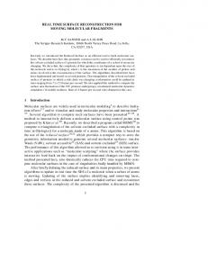
8.2. Density estimation Density estimation 90 is a relatively recent development where particle tracing is used to compute a mesh, which is then fit for display. The algorithm is composed of three phases. First, a particle tracing pass is performed to detect where particles intersect surfaces (figure 16a). These intersections (hit points, see figure 16b) are stored in a list. Second, for each receiving surface an approximate irradiance function H (u; v) is constructed based on these hit points (figure 16c). Finally, this function is further approximated to a more compact form H¯ (u; v) (figure 16d) which is suitable for hardware rendering or ray tracing display.

The number of particles a patch receives determines its radiance. In particle tracing, a very large number of particles have to be traced before a reasonable approximation to the actual solution of the rendering equation is reached. This result is due to the law of the large numbers, which states that the larger the number of samples (traced particles), the better the agreement of the estimator with the actual value.

8.1. Parallel particle tracing First impressions of the particle tracing seem to suggest that it is within the class of embarrassingly parallel problems. The path of each particle may be computed independently of all other particles. If each processor stores the entire scene description in its local memory, then particle tracing is completely parallelisable 112 40 . Each processor will trace a large number of particles independently of the work of other processors. After the computation finishes, the only work that remains is to collate the results of each processor to determine the irradiance of all patches.

a. Particle tracing c. Density estimation

b. Particle hit points d. Meshing

;

If a scene is too large to fit into a single processor’s memory, things become considerably more difficult. Firstly, the data structure that stores where particles have hit surfaces now has to be distributed across a number of processors. Updating this data structure may therefore involve communication between processors, in a similar vain to radiosity updates. Secondly, whereas in ray tracing, certain types of rays exhibit exploitable coherence, the random nature of the Monte Carlo method restricts any similar approach based on the coherence of particle paths. Precomputational analysis using the position and intensity of light sources may provide some indication as to voxels likely to be requested by particle paths leaving the light sources. The subsequent path of the particle is determined by the nature of the environment. To a certain extend these problems can be solved using standard parallel processing techniques such as prefetching and profiling 101 102 . This, however, implies an extra preprocessing step. ;

Figure 16: Density estimation All three steps can be parallelised, with synchronisation only occurring inbetween consecutive steps. The implementation in 112 uses files for communication between steps. The first step is straightforward, as it is assumed that the scene description can be replicated. Each processor creates as output of the first step a file containing the generated hit points. A master processor then takes the hit points generated by all processors and reorders them so that each hit points is matched with its surface. In the second parallel step, the density estimation and meshing is performed. Each processor receives an initial number of surfaces to act upon and when this work is finished, the remainder of the work is distributed on demand. When a surface is completely meshed it is written to file. The algorithm terminates when all processors have finished their work. For relatively small numbers of processors this algorithm performs reasonably well. However, it is assumed that the


environment fits into a single processor’s memory and it therefore precludes the rendering of very complex scenes. It does allow larger scenes to be rendered than radiosity approaches that replicate their data, as it is not the meshing that is replicated, but only the surface geometry. 9. Data distribution and data locality As can be deduced from the above, global illumination algorithms have certain characteristics that make them difficult to parallelise. First, the sheer amount of data often involved in rendering, requires the database to be distributed across the available processors. The complexity of the models to be rendered is increasing all the time, for example due to 3D model grabbing algorithms becoming more widely available. Such algorithms tend to generate huge amounts of polygonal surfaces. Unfortunately, a distributed scene implies that processors either have to migrate tasks, or fetch data. This incurs overheads that prevent algorithms to scale beyond a fairly small number of processors. Second, data access patterns are often unpredictable and changing rapidly, which means that for large scenes caching strategies may be less effective. Third, load patterns may vary significantly, which may render profiling and other cost estimations of less value as they only account for the expected average load. Fourth, near the end of the computation there usually is less unfinished work in the system which makes it difficult to keep all processors busy. The termination phase can therefore take a substantial amount of time, which reduces efficiency and scalability. Keeping processors busy during the last phase of the computation is largely an unsolved problem, since standard task stealing strategies may well introduce a substantial amount of data communication to match the data and the newly stolen tasks. To some extent the above problems may be addressed by localising computations: when it is possible to partition the computations or the data in subtasks in such a way that the interaction with other subtasks is minimal, then data communication may be reduced and cache trashing prevented. We will in the following first discuss data distribution strategies and then return to issues of data locality and cache coherence. 9.1. Data distribution When data has to be distributed, a first issue is how scene data should be divided over the processors. Initial data distributions can have a strong impact on how well the system performs. The more evenly the workload associated with the data is distributed, the less idle time is to be expected. In order to be able to distribute a part of the scene, for instance a cell of an octree spatial subdivision, first the expected cost per voxel should be computed. In a second step, the voxels

can be distributed across the processors, preserving data locality as much as possible, while at the same time attempting to equalise the cost per processor. Some initial research has proved that it is possible to estimate the cost of a single ray traversing an octree structure 80 . The number of intersection tests for each node in the octree is computed by averaging the depth of the leaf cells of the octree and then weighting these depths by the surface area of the cells. For each leaf node, the probability that a ray traversing that voxel intersects one of the objects contained within the voxel, is computed as well. The ray traversal cost is then estimated using the average tree depth and the average blocking factor by summing the probabilities that a ray is blocked in the ith voxel but not in the i , 1 preceeding voxels. Repeating this algorithm for each internal voxel, gives the cost per subtree. Alternatively, the cost per voxel could be predicted by estimating the number of rays that would traverse each voxel during rendering 57 81 . Such an algorithm would take into account the distribution of objects over the scene, as well as the view point and the position of light sources. The data distribution would therefore be tailored to the particular view point chosen. It may therefore well outperform other data distribution algorithms. ;

The second step in such data distribution algorithms would take the cost function per voxel as a basis for distributing the voxels across the processors. Such an algorithm has two conflicting goals for achieving a good data distribution. First of all, no matter how the cost of each voxel is computed, the cost of the voxels assigned to a processor should be roughly the same for each of the processors. During rendering, this should simplify the scheduler’s job, because now the scheduler may assume that if equal numbers of ray tasks are handed to each processor, then the workload of each processor should be roughly the same as well. A better load balance should therefore be obtained. The second goal is to maintain coherence as much as possible. If an octree is arbitrarily split up and distributed over a number of processors, tasks may have to be migrated more than necessary. This is especially true for data parallel ray tasks. It also inhibits the possibility of preferred bias scheduling and if data needs to be fetched, it is likely to involve many different processors. Maintaining coherence on the other hand, solves most of these problems, but unfortunately, requires sometimes the cost function of the voxels to be ignored, leading to a less favourable load balance. Algorithms to distribute octree branches over processors may attempt to split the octree into separate branches as near to the root of the tree as possible. In that case the emphasis is on coherence, so that a ray traversing the octree will not have to be communicated to too many different processors. The cost function assigned to each processor may fluctuate between processors. A slightly better, but also more involved algorithm may be region growing 68 , where neighbouring voxels are assigned to the same processor.


Octrees and grids are regular subdivisions that do not always segment a model in an optimal way. Better data coherence may be obtained with a space partitioning that is aligned with the internal structure of the model. The BSPtree method uses planar surfaces of the model to derive a binary space partition. Several strategies have been developed to choose the most suitable faces as primary dividing planes and to optimize the data coherence within the resulting space partitions (preferably cubic and not long and thin) while keeping the number of splitted surfaces as low as possible 22 62 . Meneveaux 59 applies a clustering algorithm to the surfaces in a scene to align the partitioning even better with the structure of the floor plan. ;

9.2. Visibility preprocessing A very fruitful approach is to partition the scene on basis of intervisibility 100 . Energy transfer can only take place between surfaces that are mutual visible. A visibility preprocessing can be used to create local clusters and to calculate visibility between these clusters. This information can be stored in a visibility graph with the clusters as nodes. The graph can then be segmented in groups to perform for instance the group iterative methods that we already encountered in section 5.3. For the clustering, the importance of the energy transfer between surfaces can be taken into account as well. Two surfaces with a high ’form-factor’ interaction are likely to end up in the same cluster 23 . 9.3. Environment mapping However, even with a suitable data partitioning, interaction between data partitions can not completely be avoided, leading to either data or task communication. Reducing communication by applying local ’place holders’ to represent remote objects and space partitions is a recent development. One of the first applications of this idea are the virtual walls (already mentioned in section 6.1). A similar strategy is applied with environment mapping 4 34 . A data distribution can be created in such a way that each processor stores part of the scene and this geometry is surrounded by an environment map. Instead of fetching data from remote processors, or migrating tasks to other processors, a simple table lookup can be performed to approximate a shading value which would otherwise be very costly to compute 82 . ;

9.4. Geometric simplification Geometric simplification is another successful strategy. The basic idea is that if a complex object or a densely populated part of the scene is at some distance, then without sacrifycing accuracy, the complex geometry can be replaced with a simplified geometry carrying the same energy and having similar reflection and emission properties. In addition, under certain circumstances using simplified geometry may increase the quality of sampling as well 52 .

Figure 17: The plants close-by need to be sampled at full resolution, whereas the plants far away can be sampled at a far lower resolution.

An example where the full resolution of geometry data is not always required is given in figure 17. Assuming that the plants are distributed across a number of processors, the processors responsible for the area where the viewpoint is, may occasionally need to access data that is far away. The plants at the back of the greenhouse could be fetched at a far lower resolution without impacting the quality of the sampling. There are many different ways in which geometry can be simplified or stored at different resolutions. The methods that should be considered are ones where geometry is replaced with simpler geometry (geometric simplification and level of detail techniques), and techniques where geometry is augmented with an extra data structure (impostors, grouping of patches). Geometric simplification algorithms attempt to reduce the polygon count of objects by replacing large groups of small surfaces by a small group of larger surfaces 41 25 . Such algorithms usually do not replace different surface reflectance properties by an average brdf. However, preserving average material properties is important for geometric simplification algorithms to be useful in realistic rendering algorithms. This issue is addressed by Rushmeier et. al. 86 . ;

Levels of detail algorithms build a hierarchy of models in different resolutions by repeatedly applying some geometric simplification algorithm. In parallel rendering, building this data structure would be performed as a pre-processing step. During rendering, the distance between the origin of a ray (whether in ray tracing, particle tracing or radiosity) and the


data requested should be used to determine the level in the hierarchy. The further the distance between two processors, the smaller the amount of data sent.

when enough work is available or when its contribution to the final rendering wins over processing other data voxels.

A locally dense occupation of small polygons, e.g. a plant, can be grouped or clustered and replaced by an enclosing volume that inherits the same reflection, emission, absorption or transparancy properties as the original. Methods may differ in the way they represent these properties, either as transfer functions 52 , volume rendering 91 or blocking and reflection estimation 86 .

10. Discussion

Impostors 24 58 work in much the same way as environment maps, the difference being that rather than replacing the surroundings of an object with a box plus texture map, the object itself is replaced with a simple cube plus texture map. Therefore, impostors borrow from both environment mapping in construction and geometric simplification in usage. ;

9.5. Directional caching The disadvantage with the above techniques is that they all require a pre-processing stage, and sometimes even require user intervention, which makes them slightly awkward to use. A possible method to overcome this, is to build a datastructure on the fly. If a processor holds a part of the scene, then locally sampling proceeds as normal. For rays that leave a processor’s local subspace, this data structure is queried. If there is sufficient information present in the data structure, this is used (as in environment mapping). If not, the ray task is migrated to another processor and when a shading result is returned, it is used for both shading the ray and updating the data structure. The further the computation proceeds, the less communication between processors will be necessary, as processors will build up an image of what surrounds them. We term such methods “directional caching” 26 . 9.6. Re-ordering computations All the above methods try to reduce the amount of data needed from remote processors in order to reduce the communication overhead or to prevent local caches from trashing. In combination with these methods or when the above methods loose their strength then yet another strategy can be applied: re-ordering of the computations to improve cache performance. The general idea is that request for remote data can be surpressed at the cost of storing some extra state information and at a possible penalty for not taken the optimal order of computations. For instance in progressive radiosity some shootings may be deferred which may lead to a slower convergence. This penalty may be accepted as it will lead to a much higher efficiency in the use of remote data citeMene97a. In Pharr et al.71 and Nakamura and Ohno63 rays are processed in voxel order. A voxel with object data is only loaded

Photo-realistic rendering of large models remains still very much an open research issue. Model sizes rapidly increase and models of more than 1 GB of data including radiosity meshes and textures are no exception anymore. Utilizing the computing and memory resources of a distributed set of processors is very attractive in that respect. However, task and data distribution generate their own problems which are not trivial to solve. In this overview we started with load balancing and load scheduling strategies and we ended with data distribution and data locality methods. This order in itself illustrates the shift from simple to more complex and larger models. The larger the models will become, the more emphasis will be put on cache-coherence improving methods. The above discussed methods are only a few of a large number of possible ways to proceed. This state of the art report has also shown that parallel photo-realistic graphics is a challenging area of research which is being actively pursued by a relatively small number of groups. Two significant forums exist specifically for the presentation and discussion of ideas in this area, the Parallel Rendering Symposium and the Eurographics Workshop on Parallel Graphics & Visualisation (http://www.irisa.fr/caps/workshop/). In addition, a number of key journals have published special issues on this topic, for example, Parallel Computing, vol 23, no. 7, July 1997. We believe that parallel photo-realistic graphics will continue to be a vibrant research topic in the future. Acknowledgements All images were rendered using the Radiance lighting simulation package 107 . Thanks to Arjan Kok and Jan Eek for allowing us to use the results of their modelling efforts. This work was partly funded by the EC under TMR grant number ERBFMBICT960655. References 1.

B. Arnaldi, T. Priol, L. Renambot, and X. Pueyo. Visibility masks for solving complex radiosity computations on multiprocessors. Parallel Computing, 23(7):887–897, jul 1997. Special Issue on Parallel Graphics and Visualisation.

2.

B. Arnaldi, X. Pueyo, and J. Vilaplana. On the division of environments by virtual walls for radiosity computation. In Photorealism in Computer Graphics, pages 198–205, 1991. Proceedings 2nd EG Rendering Workshop.


3.

D. Badouel, K. Bouatouch, and T. Priol. Distributed data and control for ray tracing in parallel. IEEE Computer Graphics and Applications, 14(4):69–77, 1994.

4.

J. F. Blinn and M. E. Newell. Texture and reflection in computer generated images. Communications of the ACM, 19(10):542–547, okt 1976.

5.

K. Bouatouch, D. Menard, and T. Priol. Parallel radiosity using a shared virtual memory. In First Bilkent Computer Graphics Conference, ATARV-93, pages 71– 83, Ankara, Turkey, jul 1993.

6.

K. Bouatouch and T. Priol. Parallel space tracing: An experience on an iPSC hypercube. In N. MagnenatThalmann and D. Thalmann, editors, New Trends in Computer Graphics (Proceedings of CG International ’88), pages 170–187, New York, 1988. SpringerVerlag.

7.

K. Bouatouch and T. Priol. Data management scheme for parallel radiosity. Computer-Aided Design, 26(12):876–882, dec 1994.

8.

M. B. Carter and K. A. Teague. The hypercube ray tracer. In D. Walker and Q. Stout, editors, The 5th Distributed Memory Computing Conference Vol. I, pages 212–216. IEEE Computer Society Press, apr 1990.

9.

A. Chalmers and J. Tidmus. Practical Parallel Processing: An Introduction to Problem Solving in Parallel. International Thomson Computer Press, London, 1996. ISBN 1-85032-135-3.

10. A. G. Chalmers. Occam - the language for educating future parallel programmers? Microprocessing and Microprogramming, 24:757–760, 1988. 11. A. G. Chalmers and D. J. Paddon. Parallel processing of progressive refinement radiosity methods. In 2nd EG Workshop on Rendering, pages 1–11, Barcelona, Spain, may 1991. 12. J. G. Cleary, B. M. Wyvill, G. M. Birtwistle, and R. Vatti. Multiprocessor ray tracing. Computer Graphics Forum, 5(1):3–12, mar 1986. 13. M. F. Cohen, S. E. Chen, J. R. Wallace, and D. P. Greenberg. A progressive refinement approach to fast radiosity image generation. In J. Dill, editor, Computer Graphics (SIGGRAPH ’88 Proceedings), volume 22, pages 75–84, aug 1988. 14. M. F. Cohen and D. P. Greenberg. The hemi-cube: A radiosity solution for complex environments. In B. A. Barsky, editor, Computer Graphics (SIGGRAPH ’85 Proceedings), volume 19, pages 31–40, jul 1985. 15. M. F. Cohen and J. R. Wallace. Radiosity and Realistic Image Synthesis. Academic Press, Inc., Cambridge, MA, 1993.

16. M. . der Zwaan, E. Reinhard, and F. W. Jansen. Pyramid clipping for efficient ray traversal. In P. Hanrahan and W. Purgathofer, editors, Rendering Techniques ’95, pages 1–10. Trinity College, Dublin, Springer - Vienna, June 1995. proceedings of the 6th Eurographics Workshop on Rendering. 17. M. A. Z. Dippé and J. Swensen. An adaptive subdivision algorithm and parallel architecture for realistic image synthesis. In H. Christiansen, editor, Computer Graphics (SIGGRAPH ’84 Proceedings), volume 18, pages 149–158, jul 1984. 18. P. Dutré. Mathematical Frameworks and Monte Carlo Algorithms for Global Illumination in Computer Graphics. PhD thesis, Katholieke Universiteit Leuven, Belgium, sept. 1996. 19. M. Feda. Parallel radiosity on transputers with low communication overhead. In S. Ferenczi and P. Kacsuk, editors, Proceedings of the 2nd Austrian-Hungarian Workshop on Transputer Applications, pages 62–70, Budapest, Hungaria, sep–oct 1994. Hungarian Transputer Users Group and Austrian Centre for Parallel Computing. Report KFKI-1995-2/M, N. 20. M. Feda and W. Purgathofer. Progressive refinement radiosity on a transputer network. In 2nd EG Workshop on Rendering, Barcelona, Spain, may 1991. held in Barcelona, Spain; 13-15 May 1991. 21. C.-C. Feng and S.-N. Yang. A parallel hierarchical radiosity algorithm for complex scenes. In 1997 Symposium on Parallel Rendering, pages 71–77. ACM SIGGRAPH, oct 1997. ISBN 1-58113-010-4. 22. H. Fuchs, Z. M. Kedem, and B. F. Naylor. On visible surface generation by a priori tree structures. In ACM Computer Graphics, volume 14, pages 124–133, July 1980. 23. T. A. Funkhouser. Coarse-grained parallelism for hierarchical radiosity using group iterative methods. In H. Rushmeier, editor, SIGGRAPH 96 Conference Proceedings, Annual Conference Series, pages 343–352. ACM SIGGRAPH, Addison Wesley, aug 1996. held in New Orleans, Louisiana, 04-09 August 1996. 24. T. A. Funkhouser and C. H. Séquin. Adaptive display algorithm for interactive frame rates during visualization of complex virtual environments. In J. T. Kajiya, editor, Computer Graphics (SIGGRAPH ’93 Proceedings), volume 27, pages 247–254, aug 1993. 25. M. Garland and P. S. Heckbert. Surface simplification using quadric error metrics. In T. Whitted, editor, SIGGRAPH 97 Conference Proceedings, pages 209–216. ACM SIGGRAPH, Addison Wesley, aug 1997. 26. R. Germs, E. Reinhard, and F. W. Jansen. Directional caching strategies. Submitted for publication, 1998.


27. A. S. Glassner. Space subdivision for fast ray tracing. IEEE Computer Graphics and Applications, 4(10):15– 22, oct 1984.

40. A. Heirich and J. Arvo. Scalable monte carlo image synthesis. Parallel Computing, 23(7):845–859, July 1997.

28. A. S. Glassner, editor. An Introduction to Ray Tracing. Academic Press, San Diego, 1989.

41. H. Hoppe, T. DeRose, T. Duchamp, J. McDonald, and W. Stuetzle. Mesh optimization. In J. T. Kajiya, editor, Computer Graphics (SIGGRAPH ’93 Proceedings), volume 27, pages 19–26, aug 1993.

29. C. M. Goral, K. E. Torrance, D. P. Greenberg, and B. Battaile. Modeling the interaction of light between diffuse surfaces. In Computer Graphics (SIGGRAPH ’84 Proceedings), volume 18, pages 213–222, jul 1984. 30. P. Green and E. Morgan. Parallelisation schemes for the progressive refinement radiosity method for the synthesis of realistic images. In P. Nixon, editor, Transputer and Occam Developments (Proceedings of the 18th World Occam and Transputer User Group Technical Meeting, pages 97–112, Amsterdam, apr 1995. IOS Press. ISBN 90-5199-222-X.

42. S. E. Hyeon-Ju Yoon and J. W. Cho. Image parallel ray tracing using static load balancing and data prefetching. Parallel Computing, 23(7):861–872, jul 1997. Special Issue on Parallel Graphics and Visualisation. 43. V. ˙I sler, C. Aykanat, and B. Özgüç. Subdivision of 3D space based on the graph partitioning for parallel ray tracing. In Proceedings of the Second Eurographics Workshop on Rendering, Barcelona, Spain, may 1991.

31. S. A. Green and D. J. Paddon. Exploiting coherence for multiprocessor ray tracing. IEEE Computer Graphics and Applications, 9(6):12–26, nov 1989.

44. F. W. Jansen and A. Chalmers. Realism in real time? In M. F. Cohen, C. Puech, and F. Sillion, editors, 4th EG Workshop on Rendering, pages 27–46. Eurographics, jun 1993. held in Paris, France, 14–16 June 1993.

32. S. A. Green and D. J. Paddon. A highly flexible multiprocessor solution for ray tracing. Technical Report TR-89-02, Computer Science Department, University of Bristol, Merchant Venturers Building, Woodland Road, Bristol BS8 1UB, mar 1989.

45. J. P. Jessel, M. Paulin, and R. Caubet. An extended radiosity using parallel ray-traced specular transfers. In 2nd Eurographics Workshop on Rendering, pages 1–12, Barcelona, Spain, may 1991. held in Barcelona, Spain; 13-15 May 1991.

33. S. A. Green and D. J. Paddon. A highly flexible multiprocessor solution for ray tracing. The Visual Computer, 6(2):62–73, mar 1990.

46. D. A. J. Jevans. Optimistic multi-processor ray tracing. In R. A. Earnshaw and B. Wyvill, editors, New Advances in Computer Graphics (Proceedings of CG International ’89), pages 507–522, New York, 1989. Springer-Verlag.

34. N. Greene. Environment mapping and other applications of world projections. IEEE Computer Graphics and Applications, pages 21–29, nov 1986. 35. P. Guitton, J. Roman, and C. Schlick. Two parallel approaches for a progressive radiosity. In 2nd EG Workshop on Rendering, pages 1–11, Barcelona, Spain, may 1991. 36. P. Guitton, J. Roman, and G. Subrenat. Implementation results and analysis of a parallel progressive radiosity. In 1995 Parallel Rendering Symposium, pages 31–38. ACM SIGGRAPH, oct 1995. ISBN 0-89791-774-1. 37. P. Hanrahan and D. Saltzman. A rapid hierarchical radiosity algorithm for unoccluded environments. In C. Bouville and K. Bouatouch, editors, Photorealism in Computer Graphics, Eurographics Seminar Series, New York, 1992. Springer Verlag. 38. P. Hanrahan, D. Saltzman, and L. Aupperle. A rapid hierarchical radiosity algorithm. Computer Graphics, 25(4):197–206, aug 1991. 39. P. Hanrahan and D. Salzman. A rapid hierarchical radiosity algorithm for unoccluded environments. Technical Report CS-TR-281-90, Department of Computer Science, Princeton University, aug 1990.

47. J. T. Kajiya. The rendering equation. In D. C. Evans and R. J. Athay, editors, Computer Graphics (SIGGRAPH ’86 Proceedings), volume 20, pages 143–150, aug 1986. held in Dallas, Texas, August 18–22, 1986. 48. M. J. Keates and R. J. Hubbold. Accelerated ray tracing on the KSR1 virtual shared-memory parallel computer. Technical Report UMCS-94-2-2, Department of Computer Science, University of Manchester, Oxford Road, Manchester, UK, feb 1994. 49. H.-J. Kim and C.-M. Kyung. A new parallel ray-tracing system based on object decomposition. The Visual Computer, 12(5):244–253, 1996. ISSN 0178-2789. 50. H. Kobayashi, T. Nakamura, and Y. Shigei. Parallel processing of an object space for image synthesis using ray tracing. The Visual Computer, 3(1):13–22, feb 1987. 51. H. Kobayashi, T. Nakamura, and Y. Shigei. A strategy for mapping parallel ray-tracing into a hypercube multiprocessor system. In N. Magnenat-Thalmann and D. Thalmann, editors, New Trends in Computer Graphics (Proceedings of CG International ’88), pages 160– 169, New York, 1988. Springer-Verlag.


52. A. J. F. Kok. Grouping of patches in progressive radiosity. In M. Cohen, C. Puech, and F. Sillion, editors, Fourth Eurographics Workshop on Rendering, pages 221–231, Paris, France, jun 1993.

64. R. van Liere. Divide and conquer radiosity. In Photorealism in Computer Graphics, pages 191–197, 1991. Proceedings 2nd EG Rendering Workshop.

53. A. J. F. Kok. Ray Tracing and Radiosity Algorithms for Photorealistic Image Synthesis. PhD thesis, Delft University of Technology, The Netherlands, may 1994. Delft University Press, ISBN 90-6275-981-5.

65. I. Notkin and C. Gotsman. Parallel adaptive ray-tracing. In V. Skala, editor, Proceedings of the Third International Conference in Central Europe on Computer Graphics and Visualisation 95, volume 1, pages 218– 226, Plze˘n, Czech Republic, feb 1995. University of West Bohemia. WSCG 95.

54. T. M. Kurç, C. Aykanat, and B. Özgüç. A parallel scaled conjugate-gradient algorithm for the solution phase of gathering radiosity on hypercubes. The Visual Computer, 13(1):1–19, 1997.

66. I. Notkin and C. Gotsman. Parallel progressive raytracing. Computer Graphics Forum, 16(1):43–56, march 1997.

55. Z. Lahjomri and T. Priol. KOAN: A shared virtual memory for the iPSC/2 hypercube. Technical Report Report 597, IRISA, Campus de Beaulieu, 35042 Rennes Cedex, France, jul 1991.

67. D. E. Orcutt. Implementation of ray tracing on the hypercube. In G. Fox, editor, Third Conference on Hypercube Concurrent Computers and Applications, pages 1207–1210, 1988. vol. 2.

56. Lambert. Photometria sive de mensura et gradibus luminis, colorum et umbrae, 1760.

68. T. J. P. Task and Data Management for Parallel Particle Tracing. PhD thesis, University of the West of England, December 1997.

57. J. D. MacDonald and K. S. Booth. Heuristics for ray tracing using space subdivision. The Visual Computer, (6):153–166, 1990.

69. D. Paddon and A. Chalmers. Parallel processing of the radiosity method. Computer-Aided Design, 26(12):917–927, dec 1994. ISSN 0010-4485.

58. P. W. C. Maciel and P. Shirley. Visual navigation of large environments using textured clusters. In P. Hanrahan and J. Winget, editors, 1995 Symposium on Interactive 3D Graphics, pages 95–102. ACM SIGGRAPH, apr 1995. ISBN 0-89791-736-7.

70. S. N. Pattanaik. Computational Methods for Global Illumination and Visualisation of Complex 3D Environments. PhD thesis, National Centre for Software Technology, Bombay, India, feb 1993.

59. D. Meneveaux, E. Maisel, and K. Bouatouch. A new partitioning method for architectural environments. Technical Report TR 3148, INRIA, April 1997. To appear in Journal of Visualization and Computer Animation, 1998. 60. K. Menzel. Parallel rendering techniques for multiprocessor systems. In Proceedings of Spring School on Computer Graphics, pages 91–103. Comenius University Bratislava, jun 1994. Held june 6–9 in Bratislava, Slovakia. 61. S. Michelin, G. Maffeis, D. Arquès, and J. C. Grossetie. Form factor calculation: a new expression with implementations on a parallel t.node computer. Computer Graphics Forum, 12(3):C421–C432, 1993. Eurographics ’93. 62. P. Morer, A. M. García-Alonso, and J. Flaquer. Optmization of a priority list algorithm for 3-D rendering of buildings. Computer Graphics Forum, 14(4):217– 227, October 1995. 63. K. Nakamaru and Y. Ohno. Breadth-first ray tracing utilizing uniform spatial subdivision. IEEE Transactions on Visualization and Computer Graphics, 3(4):316– 328, 1997.

71. M. Pharr, C. Kolb, R. Gershbein, and P. Hanrahan. Rendering complex scenes with memory-coherent ray tracing. In T. Whitted, editor, SIGGRAPH 97 Conference Proceedings, Annual Conference Series, pages 101– 108. ACM SIGGRAPH, Addison Wesley, aug 1997. ISBN 0-89791-896-7. 72. P. Pitot. The voxar project. IEEE Computer Graphics and Applications, 13(1):27–33, jan 1993. 73. M. Potmesil and E. M. Hoffert. The pixel machine: A parallel image computer. In Computer Graphics (SIGGRAPH ’89 Proceedings), volume 23, pages 69–78, jul 1989. 74. T. Priol and K. Bouatouch. Static load balancing for a parallel ray tracing on a MIMD hypercube. The Visual Computer, 5(1/2):109–119, mar 1989. 75. W. Purgathofer and M. Zeiller. Fast radiosity by parallelization. In Proceedings Eurographics Workshop on Photosimulation, Realism and Physics in Computer Graphics, pages 173–183, Rennes, France, jun 1990. 76. R. J. Recker, D. W. George, and D. P. Greenberg. Acceleration techniques for progressive refinement radiosity. In R. Riesenfeld and C. Sequin, editors, Computer Graphics (1990 Symposium on Interactive 3D Graphics), pages 59–66, mar 1990. held in Snowbird, Utah; 25-28 March 1990.


77. E. Reinhard and A. Chalmers. Message handling in parallel radiance. In M. Bubak, J. Dongarra, and J. Wa´sniewski, editors, Proceedings EuroPVM-MPI’97 - Recent Advances in Parallel Virtual Machine and Message Passing Interface (Fourth European PVMMPI Users’ Group Meeting), Lecture Notes in Computer Science (1332), pages 486–493. Springer - Verlag, nov 1997. ISBN 3-540-63697-8. 78. E. Reinhard and F. W. Jansen. Pyramid clipping. Ray Tracing News, volume 8, number 2, may 1995. 79. E. Reinhard and F. W. Jansen. Rendering large scenes using parallel ray tracing. Parallel Computing, 23(7):873–886, July 1997. Special issue on Parallel Graphics and Visualisation. 80. E. Reinhard, A. J. F. Kok, and F. W. Jansen. Cost prediction in ray tracing. In X. Pueyo and P. Schroeder, editors, Rendering Techniques ’96, pages 41–50, Porto, June 1996. Eurographics, Springer Wien. 81. E. Reinhard, A. J. F. Kok, and F. W. Jansen. Cost distribution prediction for parallel ray tracing. Accepted for the Second Eurographics Workshop on Parallel Graphics and Visualisation, 1998. 82. E. Reinhard, L. U. Tijssen, and F. W. Jansen. Environment mapping for efficient sampling of the diffuse interreflection. In G. Sakas, P. Shirley, and S. Müller, editors, Photorealistic Rendering Techniques, pages 410– 422, Darmstadt, jun 1994. Eurographics, Springer Verlag. proceedings of the 5th Eurographics Workshop on Rendering. 83. L. Renambot, B. Arnaldi, T. Priol, and X. Pueyo. Towards efficient parallel radiosity for DSM-based parallel computers using virtual interfaces. Technical Report 3245, Institut National de Recherche en Informatique et en Automatique (INRIA), Campus Universitaire de Beaulieu, 35042 Rennes Cedex, France, sep 1997. 84. L. Renambot, B. Arnaldi, T. Priol, and X. Pueyo. Towards efficient parallel radiosity for DSM-based parallel computers using virtual interfaces. In 1997 Symposium on Parallel Rendering, pages 79–86. ACM SIGGRAPH, oct 1997. ISBN 1-58113-010-4. 85. J. Richard and J. P. Singh. Parallel hierarchical computation of specular radiosity. In 1997 Symposium on Parallel Rendering, pages 59–69. ACM SIGGRAPH, oct 1997. ISBN 1-58113-010-4. 86. H. E. Rushmeier, C. Patterson, and A. Veerasamy. Geometric simplification for indirect illumination calculations. In Proceedings of Graphics Interface ’93, pages 227–236, Toronto, Ontario, may 1993. Canadian Information Processing Society. 87. J. Salmon and J. Goldsmith. A hypercube ray-tracer. In Proceedings of the 3rd Conference on Hypercube

Concurrent Computers and Applications Vol. II, pages 1194–1206. ACM Press, 1988. 88. I. D. Scherson and C. Caspary. Multiprocessing for ray tracing: A hierarchical self-balancing approach. The Visual Computer, 4(4):188–196, 1988. 89. P. Shirley. Physically Based Lighting Calculations for Computer Graphics. PhD thesis, University of Illinois, Urbana-Champaign, nov 1991. 90. P. Shirley, B. Wade, D. Zareski, P. Hubbard, B. Walter, and D. P. Greenberg. Global illumination via density estimation. In Proceedings of the Sixth Eurographics Workshop on Rendering, pages 187–199. SpringerVerlag, June 1995. 91. F. X. Sillion and C. Puech. Radiosity and Global Illumination. Morgan Kaufmann Publishers, Inc., San Francisco, California, 1994. ISBN 1-55860-277-1. 92. J. S. Sing, A. Gupta, and M. Levoy. Parallel visualization algorithms: Performance and architectural implications. IEEE Computer, 27(7):45–55, jul 1994. 93. J. P. Singh, C. Holt, T. Totsuka, A. Gupta, and J. Hennessy. Load balancing and data locality in adaptive hierarchical N-body methods: Barnes-hut, fast multipole and radiosity. Journal of Parallel and Distributed Computing, 27(1):118–141, jun 1995. ISSN 0743-7315. 94. S. Spach and R. Pulleyblank. Parallel raytraced image generation. Hewlett-Packard Journal, 43(3):76–83, jun 1992. 95. W. Stürzlinger, G. Schaufler, and J. Volkert. Load balancing for a parallel radiosity algorithm. In 1995 Parallel Rendering Symposium, pages 39–45. ACM SIGGRAPH, oct 1995. ISBN0-89791-774-1. 96. W. Stürzlinger and C. Wild. Parallel progressive radiosity with parallel visibility calculations. In V. Skala, editor, Winter School of Computer Graphics and CAD Systems, pages 66–74. University of West Bohemia, jan 1994. 97. W. Stürzlinger and C. Wild. Parallel visibility computations for parallel radiosity. In B. Buchberger and J. Volkert, editors, Parallel Processing: CONPAR 94 VAPP VI (Third Joint International Conference on Vector and Parallel Processing), volume 854 of Lecture Notes in Computer Science, pages 405–413, Berlin, sep 1994. Springer-Verlag. ISBN 3-540-58430-7. 98. D. Stuttard, A. Worral, D. Paddon, and C. Willis. A parallel radiosity system for large data sets. In V. Skala, editor, The Third International Conference in Central Europe on Computer Graphics and Visualisation 95, volume 2, pages 421–429, Plze˘n, Czech Republic, feb 1995. University of West Bohemia.


99. I. E. Sutherland, R. F. Sproull, and R. A. Schumacker. A characterization of ten hidden-surface algorithms. Computing Surveys, 6(1):1–55, mar 1974. 100. S. Teller and P. Hanrahan. Global visibility algorithms for illumination computations. In Proceeding SIGGRAPH 93, pages 239–246, 1993. 101. J. P. Tidmus, A. G. Chalmers, and R. M. Miles. Distributed monte carlo techniques for interactive photorealistic image synthesis. In R. Miles and A. Chalmers, editors, 17th World Occam and Transputer Users Group conference, pages 139–147, Bristol, 1994. IOS Press. 102. J. P. Tidmus, R. Miles, and A. Chalmers. Prefetch data management for parallel particle tracing. In A. Bakkers, editor, Parallel Programming and Java, Proceedings of WoTUG-20, volume 50 of Concurrent Systems Engineering, pages 130–137, University of Twente, Netherlands, 1997. World occam and Transputer User Group (WoTUG), IOS Press, Netherlands. 103. I. Verdú, D. Giménez, and J. C. Torres. Ray tracing for natural scenes in parallel processors. In H. Liddell, A. Colbrook, B. Hertzberger, and P. Sloot, editors, Highe-Performance Computing and Networking, volume 1067 of Lecture Notes in Computer Science, pages 297–305. Springer-Verlag, apr 1996. ISBN 3540-61142-8. 104. J. Žára, A. Holeˇcek, and J. Pˇrikryl. Parallelisation of the ray-tracing algorithm. In V. Skala, editor, Winter School of Computer Graphics and CAD Systems 94, volume 1, pages 113–117. University of West Bohemia, jan 1994. WSCG 95. 105. J. Žára, A. Holeˇcek, and J. Pˇrikryl. When the parallel ray-tracer starts to be efficient? In Proceedings of Spring School on Computer Graphics, pages 108–116. Comenius University Bratislava, jun 1994. Held jun 6– 9 Bratislava, Slovakia. 106. J. Wallace, K. Elmquist, and E. Haines. A ray tracing algorithm for progressive radiosity. In Computer Graphics (ACM SIGGRAPH ’89 Proceedings), volume 23, pages 315–324, jul 1989. 107. G. J. Ward. The RADIANCE lighting simulation and rendering system. In A. Glassner, editor, Proceedings of SIGGRAPH ’94 (Orlando, Florida, July 24– 29, 1994), Computer Graphics Proceedings, Annual Conference Series, pages 459–472. ACM SIGGRAPH, ACM Press, July 1994. 108. H. Weghorst, G. Hooper, and D. P. Greenberg. Improved computations methods for ray tracing. Transactions on Graphics, 3(1):52–69, jan 1984. 109. T. Whitted. An improved illumination model for shaded display. Communications of the ACM, 23(6):343–349, jun 1980.

110. H. Xu, Q. Peng, and Y. Liang. Accelerated radiosity method for complex environments. In Eurographics ’89, pages 51–61, Amsterdam, sep 1989. Elsevier Science Publishers. Eurographics ’89. 111. Y. Yu, O. H. Ibarra, and T. Yang. Parallel progressive radiosity with adaptive meshing. In A. Ferreira, J. Rolim, Y. Saad, and T. Yang, editors, Parallel Algorithms for Irregularly Structured Problems (Third International Workshop, IRREGULAR ’96), volume 1117 of Lecture Notes in Computer Science, pages 159–170. Springer-Verlag, aug 1996. ISBN 3-540-61549-0. 112. D. Zareski, B. Wade, P. Hubbard, and P. Shirley. Efficient parallel global illumination using density estimation. In 1995 Parallel Rendering Symposium, pages 47–54. ACM SIGGRAPH, 1995. ISBN 0-89791-7741.