Direct illumination is calculated using shadow photons, as discussed later. ... of specular and glossy objects will spawn lots of recursive calls to the distribution ...
Photorealistic Rendering �� using the PhotonMap Ingo Wald August 1999
Universität Kaiserslautern Fachbereich Informatik AG Numerische Algorithmen Prof. Dr. Stefan Heinrich
Aufgabenstellung und Betreuung: Dr. Alexander Keller
Erklärung Hiermit versichere ich, die vorliegende Arbeit selbständig und nur mit den angegebenen Hilfsmitteln angefertigt zu haben.
Kaiserslautern, den 1. September 1999
III
“Comparisons with existing global illumination techniques indicate that the photon map provides an efficient environment for global illumination” Henrik Wann Jensen “The truth is out there” The X-Files
“Another solution is just to always use enough photons” Henrik Wann Jensen “if it won’t yield to brute force - use a bigger hammer” unknown author
First of all, I wish to thank all those who have contributed to this work, either directly or indirectly: I wish to thank all the members of our group - Alex Keller, Johannes Timmer, Thomas Kollig, Ilja Friedel and Marc Pauly for their help and their company, especially Thomas Kollig, with whom discussions on issues of photorealistic rendering have always been valuable, and who’s advice on Metropolis has been invaluable. I also wish to thank Dr. Alex Keller, for allowing me to do this work, and for helping me in managing it. Finally, I wish to thank Roger Daneker and Rene Schaetzl, for reading and correcting this work, and my girlfriend Gabriele Kaiser, for bearing me when I’ve been stressed, and for cheering me up when I’ve been disappointed.
IV
Contents 1
Introduction
2
The Photon Map 2.1 Basics of Global Illumination . . . . . . . . . . . . . . 2.2 Generating the Photon Map . . . . . . . . . . . . . . . 2.3 The 3d-Tree Photon Map . . . . . . . . . . . . . . . . . 2.3.1 Efficient Construction of Balanced kd-Trees. . . 2.3.2 Efficient Nearest-Neighbour-Query in a kd-Tree 2.4 The GridPhotonMap . . . . . . . . . . . . . . . . . . . 2.5 The Photon Map Shader . . . . . . . . . . . . . . . . .
3
4
1
. . . . . . .
. . . . . . .
. . . . . . .
. . . . . . .
. . . . . . .
. . . . . . .
. . . . . . .
. . . . . . .
. . . . . . .
. . . . . . .
. . . . . . .
. . . . . . .
. . . . . . .
. . . . . . .
. . . . . . .
. . . . . . .
. . . . . . .
. . . . . . .
. . . . . . .
. . . . . . .
3 3 5 7 7 10 11 13
Analysis of the Photon Map 3.1 Efficiency of the Photon Map . . . . . . . . . . . . . . . . . . . . . . . . . . . 3.2 Advantages of the Photon Map . . . . . . . . . . . . . . . . . . . . . . . . . . . 3.3 Disadvantages of the Photon Map . . . . . . . . . . . . . . . . . . . . . . . . . 3.3.1 Dependence on Parameters . . . . . . . . . . . . . . . . . . . . . . . . 3.3.2 Low-Frequency Noise . . . . . . . . . . . . . . . . . . . . . . . . . . . 3.3.3 Blurring . . . . . . . . . . . . . . . . . . . . . . . . . . . . . . . . . . 3.3.4 Energy-Bleeding . . . . . . . . . . . . . . . . . . . . . . . . . . . . . . 3.3.5 Overmodulation . . . . . . . . . . . . . . . . . . . . . . . . . . . . . . 3.3.6 Artifacts Resulting From a Wrong Area Estimate . . . . . . . . . . . . . 3.3.7 Problems arising from the Forward Simulation in Generating the Photons
. . . . . . . . . .
. . . . . . . . . .
. . . . . . . . . .
. . . . . . . . . .
. . . . . . . . . .
. . . . . . . . . .
. . . . . . . . . .
15 15 16 17 18 19 20 23 24 25 27
Photon Map Algorithms 4.1 Testing queried Photons on their Feasibility . . . . . . . . . 4.1.1 Occlusion Testing . . . . . . . . . . . . . . . . . . 4.2 Separate Calculation of Direct Illumination . . . . . . . . . 4.2.1 Monte Carlo Integration . . . . . . . . . . . . . . . 4.2.2 Shadow Photons . . . . . . . . . . . . . . . . . . . 4.2.3 Importance Sampling using Photon Map Information 4.3 Local Pass Integration . . . . . . . . . . . . . . . . . . . . 4.4 Multiple Photon Maps . . . . . . . . . . . . . . . . . . . . 4.5 The Hierarchical Photon Map . . . . . . . . . . . . . . . . . 4.6 Splitting of Caustic Photons . . . . . . . . . . . . . . . . . 4.6.1 Splitting by Brute Force . . . . . . . . . . . . . . . 4.6.2 Splitting Caustic Photons using Metropolis Sampling 4.7 Importance driven Photon Map Generation . . . . . . . . .
. . . . . . . . . . . . .
. . . . . . . . . . . . .
. . . . . . . . . . . . .
. . . . . . . . . . . . .
. . . . . . . . . . . . .
. . . . . . . . . . . . .
. . . . . . . . . . . . .
29 29 30 31 33 34 35 37 39 42 45 45 47 49
V
. . . . . . . . . . .
. . . . . . . . . . . . . .
. . . . . . . . . . . . .
. . . . . . . . . . . . .
. . . . . . . . . . . . .
. . . . . . . . . . . . .
. . . . . . . . . . . . .
. . . . . . . . . . . . .
. . . . . . . . . . . . .
. . . . . . . . . . . . .
. . . . . . . . . . . . .
CONTENTS
VI 4.8
Choosing
Adaptively . . . . . . . . . . . . . . . . . . . . . . . . . . . . . . . . . . . . . .
51
5
Results and Discussion
53
6
Conclusions
63
Chapter 1
Introduction � 1 Recently, the PhotonMap has been introduced into the field of photorealistic rendering in a series of papers ([JC95b], [Jen95], [JC95a], [Jen96a], [Jen96b], [JC98], etc.). Because of its strong impact, the goal of this work was the implementation of the photon map and its integration into an existing rendering platform. While doing this, several problems arose which were first dismissed as implementation problems, but which were soon after revealed to be intrinsic flaws of the photon map method. Since these problems have not yet been sufficiently documented, they have been profoundly investigated in this work. The aim of this work is to analyze and to improve the original method, making it first necessary to name, quantify, classify and document its flaws. We start by briefly summarizing the basics of global illumination in section 2.1, followed by some notes on efficient implementations of the photon map algorithms in sections 2.3.1, 2.3.2 and 2.4. The integration of the photon map into an existing distribution ray tracer is presented in section 2.5, together with a brief summary of how the photon map is used in the original papers. A detailed analysis of the photon map follows in chapter 3, where both its advantages and its disadvantages are discussed. After outlining the problems, several approaches to improve the photon map are proposed and examined in chapter 4. Finally, chapter 5 presents several of the scenes used in our experiments, each with a short discussion of the results when rendering it with the photon map and its different extensions. The conclusions are drawn in chapter 6.
1
���
PhotonMap is a registered trademark of mental ��� images, Gesellschaft f”ur Computerfilm und Maschinenintelligenz mbH & Co KG., D10623 Berlin, Germany. In the sequel, the sign will be omitted.
1
2
CHAPTER 1. INTRODUCTION
Chapter 2
The Photon Map 2.1 Basics of Global Illumination In order to understand the photon map and its problems, we will first discuss some of the basics of photorealistic rendering, by defining the radiance equation: The basic quantity describing the perceivable illumination in a scene is the radiance . For a deeper coverage of the fundamentals of global illumination, together with a complete definition and physical derivation of the term radiance, see [Kel98], [CW93] and [Kaj86]. The radiance equation was first derived in [Kaj86] and is a physically based model for describing the transport of radiance in a scene. Using the notation
�
�
: the surface of the scene, : the hemisphere of all directions
�
at surface position
��� �
,
�� � �� : the radiance leaving ��� � into direction ��� � , ���� � �� : the irradiance at x, i.e. the radiance reaching ��� � from direction ��� � , ���� � �� : the exitant radiance emitted from ��� � into direction ��� � , and ��� � �� �� �� � : the bidirectional scattering distribution function, �� ���� � �� and all radiance incident in � and reflected the radiance � �� is the sum of the emitted radiance into direction � : �� � �� �� ���� � �� �� �! ��� � �� �� �� � ���� � �� � !"$#�%'& ��( � �*) (2.1) � � Let + � �� denote the raycasting function, i.e. ,��-+ � �� is the closest intersection between the surface � of the scene and a ray starting at position ��� with direction � . Then, restricting our problem to vacuum ���� � �� �� �� + � � �� � $.�� , which yields 1 radiation transport , the irradiance can be substituted by �� � �� �� ���� � �� �� !� �� � � �� �� �� � �� + � � �� � � $.�� � !"$#�%'& ��( � �
(2.2)
1 The restriction to vacuum-transport is chosen for reasons of simplicity, since volumetric effects are not covered in this work. For extensions of the PhotonMap to participating media, see [JC98].
3
CHAPTER 2. THE PHOTON MAP
4
The radiance equation is a second kind Fredholm integral equation. With operator, it can be written in operator form as
���
as the kernel of the integral
� �� ������ �)
(2.3)
Inserting equation 2.3 into itself yields
� ��� ������ � �� ������ � �� ������ � �� ������ �*)$)$) � � � � � � �� ��� ��
(2.4) (2.5)
which is called the Neumann-series. A more profound derivation of the Neumann-series can be found in [Kel98], which shows both its correctness and its convergence under certain conditions.
���
�� � ��� � �� �� �� � � ���(!� �� � �� � ( � � �� �
The kernel of the integral operator is the bidirectional scattering distribution function (bsdf), which describes the interaction of light with the surface. The bsdf is defined as
��
�
and describes which fraction of the radiance coming from direction is scattered into direction . The bsdf is a probability density function and can be viewed as describing the probability of a photon with incoming direction to be scattered into direction . Our implementation uses the Ward reflection model [War92], where is modelled to consist of a diffuse, a specular and a glossy part
��
�
���
��� � � ��� � �� ��� � ����� )
���� can be expressed as ���� ���� ��� ��������'���������� (2.6) Diffuse interactions (i.e. applications of �� ��� are called regular, while both specular and glossy interactions are
Using the linearity of the integral operator,
called singular. Slightly glossy interactions may also be approximated by regular interactions, which introduces some small error, but greatly simplifies computations in scenes with lots of slightly glossy objects. As stated above, the bsdf is a probability density function, and even though our implementation only uses the Ward reflection model, the photon map is generally capable of handling any arbitrary pdf. Using 2.6, equation 2.3 can be split into several terms
� ��
� � �� ��� ����� � � �
� �! ������"������$# �) �� is the object’s emittance, given by the material These terms will in the sequel be calculated separately: � % definition, ! ������"������$# describes specular and glossy reflections, and � �� ��� is the diffusely reflected � radiance. can be furtherly split into � � �� ��� � �� ��� ��� �� � � ���� � �� ��� � � �� ��� �� ��� � � �� ��� �! ������"������$# �)
2.2. GENERATING THE PHOTON MAP
�� ��� ��
5
�� ��� �� ���
The first term is called direct illumination, while the second term represents soft indirect describes caustics. Caustics are illumination details created when illumination. The last term light hits a diffuse surface after at least one singular interaction. Using the light path notation, where denotes � denotes a regular ), and a light source, denotes a singular interaction (i.e. an application of �� ����� � Therefore, photons resulting from such interaction, caustics are created by light paths of the form light paths are called caustic photons, all other photons are called diffuse photons. Note that Jensen uses a � � ) (see [JC95b]), which are only a subset of our different definition by considering only direct caustics ( definition.
�
�� ��� �! ������"������ #
�
� �) �! ������"������$#
�
2.2 Generating the Photon Map The photon map is a discrete density approximation ([Kel98]) of the irradiance in the scene. This discrete density is created by using a random walk ([KMS94]), by emitting photons from light sources and tracing them through the scene: Whenever a photon �
interacts with the surface in � , its new position � its incoming direction and its energy are stored in an array called the photon map data structure.
� �
� $
� � � � �� � �
� � + � � � �� �
void PhotonMapShader::RandomWalk() { for each LightSource LS { // calculate ������� ���!#"�nr $ of photons on source LS
�����%'����& ��� �)��( � ������� ���! � ��� *!� �-,���./� . �� { for + 021�354!67398 ��� ���!#"�$ : �;����� ��=� �������@!A . @GF H E 021'=98?8 ; if (interaction is singular) { singular = true; } else { if (singular) 1I=G4!67354 : ) causticMap.AddPhoton( else 1I=G4!67354 : ) diffuseMap.AddPhoton( singular = false; } if break; // particle absorbed... 1�3 (interaction 1'=)J�673 6D=)J == absorbed) J
�
�
: � ELK :
} } } }
6
Interaction(x, ,bsdf) corresponds to an application of M�N!O as in the previous section. It uses the bsdf E * in 1 to calculate the interaction of the incoming photon 021P4!6Q8 with the surface. To prevent an infinite number of interactions of a photon, we use the ’Russian Roulette’ approach as presented in [AK90] 4 to choose whether the photon is absorbed or not. This method is also used to choose the type of interaction (i.e. E *#R E *?S or E *!T ). The out-scattering 6U= and direction is generated according to the chosen interaction type. Interaction returns both the new direction 2 < � " 5 V # W X 9 Y # W X � V ? Z $ E � N =G['\ " N 9our application, � ): Each subtree with its H H
� � � 2 root node in level is partitioned with respect to dimension , such that each node H in the left subtree of
is smaller than , and each node in the right subtree is larger than (with respect to dimension ):
� ��
�
2121
4
,+,+
� � � � � �)E� F��P@ ������ 0 8#4 ������� � B F��P@ ������ 0 8 � � S�� �S�� � S
4343
14
0/0/
13
('(' .-.-
6
*)*)
6565
12
3
����
$#$#
7
����
8
&%&%
10
2
5
1
E8DE8DE8D EDEDED 8ED ED
��
6
9
C8BC8BB8C CBCBBC 8CB CB
1
�
(2.7)
987987789 987987789 987987789 979779 :8:8;8:;8;8:8:8;8:;8;8:8:8;8:;8;8::;:;; A@8A@8@8A A@A@@A ?8>?8>>8Q? =8? =8 N) { minL = l; r = minR; Swap(p,root,l.node); ++l; } else { Swap(l.node, r.node); ++l; ++r; } } BuildTree(p, N, LeftSon(root), level+1); BuildTree(p, N, RightSon(root), level+1); } KD::BuildTree(Photon *p, int N) { BuildTree(p,N,1,0) } class Index { int mask, node, level; Index(int root) { // initialize to root element node = mask = root; level = 0; } void operator++() { // step to next element in subtree node++; if ((node >> level) != mask) { level++; node = mask 0) { // left subtree is 1�closer Query(neighbours, , LeftSon(node), level+1); if (projDist < neighbours.MaxDistance()) { �#H F ��� if ( < neighbours.MaxDistance()) �#H F ��� neighbours.Process(node, ); � 1 Query(neighbours, , RightSon(node), level+1); } } else { // right subtree is closer
�
. . .
} }
�
2.4. THE GRIDPHOTONMAP
11
2.4 The GridPhotonMap Since a large part of the rendering time is spent in the nearest-neighbour-query, an implementation which is faster than the kd-tree would result in a significant speedup. Therefore, additional algorithms have been developed and tested, in which the most promising approach was using a regular grid for storing the photons. The grid needs additional memory for representing the voxels: In our implementation, this is exactly one pointer and one integer (for tagging) per voxel, which is negligible when using a reasonable ratio of photons to voxels (even a ratio such low as 10:1 would yield a memory overhead of less than 5%).
Y�� �� � ��
A grid of resolution
3
can be stored and accessed by
struct Voxel { Photon *photon; int tag; } voxel[ Y K QK ];
��� ��� 4 4 Voxel(� Y �� � ��� ) = voxel[� Y
U
Y 0 �� �
U ������ 8 ] voxel[(k*K+j)*K+i]
voxel[] pointers to cells.
photons in voxel i,j,k
photons
photons in voxel i+1,j,k
photon[]
As compared to a kd-tree, the regular grid is not adaptive, and therefore reaches optimal performance only when photons are well distributed in the scene. While this is often the case for diffuse photons, it may be problematic with caustic photons, which tend to be clustered. Specifying a maximum search-radius yields performance-gains even in this case. Constructing the regular grid is done ’in place’ in a very straightforward way, by using QuickSort’s in the different dimensions and linking pointers into the array. Since the implementation is straightforward, the code is omitted because of its length. Having voxels, the average complexity for building the grid is
�
�
M 0 8 �C � > �
U
> ��
U �
� > �� �
� � 0 �> �
8
Finding the nearest neighbours in the grid is done by processing the 1 voxels in an order similar to a 3-dimensional seed-fill. The seed voxel R!??S is the voxel containing the query-point . The improved performance is due to the fact that the photons in the seed voxel are already very close to the query-point and therefore very likely to be candidates. As a result, the maximum candidate distance diminishes quickly, and results in fast culling, since only voxels closer 1 current F 0!8 have than to be processed.
�
�
�
3 In non-cubical scenes, each dimension of the grid can be subdivided with a different resolution to match the scene’s different extents in different dimensions. S CENE 10, for example, is best voxelized in a resolution of where .
�����������������
�������������������
CHAPTER 2. THE PHOTON MAP
12 Query works as follows:
1�
Query( , neighbours) { currentTag = currentTag+1; // 1�generate a new tag for this query Get Voxel R!??S which contains Clear(neighbours); 1� ProcessVoxel( R!??S , , neighbours) } 1� , neighbours): ProcessVoxel(V, { // first: tag current voxel... V.tag = currentTag; // second: process all photons in current voxel for each photon : ��� 1����� � , PhotonMap �
Color ShadePhotons(Intersection { PhotonList + ; E *?S = intersection.Object.bsdf.E *?S ; p.Clear( );
F � > . 1 map.Query( �9��?*#R!?�2��� & � � Y�X !�� & )
Color PhotonMapShader::Shade(Intersection { F � > , H !E'E PF 9+ , return ShadePhotons( F � > , � PF � 9+ , + ShadePhotons( }
� ��� � � � � ��� � � �
9+
�
SG� N)N � R! ) �!� � R2���/� );
In calculating ] * , the photon map shader may also incorporate such extensions as the separate calculation of direct light or the local pass. These extensions, however, will themselves use the above methods for calculating the estimate. In [Jen96a], Jensen utilizes the photon map to get a coarse approximation of global illumination. Based on the influence of the sample on the image, heuristics are used to decide whether the estimate from the photon map is used or whether a more complex computation is done. If the contribution of the sample is small, i.e. because it is only a single sample ray in the local pass or because it is attenuated by a small brdf, then the photon map approximation is used directly. Otherwise, if the ray is a primary ray or the point was reached by several perfect reflections, the point is considered important, and the shading is done by more accurate Monte Carlo integration, which in fact is a local pass. This notably improves image quality, but is very time-consuming and can only be applied under certain conditions. Jensen applies Ward’s irradiance caching ([WH92]) on lambertian surfaces which achieves faster rendering times by interpolation. Because of the fact that the radiance estimate is only used as an approximation in more correct Monte Carlo integration, its quality is far less important. In this case ’blurring can even be seen as an advantage’ ([Jen96a]) for reducing noise. Artifacts in the estimate are partly smoothed away by the local pass and partly dominated by direct light. However, a closer look often reveals remains of these artifacts, mainly noise and blurring, especially in caustics, where the radiance estimate has to be visualized directly. Artifacts like energy-bleeding or overmodulation did not appear in the original papers because of suitably modelled scenes. Direct illumination is calculated using shadow photons, as discussed later. This, however, is also only applicable under certain conditions. Caustics are treated separately: They are rendered directly by the photon map. Jensen admits that parameters have to be adjustet to find a tradeoff beween blurred caustic borders and noise in the caustics (see [Jen96b]: “If the parameters are badly chosen, the caustic will either become too blurred or too noisy”). To improve caustics, many more photons are used to represent caustics than are used for diffuse illumination. Jensen uses projection maps ([JC95b]) to increase the number of caustic photons by emitting photons directly from the light sources towards specular objects. This method is only capable of producing direct caustics, but performs well under this limitation.
Chapter 3
Analysis of the Photon Map 3.1 Efficiency of the Photon Map The efficiency of the photon map is believed to depend only on the efficiency of the radiance estimate, which mainly depends on the number of photons used, and which is otherwise independent of scene complexity and geometry. This is proposed as one of the main features of the photon map, making it seemingly possible to render highly complex scenes at moderate cost. However, though it is true that the largest portion of the rendering time is spent in the radiance estimate (querying and shading of the photons), the overall time spent on the estimates is the product of the time spent per estimate and the number of estimates evaluated. Therefore, the “efficiency of the photon map” depends on both the efficiency of the estimate and on the efficiency of the rest of the renderer in keeping the number of estimates small. Therefore, the overall rendering time depends on 3 factors: efficiency of the distribution ray tracer in keeping the number of shader calls small efficiency of the shader in keeping the number of estimates small efficiency of the estimate. The argument of efficiency beeing independent from scene complexity only applies to the last item. The efficiency of the distribution ray tracer into which the photon map shader is built (see section 2.5) has great influence on rendering time: If the scene is highly complex, rendering time will increase because of more expensive ray intersections. Additionally, lots of specular and glossy objects will spawn lots of recursive calls to the distribution ray tracer, manifolding the number of shader calls independently from the photon map. The second factor is the time spent in the photon map shader: Using a local pass manifolds the number of estimates. Independent calculation of direct light may also increase rendering cost under certain circumstances, mainly when having many light sources. These two items imply that realistic scenes - which are highly complex scenes with several light sources and lots of specular and glossy objects - will require high rendering times independently from the number of photons used (see discussion on MM ACK in chapter 5). Rendering cost for the photon map estimate also consists of a preprocessing part (RandomWalk and BuildTree), which can be considered to be constant, since it is not affected by the number and complexity of shader-calls. Preprocessing cost is generally small compared to rendering time: Each photon requires exactly one ray intersection in the random walk step, whereas the distribution ray tracer generates 4 million rays alone for the primary rays in a PAL-resolution image with an oversampling rate of 8 sample per pixel. However, several of the later proposed algorithms will require higher preprocessing times. When using a kd-tree or a regular grid, the time for building the acceleration structure is negligible.
15
CHAPTER 3. ANALYSIS OF THE PHOTON MAP
16
The cost of the radiance estimate is small even with moderately sized photon maps (up 1 to about 250.000 photons). The dominating cost in the estimate is the cost for finding the nearest neighbours to . As Jensen correcly states, increasing the number of overall photons (while keeping fixed) increases rendering cost but slightly. This is verified in the following table, and is due to the that the cost for the query is closely related to the depth of the tree (which > 0 fact � ,�� 4 � ,�� 8 =391s and M 0 � , 4 � ,�� 8 =614s, where 10-folding is , ): Take, for example M the number of photons results in a mere 55% increase in rendering time. (Note that for each parameter pair in the table, exactly the same number of rays are shot).
U V � � X Y
X
X
X
(in sec) N=100k N=1M
k=10 72 156
k=100 391 614
k=1000 1823 4413
X
Contrary to this, Jensen’s conclusion that the resolution of the photon map could be increased without notable increase in rendering time could not be completely verified, since increasing requires increasing by the same factor to yield the same image, since changing the ratio affects the final image (see figure 3.1 in section 3.3.1). Therefore, rendering cost will very well increase when using more photons, since influence of on 8 M � R2��� � �G�� is at least linear. In the above 0 4 8 0 4 � � , � � � , � � , � ,��� =4413s. When using a local pass, can example M =391s would become M be kept small when increasing , since changing the ratio will then not change the final image as visibly; so Jensen is partially correct in this case.
X
X �
X
X X �
3.2 Advantages of the Photon Map The photon map has several advantages over many other illumination algorithms. Since most of these advantages are already sufficiently published in the original papers, they are only briefly summarized here: High quality: Incorporates almost any illumination features, including caustics and volumetric effects Flexibility: Allows for the use of arbitrary object types and arbitrary bsdfs Adaptive to local illumination density Efficiency (of the estimate) is independent of scene geometry Simplicity of code Easily understandable The photon map - as proposed in the original papers - is generally able to render high-quality images of highly complex scenes while using only a moderate amount of resources. The photon map is even able to produce complex illumination features like caustics in a realistically looking way which are otherwise very expensive to compute. The high quality of the rendered images mainly results from the fact that the photon map is able to produce almost any illumination feature: Some features are due to the distribution ray tracer, which creates effects resulting from specular or glossy reflections. Note that lens effects such as motion blur or depth-of-field are also due to the distribution ray tracer. Diffuse illumination and caustics are rendered by the photon map shader. The photon map is also capable of rendering volumetric effects such as fog or volume caustics (see [JC98]), which are not covered in this work. One of the main advantages over other rendering algorithms is that the photon map is able to handle arbitrary illumination models as well as arbitrary object types - objects even don’t have to be parameterizable. This allows even for such complex representations as recursively, fractally, implicitly or procedurally defined objects. Additionally, the photon map does not require the scene to be tesselated (as opposed to finite element methods, mainly Radiosity methods), which enables the photon map to render complex scenes with very compact scene representations. The photon map is also generally capable of using arbitrary bsdfs, which was not tested in our implementation. As compared to finite element methods, the discrete density automatically adapts to local changes in the illumination density. This eliminates the problem of finding a suitable tesselation, which has always been a major problem for these methods. This is especially useful for representing caustics, which have high locality. Another advantage of the photon map is that the time spent in the estimate is independent from scene complexity: With the same number of photons, increasing scene complexity will only increase the time spent for ray-scene-intersections, while most of the time is spent in nearest-neighbour-queries and the radiance estimate, which are not influenced by scene
3.3. DISADVANTAGES OF THE PHOTON MAP
17
complexity. Note that in reality, however, increasing scene complexity would require more photons to be used to achieve comparable quality, and would also increase rendering time due to the distribution ray tracer, as documented in section 3.1. Therefore, this advantage could not be fully verified. The simplicity of the photon map allows for a quick implementation. After the rather technical implementation of the data structures and query-algorithms, the code for the random walk and the estimate is easily created. Since distribution ray tracers are already commonly used, this part is often given in advance. This allows for the photon map to be easily integrated into any existing distribution ray tracer. Flexibility and simplicity of the photon map code also allow to use photon map algorithms and data structures in secondary applications, for example for the efficient sampling of direct light (section 4.2.3) or for getting an estimate for the importance in a scene (section 4.7).
3.3 Disadvantages of the Photon Map While there are already several publications about the photon map in general, none of these sufficiently analyzes the flaws of the photon map method. Therefore, we will first give a detailed description of these problems, which consist of two classes: While the photon map’s artifacts - which are investigated later on in this chapter - are most visibly to the viewer, the photon map also has several intrinsic problems: One of these is that the photon map highly depends on the parameters for the estimate (see section 3.3.1). Secondly, the forward simulation used in the random walk is problematic under certain circumstances, which is covered in section 3.3.7. Some of the already commonly applied extensions like direct light or local pass are also only applicable in suitable settings, see the discussion in the respective sections 4.2 and 4.3. Finally, the efficieny of the photon map highly depends on the efficiency of the distribution ray tracer, as already sufficiently discussed in section 3.1. These problems may result in very poor performance in more realistic scenes.
CHAPTER 3. ANALYSIS OF THE PHOTON MAP
18
3.3.1 Dependence on Parameters
X
X
The quality of the estimate highly depends on the parameters, mainly the number of overall photons and the number of queried neighbours . While it is clear that increasing affects the quality of the estimate, the influence of is less obvious. The critical parameter was found to be the ratio of : Using smaller values for will require fewer neighbours to be queried, resulting in a smaller query-ball and increasing low-frequency noise in the image. On the other side, increasing produces large query-balls, taking photons from a larger volume into account and therefore results in increased blurring. So, the choice is either blurring or noise (see image 3.1).
=50k
X �
=100k
=500k
� � �����������
� � ��� �����
� ��������� � Figure 3.1: Sample images with different parameters decreasing ratio.
X �
and . Note the increased blurring of the shadows with
�
�
The ’optimal’ ratio depends on the scene to be rendered. While ,��. �� ��. �� , was found to be a reasonable value in most of our expirements, this value is subject to change with several other scenes: In the I NVISIBLE DATE scene (see chapter 5), only a small fraction of the photons reaches the room to be rendered. Using the same ratio as in S CENE 6 would result in a huge query-ball in the rendered room. The ratio is less critical when using a local pass, since both blurring and low-frequency noise are reduced by the local pass. Even then, smaller ’s will increase Monte Carlo noise in the local pass, requiring more sample rays to be evaluated.
X �
3.3. DISADVANTAGES OF THE PHOTON MAP
19
Larger values will increase other artifacts like energy-bleeding, visible bands at geometry borders or overmodulation (see later in this chapter). These artifacts will negatively affect the quality of the local pass. The tradeoff between noise and blurring always applies to caustics, where no local pass can be applied (see [Jen96b], ’if the parameters are badly chosen, the caustic will either become too blurred or too noisy’).
3.3.2 Low-Frequency Noise Low-frequency noise is the first-encountered and probably most perceivable artifact of the photon map. It appears when using too coarse a resolution of the photon map and too small a for the estimate (see previous section). When using other ray-based rendering algorithms (raytracing, BDPT, metropolis, . . . ), variance can be reduced by using more samples per pixel, which have to be independent of each other. This independence of samples is no longer assured when using the photon map: Similar rays result in hitting the scene in similar positions, yielding queries at similar positions. Because of the static nature of the photon map - once the discrete density is created, it will never change queries in similar positions will produce very similar - if not the same - neighbour sets 1 . Therefore, the radiance estimate varies but slowly, leading to the low frequency of the noise. To get independent samples, each query should result in a new candidate set. This cannot be realized because of the limited amount of memory: Rendering a PAL-resolution image - about 800 by 600 pixels - with 10 samples per pixel, �� ,� or about five million primary rays. Using a fixed � ,�� and assuming the photons to be one gets � optimally placed, one would need at least �� million photons to assure independent samples for the primary rays alone. 500 million photons would need about 10 Gigabyte of memory and huge rendering times. In fact, the number of photons needed would even be much higher.
����
�
Since lower frequencies are easier perceivable to the eye than higher frequencies, this kind of noise is especially perceivable. Increasing decreases the frequency of the noise, blurring it, but not removing it. The noise in the estimate can also be reduced by increasing the photon density, which will also increase rendering time and memory requirements (see section 3.1). Using a local pass completelys remove low-frequency noise from diffuse illumination, but also increases 1
In fact, the volume of the scene could be tesselated into finitely many voxels in which each point has the same neighbours.
CHAPTER 3. ANALYSIS OF THE PHOTON MAP
20
rendering time and is applicable only in certain settings. Noise can also be reduced by averaging samples from multiple independent maps, see section 4.4. � It can be shown that low frequency noise is not 4 affected by the uniformity of the distribution of the photons. To � , � plane, and calculated the radiance estimate on this plane. All demonstrate this, we created photons directly on a photons have equal energy and direction, their location was chosed according to several sampling patterns, from purely random to patterns with increased uniformity, including jittered, n-rooks-sampling and the halton sequence. One of these patterns is depicted in the left image of the following figure. The right image shows the ’rendered’ image and demonstrates the noise created by the estimate. The dark bands around the border of the image are due to a wrong area estimate as discussed later. Note that this setting is closely related to the table top in S CENE 6.
position of photons
visualized radiance estimate
3.3.3 Blurring Blurring results from the fact that an entire volume - the volume of the query ball - is used for the radiance estimate of a single point. Therefore, the higher the number of photons for the estimate, the larger the query ball and the higher the blurring effect. In consequence, blurring can be decreased by using less photons for the estimate, which in turn increases noise in the image. In [Jen96a], Jensen states that ’the blur in the photon map is actually an advantage since it reduces noise in the final gathering step...’. However, increased blurring not only requires higher rendering-times (because of increased , see section 3.1), it also blurrs correct discontinuities like sharp caustics or shadow borders. Therefore, blurring can hardly be stated as an advantage. As it was done in the previous section, blurring can also be demonstrated by visualizing the radiance estimate of an explicitly generated pattern. This time, the photons are not located in the unit square, but on a simple polygon:
position of photons
radiance estimate (large k)
radiance estimate (small k)
The left image shows the positions of the photons, from which the original figure can be easily recognized. The center image demonstrates several artifacts when using a large number of photons for the estimate: Parts of the figure disappear
3.3. DISADVANTAGES OF THE PHOTON MAP
21
because of an extremely overestimated area (see section 3.3.6). Additionally, the upper ’shadow’ is extremely blurred. The image on the right shows how blurring and dark bands can be diminished by querying fewer photons, which also increases noise.
Loss of Sharp Shadows The most perceivable effect of blurring is the loss of sharp shadows, since the radiance estimate is unable to produce sharp shadow borders: Querying photons in a shadowed area grows the query-ball until it contains photons, however far away and however reasonable these may be (also see energy-bleeding, section 3.3.4). The energy of these photons across the shadow border is therefore blurred into the shadowed area, resulting in a soft falloff of energy instead of a sharp shadow border (see sketch in figure 3.2, effects in figure 3.3).
�� �� �� �� �� � � �� �� ��� �� ��� ��� ��� �� ��� �� ��� �� ��� ��� ��� � ��� � ��� �� �� ��� ������ ��� ��� ��� ��� ��� ��� ��� ��� ��� ��� ��
blocked photons
real shadow border
Shadow-casting object
������ ���� ��� ���� ��������� ������������ �� � � � � � � � � � � � � ������������ �� ��������������������������������������������������������������������� ������������ �� ������������ �� query-position (in shadow)
shadowed area
side view
����
�� ��
����
photons
��
����
�� �� �� ���
query-position (in shadow)
illuminated area
top view
estimated radiance
Figure 3.2: Blurring of shadow borders: The query ball is extended until it contains the required number of photons, even if the query-position is in complete shadow. In the extreme, this leads to a complete removal of some shadows: If the shadow-casting object is relatively small or narrow, i.e. the leg of a table or the thin lamp in I NVISIBLE DATE, the shadow completely disappears when using large ’s for the estimate (see figure 3.3). For the later discussion in section 4.2, shadows have to be classified into 2 kinds: direct shadows and indirect shadows. Direct shadows are shadows resulting from direct illumination. In many scenes, these are the dominating shadows, and can often be rendered efficiently by separate calculation of direct light. Indirect shadows are shadows resulting from indirect light. Since indirect illumination is generally less directional than direct illumination, indirect shadows will appear only in special cases, for example shadows in a caustic or when having a scene illuminated only indirectly by a small, highly energetic area like the slit created by the opened door in the I NVISIBLE DATE scene. Then, this area behaves almost like a light source (see [CRMT91]), casting indirect shadows. Indirect shadows can not be handled by separate calculation of direct light.
22
CHAPTER 3. ANALYSIS OF THE PHOTON MAP
Blurred Caustics Borders For caustic borders, the same argumentation holds as for shadow borders. Queries close to a caustic will extend the ball into the caustic, blurring the caustic border. Blurring of caustics is generally harder to handle than shadows: Since caustics do not result from direct light, they cannot be improved by separate calculation of direct light. Neither can they be handled by a local pass. Quality of caustics can only be improved by using more caustic photons, see section 4.6.
Figure 3.3: Loss of shadows: Shadows under the table and on the chairs in S CENE 6 are completely smoothed away. For a description of the depicted scenes, and some more correctly rendered images, see chapter 5. The lower image shows I NIVISIBLE DATE . Here too, shadows from table, sofa and lamps (as can be seen in a Metropolis-rendered master image in section 5) are missing completely. These shadows are indirect, and can not be rendered by separate calculation of direct light.
Other Effects of Blurring Blurring may also appear in other forms, i.e. by blurring the color. This did not appear in our scenes, but could be seen in several other papers, even in very simple settings. Energy bleeding is also closely related to blurring.
3.3. DISADVANTAGES OF THE PHOTON MAP
23
3.3.4 Energy-Bleeding Energy-bleeding is an effect where energy contributes to the illumination of a location from which it is physically blocked by geometry. It is a consequence of 1 not regarding any geometric or topologic relations in the estimate: A query at position 1 returns the closest photons to without knowing whether these photons really ’belong’ to the query position in a physical sense or not (e.g. whether they are blocked by a wall as sketched in figure 3.4). This effect can be reduced by better plausibility tests, which will, however, introduce new problems (see discussion in section 4.1). Energy-bleeding is closely related to blurring, with the only difference that it is usually much stronger, and that energy will even be ’blurred’ through blocking geometry, making it much more perceivable than ’normal’ blurring, especially in the local pass.
wall
���� ���� �� ���� �� �� ���� �� � � � � � � � � � � � � � � � �� ���� �� �� ���� ����������������������� ������������ �� ������������ �������������������� ��� ������ �� � � �� ���� ���� �� �� ���� ���� �� �� ���� ���� �� �� ���� ���� �� �� ���� ������ invalid photons
eye ray to be shaded
table
correct photons
X
invalid photons on hidden side
query-point
chair
query-point photons on correct side
query-ball
energy bleeding through a wall
energy bleeding through a table
Figure 3.4: Energy bleeding: A query on a wall which is highly illuminated from the hidden side.
Figure 3.5: Effects of energy bleeding: Energy from the backside of the wall bleeds through around the edges of the wall (left side, smoothed by the skipping method). This artifacts even persists when using a local pass, as demonstrated on the right. Energy-bleeding is also responsible for the excessive amount of noise in the local pass, even after over 6 hours of rendering time.
24
CHAPTER 3. ANALYSIS OF THE PHOTON MAP
In the I NVISIBLE DATE scene, for example, energy bleeding produces an entirely highlit wall, if no steps are taken to prevent this. When testing surface normal and photon direction, this effect still appear at the edges of the wall, when photons on the floor and ceiling are found (see figure 3.5). Energy-bleeding is still problematic even using a local pass, as can be seen in the right image. Energy-bleeding also appears in smaller scale, for example even in such an simple setting as S CENE 6: When determining the radiance estimate on the chairs with a large , the query-ball grows until it contains some of the photons from the top of the desk. Then, energy from the top of the table bleeds through to the chairs, as sketched in figure 3.4. A method was implemented which removes energy bleeding (see section 4.1.1); its cost, however, is extremely high, and can only be justified for such severe cases as I NVISIBLE DATE.
H P� F Overmodulation is an artifact which appears as an overly illuminated area. It is due to the fact that the division by �� �
3.3.5 Overmodulation
�
results in a large radiance estimate when radius gets small. This often happens in areas where large clusters of photons are stored, e.g. because of geometry which is close to light sources, like the polygonal ’exit’ letters on the exit sign in figure 3.6. Instead of limiting overmodulation to the lightsources, the blurring effect extends such overmodulated parts of the scene over larger areas.
Figure 3.6: Effects of overmodulation. The high photon density at the light source leads to an entirely overmodulated area. In the lower image depicts the area as it looks when overmodulation is removed by a local pass.
3.3. DISADVANTAGES OF THE PHOTON MAP
25
3.3.6 Artifacts Resulting From a Wrong Area Estimate Artifacts in the estimate sometimes appear as highlighted or darkened bands at geometry borders and edges, i.e. at around the borders of the table top or in the edges of the room, as can be seen in figure 3.8. These artifacts are due to a wrongly � surface estimated area: Since the radiance estimate is in fact a density estimation problem, an estimate for the enclosed area is needed. This is approximated as the area of the query-ball projected onto a plane and is therefore � , resulting in the previously used radiance estimate of � * � . S CENE 6 is an especially good example for the influence of the area estimate: Here, the random walk results in all photons having about the same energy, and the change in the radiance estimate results solely from the change of query ball’s radius. Because of this strong influence of the area estimate, a wrong area estimate implies a faulty radiance estimate.
��
area estimate correct
covered area is larger than esimate area covered by the sphere is a circle estimate is correct
covered area is still too large
area estimate correct again
the same effect when approaching a corner (side view) estimated area (full circle) is larger than the area actually covered radiance estimate Figure 3.7: Wrong estimation of covered area at geometry borders and edges.
CHAPTER 3. ANALYSIS OF THE PHOTON MAP
26
The area estimate is correct whereever the sphere fully covers a flat surface area, but will highly overestimate the area (and therefore underestimate radiance) at geometry borders, where the area actually covered is only a fraction of a circle (see sketch in figure 3.7). This results in a visible falloff of energy near �geometry borders, as can be seen in figure 3.8. The opposite case happens if the sphere covers a surface larger than � , i.e. if the sphere covers both the floor and a table leg, or both a side wall and the floor (also sketched in figure 3.7).
��
S CENE 6
enlarged table borders
enlarged room edges Figure 3.8: Visible bands at geometry borders and edges. The reasons for both artifacts are sketched in figure 3.7. In fact, the same argumentation applies to any non-flat area: In [JC98], Jensen refers to this as “The ... estimate is valid as long as the surface is locally flat”. Since the query-ball is not infinitesimally small, the area in the query-ball very often is not flat, especially in areas with highly complex geometry such as fractally or procedurally defined objects, which are proposed as one of the main features of the photon map. Note that the width of the bands is equal to the radius of the sphere, and can therefore be diminished by using a smaller value if the increased noise can be tolerated.
3.3. DISADVANTAGES OF THE PHOTON MAP
27
3.3.7 Problems arising from the Forward Simulation in Generating the Photons In the original papers, the photons are generated by random walk as shown in section 2.2. This kind of random walk is a pure forward simulation, generating the photons without taking the different importance 2 in different areas into account. In the I NIVISIBLE DATE scene (see chapter 5), this leads to a large number of photons in the room with the lightsource (several thousand photons in the lower example), while only a small fraction of the photons (in our example, less than 50) will actually reach the room to be rendered. This means that the majority of the photons is used to approximate the radiance in the ’unimportant’ neighbouring room, at very high density, while the photon density in the really important room is very low. This implies that a huge number of photons has to be used to get a reasonably high photon density in the interesting areas (see the following figure). The same applies to S CENE 10: Here, the photons are created with equal density in all of the 100 rooms, while only a small fraction of these photons is actually used in the rendering stage. The problem can be solved by using importance driven methods for generating the photons, see section 4.7 photons
importance
S CENE 10
I NVISIBLE DATE
��
The figure depicts the unsuitable distribution of photons that arises when doing a pure forward simulation without ,� equal, interconnected rooms, each with a light taking importance into account. S CENE 10 consists of an array of ,� source. Here, all rooms are approximated with equal density, while samples from only few rooms are actually used in the rendering stage. The left image shows the locations of the photon - as seen from the top - while the right image depicts the importance in this scene. In I NVISIBLE DATE , photon density is almost inversely related to the importance: The right room with the light source is approximated at very high density, while the left room with the viewer receives only a very small fraction of the photons.
2
We will restrict ourselves to an intuitive definition of the term importance. A more profound definition can be found in [PP98].
28
CHAPTER 3. ANALYSIS OF THE PHOTON MAP
Chapter 4
Photon Map Algorithms One method of using the photon map is using it in a standalone version, by directly visualizing the radiance estimate. As stated in the previous chapter, this generates several artifacts, or otherwise requires huge photon map resolutions. Therefore, extensions of the photon map are needed in order to improve the quality of the image. One straightforward way for improving the standalone photon map is the separate calculation of direct light, which often makes up for more than 50 percent of the illumination in simple settings. Several algorithms for the separate calculation of direct light are covered in section 4.2. An also commonly used ’improvement’ is the local pass, which is discussed in section 4.3. Even for these well-known methods - direct light and local pass - a thorough investigation is undertaken, showing both their strengths and their weaknesses. This chapter also provides some additional extensions, which are not yet publicly applied and which aim at removing the problems discussed in the previous chapter.
4.1 Testing queried Photons on their Feasibility As 1�stated in the previous chapter, several of the artifacts result from simply querying and shading the nearest photons to , even if these photons are not reasonable. Since the photon map does not contain any geometric or topologic information, the feasibility of a photon can not be evaluated with absolute certainty. This leaves only some heuristic plausibility tests to prevent shading of unreasonable photons. These tests can be incorporated into either the query or in the shading step. In the first case, photons are stored only if they are presumed feasible. The second solution is to first do a query for all k-nearest neighbours, and then filtering out only the feasible ones before shading. The first method always returns reasonable photons, while the second method may - in the extreme - discard many, if not all, of the found photons. On the other hand, the second method will perform exactly plausiblity tests, which are much less than in the first method, where any visited photon has to be tested. Therefore, the second method is the method of choice if very expensive tests such as occlusion-testing 4.1.1 have to be performed. Less time-consuming tests should be applied directly in the query step. Such tests, however, have to be used very carefully. They often appear plausible, but still remain only heuristics: Most of such tests are reasonable in the general case, but may utterly fail in other environments (see figures 4.2 and 4.1).
��������� ������ ��������������� incoming ����������� ����� � � � � � � � � � ��������������� ������������ ray ����� ����� � � � �
� � � � � � �
� � � � � � �
� � � � � � �
� � � ��������������� ����������������$% ��������&' ������ ������ ����() ����* ������������������ ��������������� %$%$$% '&'&&' )()(() *** a.)
b.)
incoming
ray ��� ��� ��� ��� ��� ��� ��� ��� ��� �� �� �� �� �� �� �� �� �� ������ � � � � � � � � � ��� � � � � � � � � � � �� � � � � � � � � � � � � � � � � � � � � � � � � � � � � � � � � � � � � � � ��� ��� ��� ��� �� �� ������ �� ������ ������ �� ������ ������ ��� ��� ��� ��� ��� ��� ��� ��� ��� �� �� �� �� �� �� �� �� ������ ��� � � � � � � � � � � � � � � � � ��� � � � � � � � � � � � � � � � � � � � � � � � � � � � � � � � � � � � � � � ����� ����� � ������ � ��� � �� � �� � �� � �� � �� � �� � ���� �� � �� �� ��� ��� ��� ��� ��� ��� ��� ��� ��� ��� � �� � �� � ���� ���� � �� �� � �� � �� �� � �� �� � !! ����� � �� � �� � �� ����� �� � �� � �� � �� "##"" �� #"# !! �� ���� Figure 4.1: A simple plausibility test: Testing the angle � + � � � � �-, ��/.10 32
to be below 90 degrees is simple
and seems promising in case a. However, it would be a bad classification in case b. Similar cases can be constructed for other tests. 29
CHAPTER 4. PHOTON MAP ALGORITHMS
30
a.)
incoming ray n(x)
b.)
���� � �
� �����photons �� ������� � � ���
��� ��� ��� ��� ��� � � � ��� ��� ��� ��������������� ��� ������ �� ��� ������� ���� ��� ��� ���� ��� ��� ��� ��� ��� ��� ��� �� ���� ���� ����
valid photons invalid photons
��
incoming ray
n(x)
��
�� �� �� ������������� ����������� �� � � � � � � � � ����������� �� � � � � � � � � �� �� �� �� �� �� �� ����������� �� � � � � � � � � � � � � � � � � � � � � ����������� �� � � � � � � � � � � � � � � � � � � � � �� ����������� �� � � � � � � � � � � � � � � � � � � � � ����������� �� � � � � � � � � � � � � � � � � � � � � ��� ����������� �� � � � � � � � � � � � � � � � � � � � � ����������� �� � � � � � � � � � � � � � � � � � � � � � ������������ �� �� �� �� �� �� �� �� �� �� �� ����������� �� � � � � � � � � � � � � � � � � � � � � ����������� �� � � � � � � � � � � � � � � � � � � � � ����������� ������������������������
valid photons invalid photons
Figure 4.2: Specifying a culling plane by query position and surface normal (dashed line) yields anotherds another plausibility test. Considering photons ’behind’ this culling plane invalid, illumination from the backside (as demonstrated in section 3.3.4) can be prevented on flat surfaces (as sketched in case a), but may be fatal on curved surfaces like in case b, where almost all photons on the ellipsoid are considered invalid. In our implementation, only photons with a ’suitable’ angle between photon direction and surface normal are considered feasible to reduce illumination from the backside. In I NVISIBLE DATE, this test prevents photons from the opposite side of the wall from beeing found, but still results in finding photons on floor and ceiling of the neighbouring room, which often have ’correct’ directions (see sketch in figure 3.4). A similar test is testing photons to be ’in front of’ the query-position. This correctly culls all photons on the other side of the wall, but fails on edges or on convex objects, as sketched in figure 4.2. Another plausibility test, especially for caustic photons, is to specify a maximum search radius and a certain threshold, and then discarding the found photons if their number is below the specified threshold (i.e. if less than 10% of the queried number could be found). This test is capable of removing the artifacts created by stray caustic photons (see discussion in section 5), therefore removing the noise created by these photons. However, it remains of very limited value in the theoretical sense, since energy is lost with this method. As a result, it can be stated that certain plausibility tests may improve visual appearance in suitable cases. However, since these tests are mainly based on heuristics and cases of bad classifications can be easily constructed, they are of limited value. Therefore, our implementation only tests photon direction against surface normal.
4.1.1 Occlusion Testing Section 3.3.4 and figures 3.4 and 3.2 showed how the radiance estimate produces artifacts whenever photons are found in the query which do not physically belong to the point to be shaded. This results in blurred shadow-borders and energybleeding through surfaces. As stated before, plausiblity tests which are based on heuristics always remain of limited value. Therefore, a more physically motivated approach was tested, by verifying whether a queried photon could physically have reached the query point: In the random walk step, each photon is tagged with position from which it originated. In the 1 the and the origin (not the position !) of photon shading step - after the query - visibility is tested between the query-point +:
] #R2� 021��4!6 )8 �
,
�
�
� !
where
� 021P4 8 � �
� �
0� � ��#�"�Y%$#X &G$ �
��� �T�
�
1; 0;
��� �T� 0 + 8#4#1�58 E * 0�6 �4#1�94!6
!
8: 4 !
if x is visible from y otherwise.
��
� �
��� �T�
This test is very expensive, since for each query each photon found in a query, an occluder test has to0 be8#4#performed. 0 and 0for
+ 1�58 is also Even increasing the cost is the fact that + 8#4#1 ! 8 , , making it very probable that 0
4.2. SEPARATE CALCULATION OF DIRECT ILLUMINATION
1�
31
1
true, since and ! are very similar. Many methods have been developed to accelerate occluder-tests when occlusion is very likely (see, e.g. the discussion in [JC95a]). The opposite case - where occlusion is unlikely - is considerably more complex (i.e. shaft culling), making occluder tests almost always as expensive as shooting a ray, in our implementation. This justifies the method applicable only in severe cases. Occlusion testing is very expensive, but may result in significantly increased quality (see figure 4.3), by preventing energy-bleeding and blurring of shadows. Faster occlusion-testing algorithms would reduce rendering cost. The method not only removes energy-bleeding, it also produces direct and even indirect shadows. Note that this approach is very similar to Instant Radiosity, as presented in [Kel97].
original method
occlusion testing
skipping
local pass Figure 4.3: Impact of occlusion-testing on I NVISIBLE DATE. For the skipping method, rendering time for I N � VISIBLE D ATE on a DEC Alpha/333 was increased from � hours to about 15 hours. The method also improves the local pass. Here, rendering time was increased from 6 to 9 hours.
4.2 Separate Calculation of Direct Illumination As shown in section 2.1, ]
*
can be expressed as
] * � PM N!O �
� �
MPN!��O�� � ] ���
U �
�
MPN!O��)��MP� N!O��)] � ��
U �
MPN!O��9M " N!��O�� � 7N!O�� $ ] � 4
�
where ] � is called direct illumination, ]�� is soft indirect illumination and ]�� are caustics. Indirect illumination and caustics can be approximated by the photon map as before, with the only modification of only considering photons which had at least one interaction with the scene. Direct illumination
] C� PM N!O��)] �
is of a relatively simple form, and can be calculated separately at high quality. In simple scenes, direct light makes up 50 to 70 percent of the illumination and is mainly responsible for shadows, which are often direct shadows. Calculating direct light separately will then visibly increase image quality by reducing low-frequency noise and enhancing direct shadows.
32
CHAPTER 4. PHOTON MAP ALGORITHMS
Another advantage of calculating direct light separarately is that direct photons need not be stored, thus noteably reducing the number of diffuse photons, leaving room for a higher density in approximating indirect illumination. In scenes dominated by direct illumination, artifacts are reduced considerably (see figure 4.4): Except for Monte Carlo noise, artifacts in the diffuse illumination are removed completely. Since the remaining indirect illumination often is relatively weak, the artifacts in the indirect illumination are then dominated by the correct direct illumination. This makes ’weaker’ artifacts (such as visible bands) almost inperceivable, especially when using textures or rendering noisy environments such as fog, pools or underwater scenes (as in [JC98]). In several cases, artifacts like low-frequency noise or overmodulation can still be seen in areas where indirect illumination dominates (see, for example, figure 4.5). In scenes dominated by indirect illumination (e.g. I NVISIBLE DATE or BATHROOM , see chapter 5), separate calculation of direct light is a waste of effort. Note that this may happen relatively easy in ’unsuitably modelled’ scenes. In the BATHROOM scene, for example, though it seems to be mainly directly illuminated, light has to pass through the glass spheres surrounding the light bulbs before reaching the scene, making all illumination indirect. The same effect could be obtained by simply covering the lightsource in S CENE 6 with a glass plate. This limits separate calculation of direct illumination to ’suitably modelled’ scenes, and may render it futile in more realistic scenes.
Figure 4.4: Improvements due to independent calculation of direct light. Note the sharper shadows in the right image, especially on the chairs.
Figure 4.5: This image shows a zoomed part of the ceiling, where low-frequent noise still persists.
4.2. SEPARATE CALCULATION OF DIRECT ILLUMINATION
33
4.2.1 Monte Carlo Integration
Since direct illumination ] �C� MPN!O�� ] consists mainly of the evaluation of an integral with a known integrand ] , it can be calculated by Monte Carlo integration as proposed in [SWZ96] and [War91a]. This method 02is1P4 well-known already 8 denote theandvisibility � accepted as a standard method for calculating direct light in photorealistic rendering: Let function, i.e.
�
�
� 021P4 8 � �
1; 0;
if x is visible from y otherwise,
and let
021P4 8 � � >�F�1 � Y � >�F���� � � � 1 1 denote the geometric term, where 02Y 1P4!and �� 0 are the 8#angles between and the surface normals 7 � Y in respectively � � Q 6 8 2 0 P 1 ! 4 Q 6 8 in . Then, direct illumination ] MPN!O ] can be written as � � 1 1 4 ��� � 021P4 8 021P4 8 ] 1 ��� H ] 021P4!6Q8 � E *?S 6 4#1P4 1 � � � 1 1 6 # 4 P 1 4 2 0 P 1 4 8 2 0 P 1 4 8 4 � ? * S � � � � � H 4 1 1 E ] �� �T � � �& � *?�!#R � ��� � ��� � "�Y�X V�X � $ 021'8 � for any point 1 not on a lightsource. Denoting the integrand by ] R 021P4!6 4 8 , this can be evaluated by since ] �
���
���
�
�
�
�
�
�
�
���
�
�
���
�
�
���
�
���
�
�
���
�
�
�
���
�
�
���
�
���
�
�
�
Monte Carlo integration as
] 021P4!6Q8
,
X �
�
where the ��� are i.i.d. samples on the lightsources.
�
�
R 021P4!6 4 �� 8 ] = �� � �
Variance can be reduced by various variance-reduction techniques as presented in [Kel98] and [SWZ96]. Stratification yields
] 021P4!6Q8 �
,
�
��
�