Overview of Spatial Channel Models for Antenna Array ...

Abstract Throughout the history of wireless communications, spatial antenna diversity has been important in improving the radio link between wireless users. Historically, microscopic antenna diversity has been used to reduce the fading seen by a radio receiver, whereas macroscopic diversity provides multiple listening posts to ensure that mobile communication links remain intact over a wide geographic area. In recent years, the concepts of spatial diversity have been expanded to build foundations for emerging technologies, such as smart (adaptive) antennas and position location systems. Smart antennas hold great promise for increasing the capacity of wireless communications because they radiate and receive energy only in the intended directions, thereby greatly reducing interference. To properly design, analyze, and implement smart antennas and to exploit spatial processing in emerging wireless systems, accurate radio channel models that incorporate spatial characteristics are necessary. In this tutorial, we review the key concepts in spatial channel modeling and present emerging approaches. We also review the research issues in developing and using spatial channel models for adaptive antennas.

Overview of Spatial Channel Models for Antenna Array Communication Systems Richard B. Ertel and Paulo Cardieri, Virginia Polytechnic Institute Kevin W. Sowerby, University of Auckland, New Zealand Theodore S. Rappaport and Jeffrey H. Reed, Virginia Polytechnic Institute

W

ith the advent of antenna array systems for both interference cancellation and position location applications comes the need to better understand the spatial properties of the wireless communications channel. These spatial properties of the channel will have an enormous impact on the performance of antenna array systems; hence, an understanding of these properties is paramount to effective system design and evaluation. The challenge facing communications engineers is to develop realistic channel models that can efficiently and accurately predict the performance of a wireless system. It is important to stress here that the level of detail about the environment a channel model must provide is highly dependent on the type of system under consideration. To predict the performance of single-sensor narrowband receivers, it may be acceptable to consider only the received signal power and/or time-varying amplitude (fading) distribution of the channel. However, for emerging wideband multisensor arrays, in addition to signal power level, information regarding the signal multipath delay and angle of arrival (AOA) is needed. Classical models provide information about signal power level distributions and Doppler shifts of the received signals. These models have their origins in the early days of cellular radio when wideband digital modulation techniques were not readily available. As shown subsequently, many of the emerging spatial models in the literature utilize the fundamental principles of the classical channel models. However, modern spatial channel models build on the classical understanding of fading and Doppler spread, and incorporate additional conThis work was partially supported by the DARPA GloMo program, Virginia Tech’s Federal Highways Research Center of Excellence, Virginia Tech’s Bradley Foundation, the Brazilian National Science Council — CNPq, and NSF Presidential Faculty Fellowship.

10

1070-9916/98/$10.00 © 1998 IEEE

cepts such as time delay spread, AOA, and adaptive array antenna geometries. In this article, we review the fundamental channel models that have led to the present-day theories of spatial diversity from both mobile user and base station perspectives. The evolution of these models has paralleled that of cellular systems. Early models only accounted for amplitude and time-varying properties of the channel. These models were then enhanced by adding time delay spread information, which is important when dealing with digital transmission performance. Now, with the introduction of techniques and features that depend on the spatial distribution of the mobiles, spatial information is required in the channel models. As shown in the next sections, more accurate models for the distribution of the scatterers surrounding the mobile and base station are needed. The differentiation between the mobile and base station is important. Classical work has demonstrated that models must account for the physical geometry of scattering objects in the vicinity of the antenna of interest. The number and locations of these scattering objects are dependent on the heights of the antennas, particularly regarding the local environment. This article, then, explores some of the emerging models for spatial diversity and adaptive antennas, and includes the physical mechanisms and motivations behind the models. A literature survey of existing RF channel measurements with AOA information is also included. The article concludes with a summary and suggestions for future research.

Wireless Multipath Channel Models This section describes the physical properties of the wireless communication channel that must be modeled. In a wireless system, a signal transmitted into the channel interacts with the environment in a very complex way. There are reflections from large objects, diffraction of the electromagnetic waves

IEEE Personal Communications • February 1998

A1,2(t)e jϕ1,2(t)δ(t – τ1,2) Mobile 2

Mobile 1

A0,1(t)e jϕ0,1(t)δ(t – τ0,1)

θ0,1

θ1,2

θ0,1

A1,1(t)e jϕ1,1(t)δ(t – τ1,1)

θ1,1

Mobile 2 A0,2(t)e jϕ0,2(t)δ(t – τ0,2)

Base

Mobile 1

A2,1(t)e jϕ2,1(t)δ(t – τ2,1)

θ2,1

(a)

(b)

Base

Beam of the base station steered toward mobile

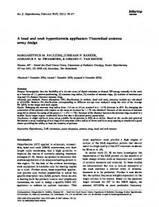
■ Figure 1. Multipath propagation channel: a) side view; b) top view.

around objects, and signal scattering. The result of these complex interactions is the presence of many signal components, or multipath signals, at the receiver. Another property of wireless channels is the presence of Doppler shift, which is caused by the motion of the receiver, the transmitter, and/or any other objects in the channel. A simplified pictorial of the multipath environment with two mobile stations is shown in Fig. 1. Each signal component experiences a different path environment, which will determine the amplitude A l,k, carrier phase shift ϕl,k, time delay τl,k, AOA θl,k, and Doppler shift fd of the lth signal component of the kth mobile. In general, each of these signal parameters will be time-varying. The early classical models, which were developed for narrowband transmission systems, only provide information about signal amplitude level distributions and Doppler shifts of the received signals. These models have their origins in the early days of cellular radio [1–4] when wideband digital modulation techniques were not readily available. As cellular systems became more complex and more accurate models were required, additional concepts, such as time delay spread, were incorporated into the model. Representing the RF channel as a time-variant channel and using a baseband complex envelope representation, the channel impulse response for mobile 1 has classically been represented as [5] h1 (t, τ) =

L(t ) – 1

∑

l=0

Al,1 (t )e

jϕ l ,1 ( t )

(

)

δ t – τ l,1 (t )

(1)

where L(t) is the number of multipath components and the other variables have already been defined. The amplitude Al,k of the multipath components is usually modeled as a Rayleigh distributed random variable, while the phase shift ϕl,k is uniformly distributed. The time-varying nature of a wireless channel is caused by the motion of objects in the channel. A measure of the time rate of change of the channel is the Doppler power spectrum, introduced by M. J. Gans in 1972 [2]. The Doppler power spectrum provides us with statistical information on the variation of the frequency of a tone received by a mobile traveling at speed v. Based on the flat fading channel model developed by R. H. Clarke in 1968, Gans assumed that the received signal at the mobile station came from all directions and was uniformly distributed. Under these assumptions and for a λ/4 vertical antenna, the Doppler power spectrum is given by [5] 1.5   2  f – fc   S ( f ) =  πf m 1 –    fm    0 

f – fc < f m

elsewhere

IEEE Personal Communications • February 1998

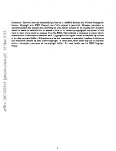
where fm is the maximum Doppler shift given by v/λ where λ is the wavelength of the transmitted signal at frequency fc. Figure 2 shows the received signals at the base station, assuming that mobiles 1 and 2 have transmitted narrow pulses at the same time. Also shown is the output of an antenna array system adapted to mobile 1. The channel model in Eq. 1 does not consider the AOA of each multipath component shown in Figs. 1 and 2. For narrowband signals, the AOA may be included into the vector channel impulse response using L(t ) – 1 r r h1 (t, τ) = ∑ Al,1 (t )e jϕ l (t ) a (θ l (t ))δ(t – τ l (t ))

(2)

l=0

where→ a (θl(t)) is the array response vector. The array response vector is a function of the array geometry and AOA. Figure 3 shows the case for an arbitrary array geometry when the array and signal are restricted to two-dimensional space. The resulting array response vector is given by

( – jψ l,1 )  ( – jψ l, 2 )  ( – jψ l,3 ) 

exp  exp   a(θ l (t )) = exp L  exp 

( – jψ l , m )

   

where ψl,i(t) =[xicos(θl(t)) + yisin(θl(t))]β and β = 2π/λ is the wavenumber. The spatial channel impulse response given in Eq. 2 is a summation of several multipath components, each of which has its own amplitude, phase, and AOA. The distribution of these parameters is dependent on the type of environment. In particular, the angle spread of the channel is known to be a function of both the environment and the base station antenna heights. In the next section, we describe macrocell and microcell environments and discuss how the environment affects the signal parameters.

Macrocell vs. Microcell Macrocell Environment — Figure 4 shows the channel on the forward link for a macrocell environment. It is usually assumed that the scatterers surrounding the mobile station are about the same height as or are higher than the mobile. This implies that the received signal at the mobile antenna arrives from all directions after bouncing from the surrounding scatterers as illustrated in Fig. 4. Under these conditions, Gans’ assumption that the AOA is uniformly distributed over [0, 2π] is valid. The classical

11

Received signal θ0,1

Mobile 1 θ1,1

τ0,1

τ1,1

θ2,1

τ2,1

Received signal

Received signal

Delay

(a) Received signal (c)

Mobile 2

θ0,2

Delay

(d)

Delay

θ1,2

τ0,2

τ1,2

Delay

(b)

■ Figure 2. Channel impulse responses for mobiles 1 and 2: a) received signal from mobile 1 to the base station; b) received signal from mobile 2 to the base station; c) combined received signal from mobiles 1 and 2 at the base station; d) received signal at the base station when a beam steered toward mobile 1 is employed.

Microcell Environment — In the microRayleigh fading envelope with deep cell environment, the base station fades approximately λ/2 apart Plane wave antenna is usually mounted at the same emanates from this model [5]. height as the surrounding objects. This However, the AOA of the received implies that the scattering spread of signal at the base station is quite difthe AOA of the received signal at the ferent. In a macrocell environment, (x1, y1) θ base station is larger than in the typically, the base station is deployed macrocell case since the scattering prohigher than the surrounding scatterx cess also happens in the vicinity of the ers. Hence, the received signals at base station. Thus, as the base station the base station result from the scatantenna is lowered, the tendency is for tering process in the vicinity of the the multipath AOA spread to increase. mobile station, as shown in Fig. 5. (x2, y1) (xm, ym) This change in the behavior of the The multipath components at the received signal is very important as far base station are restricted to a smallas antenna array applications are coner angular region, θ BW , and the dis■ Figure 3. Arbitrary antenna array cerned. Studies have shown that statistribution of the AOA is no longer configuration. tical characteristics of the received uniform over [0,2π]. Other AOA dissignal are functions of the angle tributions are considered later in this spread. Lee [3] and Adachi [6] found that the correlation article. between the signals received at two base station antennas The base station model of Fig. 5 was used to develop the increases as the angle spread decreases. theory and practice of base station diversity in today’s cellular This section has presented some of the physical properties system and has led to rules of thumb for the spacing of diverof a wireless communication channel. A mathematical expressity antennas on cellular towers [3]. sion that describes the time-varying spatial channel impulse response was given in Eq. 2. In the next section, several models that provide varying levels of information about the spatial channel are presented. Mobile station

Space: The Final Frontier

Mobile station Base station

Details of the Spatial Channel Models Top view Base station

■ Figure 4. Macrocell environment — the mobile station perspective.

12

In the past when the distribution of angle of arrival of multipath signals was unknown, researchers assumed uniform distribution over [0, 2π] [7]. In this section, a number of more realistic spatial channel models are introduced. The defining equations (or geometry) and the key results for the models

IEEE Personal Communications • February 1998

Top view

angle spreads and element spacings result are described. Also provided is an extenin lower correlations, which provide an sive list of references. Mobile station increased diversity gain. Measurements of Table 1 lists some representative active the correlation observed at both the base research groups in the field and their Web station and the mobile are consistent with site addresses where more information on a narrow angle spread at the base station the subject can be found. (Note that this is and a large angle spread at the mobile. by no means an exhaustive list.) Correlation measurements made at the The Gaussian Wide Sense Stationary base station indicate that the typical radius Uncorrelated Scattering (GWSSUS), θBW of scatterers is from 100 to 200 wave Gaussian Angle of Arrival (GAA), Typilengths [3]. cal Urban (TU), and Bad Urban (BU) Base station Assuming that N scatterers are uniformmodels described below were developed ly placed on the circle with radius R and in a series of papers at the Royal Institute ■ Figure 5. Macrocell — base oriented such that a scatterer is located on of Technology and may be downloaded station perspective. the line of sight, the discrete AOAs are [9] from the Web site. Further details of the Geometrically Based Single Bounce R 2π  θ i ≈ sin  i for i = 0,1,K, N – 1. (GBSB) models are given in theses at VirD  N  ginia Tech, which are available at http://etd.vt.edu/etd/ From the discrete AOAs, the correlation of the signals index.html. between any two elements of the array can be found using [9] These various models were developed and used for different applications. Some of the models were intended to pro1 N –1 ρ( d , θ 0 , R, D) = vide information about only a single channel characteristic, ∑ exp – j 2 πd cos(θ 0 + θ i ) , N i=0 such as angle spread, while others attempt to capture all the where d is the element spacing and θ0 is measured with respect properties of the wireless channel. In the discussion of the models, an effort is made to identify the original motivation of to the line between the two elements as shown in Fig. 6. the model and to convey the information the model is intendThe original model provided information regarding only ed to provide. signal correlations. Motivated by the need to consider smallscale fading in diversity systems, Stapleton et al. proposed an Lee’s Model extension to Lee’s model that accounts for Doppler shift by imposing an angular velocity on the ring of scatterers [10, 11]. In Lee’s model, scatterers are evenly spaced on a circular ring For the model to give the appropriate maximum Doppler about the mobile as shown in Fig. 6. Each of the scatterers is shift, the angular velocity of the scatterintended to represent the effect of many ers must equal v/R where v is the vehiscatterers within the region, and hence y cle velocity and R is the radius of the are referred to as effective scatterers. The scatterer ring [11]. Using this model to model was originally used to predict the Mobile simulate a Rayleigh fading spatial chancorrelation between the signals received Effective scatterers nel model, the BER for a π/4 differenby two sensors as a function of element tial quadrature phase shift keyed spacing. However, since the correlation R D (DQPSK) signal was simulated. The matrix of the received signal vector of results were compared with measurean antenna array can be determined by ments taken in a typical suburban enviconsidering the correlation between θBW ronment. The resulting BER estimates each pair of elements, the model has θ0 were within a factor of two of the actual application to any arbitrary array size. x measured BER, indicating a reasonable The level of correlation will deterd Base station degree of accuracy for the model [10]. mine the performance of spatial diversiWhen the model is used to provide ty methods [3, 9]. In general, larger ■ Figure 6. Lee’s model.

[

]

Research group

Web site

Center for Communications Research — University of Bristol

http://www.fen.bris.ac.uk/elec/research/ccr/ccr.html

Center for Personkommunikation — Aalborg University

http://www.kom.auc.dk/CPK/

Center for Wireless Telecommunications — Virginia Tech

http://www.cwt.vt.edu/

Mobile and Portable Radio Research Group — Virginia Tech

http://www.mprg.ee.vt.edu

Research Group for RF Communications — University of Kaiserlautern

http://www.e-technik.uni-kl.de/

Royal Institute of Technology

http://www.s3.kth.se

Smart Antenna Research Group — Stanford University

http://www-isl.stanford.edu/groups/SARG

Telecommunications and Information Systems Engineering — University of Texas at Austin

http://www.ece.utexas.edu/projects/tise/

Wireless Technology Group — McMaster University

http://www.crl.mcmaster.ca

■ Table 1. Some active research groups in the field of adaptive antenna arrays.

IEEE Personal Communications • February 1998

13

y

tributed (see the discussion of the GAA joint AOA and time of arrival (TOA) D model later). However, in practice the channel information, one finds that the Effective AOA will be discrete (i.e., a finite numresulting power delay profile is “Uscatterers ber of samples from a Gaussian distribushaped” [12]. By considering the intertion), and therefore it is not valid to use sections of the effective scatterers by θBW a continuous AOA distribution to estiellipses of constant delay, one finds that θ0 x mate the correlation present between there is a high concentration of scatterdifferent antenna elements in the array. ers in ellipses with minimum delay, a Base station d The correlation that results from a conhigh concentration of scatterers in tinuous AOA distribution decreases ellipses with maximum delay, and a ■ Figure 7. Discrete uniform geometry. monotomically with element spacing, lower concentration of scatterers whereas the correlation that results between. Higher concentrations of from a discrete AOA has damped scatterers with a given delay correScatterer region oscillations present. Therefore, a conspond with larger powers, and hence y tinuous AOA distribution will underlarger values on the power delay proestimate the correlation that exists file. The “U-shaped” power delay Mobile between the elements in the array [9]. profile is not consistent with measureD x In [9], a comparison is made ments. Therefore, an extension to Base between the correlation obtained Lee’s model is proposed in [11] in station Rm using the discrete uniform distribution which additional scatterer rings are model, Lee’s model, and a continuous added to provide different power Gaussian AOA as a function of eledelay profiles. ■ Figure 8. Circular scatterer density geometry. ment spacing. The comparisons indiWhile the model is quite useful in cate that, for small element predicting the correlation between any separations (two wavelengths), the two elements of the array, and hence three models have nearly identical correlations. For larger elethe array correlation matrix, it is not well suited for simulament separations (greater than two wavelengths), the correlations requiring a complete model of the wireless channel. tion values using the continuous Gaussian AOA are close to Discrete Uniform Distribution zero, while the two discrete models have oscillation peaks with correlations as high as 0.2 even beyond four wavelengths. A model similar to Lee’s model in terms of both motivation Additionally, it was found that the correlation of the discrete and analysis was proposed in [9]. The model (referred to here uniform distribution falls off more quickly than the correlaas the discrete uniform distribution) evenly spaces N scattertion in Lee’s model. ers within a narrow beamwidth centered about the line of Again, while the model is useful for predicting the correlasight to the mobile as shown in Fig. 7. The discrete possible tion between any pair of elements in the array (which can be AOAs, assuming N is odd, are given by [9] used to calculate the array correlation matrix), it fails to 1 N –1 N –1 ,K, . θi = θ BW i, i = – include all the phenomena, such as delay spread and Doppler N –1 2 2 spread, required for certain types of simulations. From this, the correlation of the signals present at two antenna elements with a separation of d is found to be Geometrically Based Single-Bounce 1 ρ( d , θ 0 , θ BW ) = N

N –1 2

∑

i=–

N –1 2

[

Statistical Channel Models

]

exp – j 2 πd cos(θ 0 + θ i ) .

Probability density [log 10(f)]

Probability density [log 10(f)]

Measurements reported in [9] suggest that the AOA statistics in rural and suburban environments are Gaussian dis-

2 1.5 1 0.5 0 –0.5 –1 5 0

–5 Angle of arrival (degrees)

3.9 3.7 3.8 3.6 3.4 3.5 Time of arrival (µs)

4

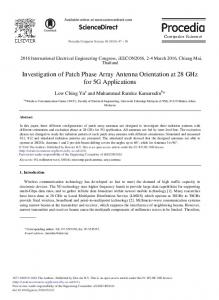
■ Figure 9. Joint TOA and AOA probability density function at the base station, circular model (log-scale).

14

Geometrically Based Single-Bounce (GBSB) Statistical Channel Models are defined by a spatial scatterer density function. These models are useful for both simulation and analysis purposes. Use of the models for simulation involves randomly placing scatterers in the scatterer region according to the form 2 0 –2 –4 –6 100 0 –100 Angle of arrival (degrees)

3.7

3.4 3.5

3.8

3.9

4

3.6 Time of arrival (µs)

■ Figure 10. Joint TOA and AOA probability density function at the mobile, circular model (log-scale).

IEEE Personal Communications • February 1998

y Scatterer region

bm

D x MHz, which provides a range of of the spatial scatterer density 30–60 m, roughly the width of function. From the location of Base station Mobile wide urban streets. each of the scatterers, the AOA, The GBSBCM can be used to TOA, and signal amplitude are am generate random channels for determined. simulation purposes. Generation From the spatial scatterer den■ Figure 11. Elliptical scatterer density geometry. of samples from the GBSBCM is sity function, it is possible to derive accomplished by uniformly placthe joint and marginal TOA and ing scatterers in the circular scatterer region about the mobile AOA probability density functions. Knowledge of these statisand then calculating the corresponding AOA, TOA, and tics can be used to predict the performance of an adaptive power levels. array. Furthermore, knowledge of the underlying structure of the resulting array response vector may be exploited by beamGeometrically Based Elliptical Model (Microcell Wideband forming and position location algorithms. Model) — The Geometrically Based Single Bounce Elliptical The shape and size of the spatial scatterer density function Model (GBSBEM) assumes that scatterers are uniformly disrequired to provide an accurate model of the channel is subtributed within an ellipse, as shown in Fig. 11, where the base ject to debate. Validation of these models through extensive station and mobile are the foci of the ellipse. The model was measurements remains an active area of research. proposed for microcell environments where antenna heights are relatively low, and therefore multipath scattering near the Geometrically Based Circular Model (Macrocell Model) — The base station is just as likely as multipath scatterering near the geometry of the Geometrically Based Single Bounce Circular mobile [17, 18]. Model (GBSBCM) is shown in Fig. 8. It assumes that the scatA nice attribute of the elliptical model is the physical interterers lie within radius Rm about the mobile. Often the requirepretation that only multipath signals which arrive with an ment that R m < D is imposed. The model is based on the absolute delay ≤ τm are accounted for by the model. Ignoring assumption that in macrocell environments where antenna heights are relatively large, there will be no signal scatterering components with larger delays is possible since signals with from locations near the base station. The idea of a circular longer delays will experience greater path loss, and hence region of scatterers centered about the mobile was originally have relatively low power compared to those with shorter proposed by Jakes [13] to derive theoretical results for the cordelays. Therefore, provided that τ m is chosen sufficiently relation observed between two antenna elements. Later, it was large, the model will account for nearly all the power and used to determine the effects of beamforming on the Doppler AOA of the multipath signals. spectrum [14, 15] for narrowband signals. It was shown that The parameters a m and b m are the semimajor axis and the rate and the depth of the envelope fades are significantly semiminor axis values, which are given by cτ reduced when a narrow-beam beamformer is used. am = m , The joint TOA and AOA density function obtained from 2 the model provides some insights into the properties of the 1 2 2 bm = c τ m – D2 , model. Using a Jacobian transformation, it is easy to derive 2 the joint TOA and AOA density function at both the base station and the mobile. The resulting joint probability density functions (PDFs) at the At the base station: base station and the mobile are shown in the box on this page [16]. fτ, θ b ( τ, θ b ) = The joint TOA and AOA PDFs for the GBSBCM are shown in Figs. 9 and 10 for  D 2 – τ 2 c 2 D 2 c + τ 2 c 3 – 2 τc 2 D cos(θ ) D 2 – 2 τcD cos(θ b ) + τ 2 c 2 b the case of D = 1 km and R m = 100 m  : ≤ 2 Rm 3 from the base station and mobile perspec τc – D cos(θ b ) 4 πRm2 D cos(θ b ) – τc  tives, respectively. The circular model pre dicts a relatively high probability of  multipath components with small excess  : 0 else.  delays along the line of sight. From the  base-station perspective, all of the multipath components are restricted to lie with in a small range of angles. At the mobile: The appropriate values for the radius of scatterers can be determined by equatfτ, θ m ( τ, θ m ) = ing the angle spread predicted by the model (which is a function of R m ) with  D 2 – τ 2 c 2 D 2 c + τ 2 c 3 – 2 τc 2 D cos(θ ) m D2 – τ 2 c 2 measured values. Measurements reported  : ≤ 2 Rm 3  in [9] suggest that typical angle spreads D cos(θ m ) – τc 4 πRm2 D cos(θ m ) – τc  for macrocell environments with a T-R  separation of 1 km are approximately two   to six degrees. Also, it is stated that the : else, 0  angle spread is inversely proportional to  the T-R separation, which leads to a  radius of scatterers that ranges from 30 to where θb and θm are the angle of arrival measured relative to the line of sight 200 m [16]. In [3], it is stated that the from the base station and the mobile, respectively. active scattering region around the mobile is about 100–200 wavelengths for 900

IEEE Personal Communications • February 1998

(

)(

(

)(

(

(

)

)

)

)

15

Probability density [log 10(f)]

–1 –2 –3 –4 –5 –6 –7

GWSSUS. Figure 13 shows the geometry assumed for the GWSSUS model corresponding to d = 3 clusters. The mean AOA for the kth cluster is denoted θ0k. It is assumed that the location and delay associated with each cluster remains constant over several data bursts, b. The form of the received signal vector is

100 0 –100

4.5

4

3.5

Angle of arrival (degrees)

5

Time of arrival (µs)

■ Figure 12. Joint TOA and AOA probability density function, elliptical model (log-scale).

x b (t ) =

(

)(

)

 D 2 – τ 2 c 2 D 2 c + τ 2 c 3 – 2 τc 2 D cos(θ ) b D  ≤ τ ≤ τm 3 c  4 πam bm D cos(θ b ) – τc   0 elsewhere, where θb is AOA observed at the base station. A plot of the joint TOA and AOA PDF is shown in Fig. 12 for the case of D = 1 km and τm = 5 µs. From the plot of the joint TOA and AOA PDF, it is apparent that the GBSBEM results in a high probability of scatterers with minimum excess delay along the line of sight. The choice of τm will determine both the delay spread and angle spread of the channel. Methods for selecting an appropriate value of τm are given in [18]. Table 2 summarizes the techniques for selecting τm where Lr is the reflection loss in dB, n is the path loss exponent, and τ0 is the minimum path delay. To generate multipath profiles using the GBSBEM, the most efficient method is to uniformly place scatterers in the ellipse and then calculate the corresponding AOA, TOA, and power levels from the coordinates of the scatterer. Uniformly placing scatterers in an ellipse may be accomplished by first uniformly placing the scatterers in a unit circle and then scaling each x and y coordinate by am and bm, respectively [16].

(

)

k =1

where vk,b is the superposition of the steering vectors during the bth data burst within the kth cluster, which may be expressed as v k,b =

where c is the speed of light and τm is the maximum TOA to be considered. To gain some insight into the properties of this model, consider the resulting joint TOA and AOA density function. Using a transformation of variables of the original uniform scatterer spatial density function, it can be shown that the joint TOA and AOA density function observed at the base station is given by [16] fτ, θ b ( τ, θ b ) =

d

∑ v k , b s(t – τ k ),

Nk

∑ α k,i e

jφ k ,i

i =1

(

)

a θ 0k – θ k,i ,

where Nk denotes the number of scatterers in the kth cluster, αk,i is the amplitude, φk,j is the phase, θk,i is the angle of arrival of the ith reflected scatterer of the kth cluster, and a(θ) is the array response vector in the direction of θ [9]. It is assumed that the steering vectors are independent for different k. If Nk is sufficiently large (approximately 10 or more [19]) for each cluster of scatterers, the central limit theorem may be applied to the elements of vk,b. Under this condition, the elements of v k,b are Gaussian distributed. Additionally, it is assumed that vk,b is wide sense stationary. The time delays τk are assumed to be constant over several bursts, b, whereas the phases φ k,i change much more rapidly. The vectors v k,b are assumed to be zero mean, complex Gaussian wide sense, stationary random processes where b plays the role of the time argument. The vector vk,b is a multivariate Gaussian distribution, which is described by its mean and covariance matrix. When no line of sight component is present, the mean will be zero due to the random phase φ k,i , which is assumed to be uniformly distributed in the range 0 to 2π. When a direct path component is present, the mean becomes a scaled version of the corresponding array response vector E{vk,b} ∝ a(θ0k) [9]. The covariance matrix for the kth cluster is given by [21]

{

} E{a(θ

Rk = E v k , b v kH, b =

Nk

∑ α k,i

i =1

2

0k

) (

)}

– θ k,i a H θ 0k – θ k,i .

The model provides a fairly general result for the form of the covariance matrix. However, it does not indicate the number or location of the scattering clusters, and hence requires some additional information for application to typical environments.

Gaussian Angle of Arrival

The Gaussian Angle of Arrival (GAA) channel model is a Gaussian Wide Sense Stationary special case of the GWSSUS model described above where Uncorrelated Scattering only a single cluster is considered (d = 1), and the AOA statistics are assumed to be Gaussian distributed about some The GWSSUS is a statistical channel model that makes nominal angle, θ0, as shown in Fig. assumptions about the form of the received signal vector [19–22]. The primary motivation of 14. Since only a single cluster is conthe model is to provide a general sidered, the model is a narrowband Criteria Expression equation for the received signal corchannel model that is valid when relation matrix. In the GWSSUS the time spread of the channel is Fixed maximum delay, τm τm = constant model, scatterers are grouped into small compared to the inverse of clusters in space. The clusters are the signal bandwidth; hence, time (T – Lr)/10n Fixed threshold T in dB τm = τ010 such that the delay differences withshifts may be modeled as simple in each cluster are not resolvable phase shifts [23]. Fixed delay spread, σt τm = 3.244στ + τ0 within the transmission signal bandThe statistics of the steering vecwidth. By including multiple clustor are distributed as a multivariate Fixed max. excess delay, τe τm = τ0 + τe ters, frequency-selective fading Gaussian random variable. Similar ■ Table 2. Methods for selection τm. channels can be modeled using the to the GWSSUS model, if no line of

16

IEEE Personal Communications • February 1998

y

y

Scatterer cluster

kth scatterer cluster

θ0k

θ0k

x

Base station

x

bution in all directions away from the mobile [24]. Both the time and spatial correlation properties of the model are compared to theoretical results in [24]. The comparison shows that there is good agreement between the two.

Two Simulation Models (TU and BU)

Base station

Next we describe two spatial channel models ■ Figure 13. GWSSUS geometry. ■ Figure 14. GAA geometry. that have been developed for simulation purposes. The Typical Urban (TU) model is designed to have time properties similar to the GSM-TU defined in sight is present, then E{vk,b} = 0; otherwise, the mean is proGSM 05.05, while the Bad Urban (BU) model was developed portional to the array response vector a(θ0k). For the special to model environments with large reflectors that are not in case of uniform linear arrays, the covariance matrix may be the vicinity of the mobile. Although the models are designed described by for GSM, DCS1800, and PCS1900 formats, extensions to H R(θ 0 , σ θ ) ≈ pa(θ 0 )a (θ 0 ) ⊗ B(θ 0 , σ θ ), other formats are possible [251]. Both of these models obtain the received signal vector where the (k,l) element of B(θ0, σθ) is given by using 2 2 B(θ 0 , σ θ ) kl = exp –2( π∆( k – l )) σ θ cos 2 θ , N l (t )    l (t )  x(t ) = α n (t ) exp – j 2πfc n + β  s t – n + ∆ t  a(θ n (t )) p is the receiver signal power, ∆ is the element spacing, and ⊗    c  c n =1 denotes element-wise multiplication [23]. where N is the number of scatterers, fc the carrier frequency, c is the speed of light, ln(t) the path propagation distance, β a Time-Varying Vector random phase, and ∆ t random delay. In general, the path Channel Model (Raleigh’s Model) propagation distance l n(t) will vary continuously with time; hence, Doppler fading occurs naturally in the model. Raleigh’s time-varying vector channel model was developed to provide both small scale Rayleigh fading and theoretical spaTypical Urban (TU) — In the TU model, 120 scatterers are rantial correlation properties [24]. The propagation environment domly placed within a 1 km radius about the mobile [25]. The considered is densely populated with large dominant reflecposition of the scatterers is held fixed over the duration in tors (Fig. 15). It is assumed that at a particular time the chanwhich the mobile travels a distance of 5 m. At the end of the 5 nel is characterized by L dominant reflectors. The received m, the scatterers are returned to their original position with signal vector is then modeled as L(t ) – 1 respect to the mobile. At each 5-m interval, random phases are x(t ) = ∑ a(θ l )α l (t )s(t – τ ) + n(t ), assigned to the scatterers as well as randomized shadowing l=0 effects, which are modeled as log-normal with distance with a standard deviation of 5–10 dB [25]. The received signal is where a is the array response vector, αl(t) is the complex path determined by brute force from the location of each of the scatamplitude, s(t) is the modulated signal, and n(t) is additive terers. An exponential path loss law is also applied to account noise. This is equivalent to the impulse response given in Eq. 2. for large-scale fading [21]. Simulations have shown that the TU The unique feature of the model is in the calculation of model and the GSM-TU model have nearly identical power the complex amplitude term, al(t), which is expressed as delay profiles, Doppler spectrums, and delay spreads [25]. Furα1 (t ) = β l (t ) ⋅ Γl ⋅ ψ ( τ l ) , thermore, the AOA statistics are approximately Gaussian and similar to those of the GAA model described above. where Γl accounts for log-normal fading, ψ(τl) describes the power delay profile, and βl(t) is the complex intensity of the Bad Urban (BU) — The BU is identical to the TU model with radiation pattern as a function of time. The complex intensity the addition of a second scatterer cluster with another 120 is described by Nl scatterers offset 45˚ from the first, as shown in Fig. 16. The scatterers in the second cluster are assigned 5 dB less average β l (t ) = K ∑ Cn (θ l ) exp jω d cos Ω n, l t , power than the original cluster [25]. The presence of the secn =1 ond cluster results in an increased where N l is the number of signal angle spread, which in turn components contributing to the lth reduces the off-diagonal elements dominant reflecting surface, K Dominant of the array covariance matrix. accounts for the antenna gains reflectors The presence of the second cluster and transmit signal power, Cn(θl) also causes an increase in the delay is the complex radiation of the nth spread. component of the lth dominant reflecting surface in the direction Uniform Sectored Distribution of θl, ωd is the maximum Doppler shift, and Ωn,l is the angle toward The defining geometry of Uniform the nth component of the lth domSectored Distribution (USD) is Base station inant reflector with respect to the shown in Fig. 17 [26]. The model Local scatterers motion of the mobile. The resultassumes that scatterers are uniing complex intensity, β l (t), formly distributed within an angle distribution of θ BW and a radial exhibits a complex Gaussian distri■ Figure 15. Raleigh’s model signal environment.

[

]

(

(

∑

))

IEEE Personal Communications • February 1998

17

Secondary cluster

range of ∆R centered about the mobile. The magnitude and phase associated with each scatterer is selected at random from a uniform distribution of [0,1] and [0, 2π], respectively. As the number of scatterers approaches infinity, the signal fading envelope becomes Rayleigh with uniform phase [26]. In [26], the model is used to study the effect of angle spread on spatial diversity techniques. A key result is that beam-steering techniques are most suitable for scatterer distributions with widths slightly larger than the beamwidths.

Modified Saleh-Valenzuela’s Model

mation was developed by Klein and Mohr [29]. The channel impulse response is represented by

Base station

h( τ, t, θ) =

W

∑ aw (t )δ(τ – τ w )δ(θ – θ w ).

w =1

This model is composed by W taps, each with an associated time delay τ w , complex amplitude αw, and AOA θw. The ■ Figure 16. Bad Urban vector chanjoint density functions of the model nel model geometry. parameters should be determined from measurements. As shown in [29], measurements can provide histograms of the joint distribution of |a|, τ, and θ, and the density functions, which are proportional to these histograms, can be chosen. Primary cluster

Elliptical Subregions Model (Lu, Lo, and Litva’s Model)

Saleh and Valenzuela developed a multipath channel model for indoor environment based on the clustering phenomenon observed in experimental data [27]. The clustering phenomenon refers to the observation that multipath components arrive at the antenna in groups. It was found that both the clusters and the rays within a cluster decayed in amplitude with time. The impulse response of this model is given by

Lu et al. [30] proposed a model of multipath propagation based on the distribution of the scatterers in elliptical subregions, as shown in Fig. 18. Each subregion (shown in a different shade) corresponds to one range of the excess delay time. This approach is similar to the GBS∞ ∞ h(t ) = ∑ ∑ α ij δ t – Ti – τ ij (3) BEM proposed by Liberti and Rappay i=0j =0 port [18] in that an ellipse of scatterers where the sum over i corresponds to is considered. The primary difference the clusters and the sum over j reprebetween the two models is in the selec∆R sents the rays within a cluster. The varition of the number of scatterers and the ables α ij are Rayleigh distributed with distribution of those scatterers. In the GBSBEM, the scatterers were uniformly the mean square value described by a distributed within the entire ellipse. In double-exponential decay given by Lu, Lo, and Litva’s model, the ellipse is Multipath region α ij2 = α 200 exp( – Ti / Γ ) exp τ ij / γ first subdivided into a number of elliptical subregions. The number of scatterers θBW within each subregion is then selected where Γ and γ are the cluster and ray from a Poisson random variable, the time decay constant, respectively. Motiθ0 x mean of which is chosen to match the vated by the need to include AOA in measured time delay profile data. the channel mode, Spencer et al. proBase station It was also assumed that the multiposed an extension to the Saleh-Valenpath components arrive in clusters due zuela’s model [28], assuming that time ■ Figure 17. Geometry of the uniform to the multiple reflecting points of the and the angle are statistically indepensectored distribution. scatterers. Thus, assuming that there dent, or are L scatterers with Kl reflecting points h(t,θ) = h(t)h(θ). each, the model proposed is represented by Similar to the time impulse response in Eq. 3, the proL t posed angular impulse response is given by h(t, t 0 ) = Et θ i( )

(

)

(

h(t ) =

)

i=0j =0

where αij is the amplitude of the jth ray in the ith cluster. The variable Θi is the mean angle of the ith cluster and is assumed to be uniformly distributed over [0, 2π]. The variable ωij corresponds to the ray angle within a cluster and is modeled as a Laplacian distributed random variable with zero mean and standard deviation σ: f (ω ) =

 1 2ω  exp – . σ  2σ 

This model was proposed based on indoor measurements which will be discussed in the fourth section.

Extended Tap-Delay-Line Model A wideband channel model that is an extension of the traditional statistical tap-delay-line model and includes AOA infor-

18

∑ ( )

∞ ∞

∑ ∑ α ij δ(θ – Θ i – ω ij )

i =1 Ki

×

∑α k =0

ik

(

)

exp – (2πfik t 0 + γ ik ) δ (t – τ ik ) Er (θ ik )

where αik, τik, and γik correspond to the amplitude, time delay, and phase of the signal component from the ikth reflecting point, respectively. fik is the Doppler frequency shift of each individual path, θik is the angle between the ikth path and the (t) receiver-to-transmitter direction, and θi is the angle of the ith scatterer as seen from the transmitter. Et(θ) and Er(θ) are the radiation patterns of the transmit and receive antennas, respectively. The variable θik was assumed to be Gaussian distributed. Simulation results using this model were presented in [30], showing that a 60° beamwidth antenna reduces the mean RMS delay spread by about 30–43 percent. These results are consistent with similar measurements made in Toronto using a sectorized antenna [31].

IEEE Personal Communications • February 1998

Measurement-Based Channel Model

• By using directional antennas, it is possible to reduce the time dispersion. Another set of TOA and AOA measurements is reported in [39] for urban areas. The measurements were made using a A channel model in which the parameters are based on meatwo-element receiver that was mounted on the test vehicle surement was proposed by Blanz et al. [32]. The idea behind with an elevation of 2.6 m. The transmitting antenna was this approach is to characterize the propagation environment, placed 30 m high on the side of a building. A bandwidth of 10 in terms of scattering points, based on measurement data. The MHz with a carrier frequency of 2.33 GHz was used. The time-variant impulse response takes the form delay-Doppler spectra observed at the mobile was used to 2π obtain the delay-AOA spectra. The second antenna element is h( τ, t ) = ∫ ϑ( τ, t, θ) * g( τ, θ) * f ( τ)dθ used to remove the ambiguity in AOA that would occur if 0 only the Doppler spectra were known. The results indicate that it is possible to account for most of the major features of where f(τ) is the impulse response representing the joint the delay-AOA spectra by considering the large buildings in transfer characteristic of the transmission system components the environment. (modulator, demodulator, filters, etc.), and g(τ, θ) is the charMotivated by diversity combining methods, earlier meaacteristic of the base station antenna. The term ϑ (τ, t, θ) is surements were concerned primarily with determining the the time-variant directional distribution of channel impulse correlation between the signals at two antenna elements as response seen from the base station. This distribution is timea function of the element separation distance. These studvariant due to mobile motion and depends on the location, ies found that, at the mobile, relatively small separation orientation, and velocity of the mobile station antenna and distances were required to obtain a small degree of correthe topographical and morphographical properties of the lation between the elements, whereas at the base station propagation area as well. Measurement is used to determine very large spacing was needed. the distribution ϑ (τ, t, θ). Thes e findings indicate that Ray Tracing Models there is a relatively small angle spread observed at the base staThe models presented so far are tion [6]. based on statistical analysis and Previously, an extension to measurements, and provide us Saleh-Valenzuela’s indoor model, with the average path loss and including AOA information, was delay spread, adjusting some presented. This extension was parameters according to the enviproposed based on indoor mearonment (indoor, outdoor, surements of delay spread and obstructed, etc.). In the past few AOA at 7 GHz made at Brigham years, a deterministic model, called Young University [40]. The ray tracing, has been proposed ■ Figure 18. Elliptical subregions spatial scatterer AOAs were measured using a 60 based on the geometric theory and density. cm parabolic dish antenna that reflection, diffraction, and scatterhad a 3 dB beamwidth of 6°. The ing models. By using site-specific results showed a clustering pattern in both time and angle information, such as building databases or architecture drawdomain, which led to the proposed channel model described ings, this technique deterministically models the propagation in [28]. Also, it was observed that the cluster mean angle of channel [33–36], including the path loss exponent and the arrival was uniformly distributed [0, 2π]. The distribution of delay spread. However, the high computational burden and the angle of arrival of the rays within a cluster presented a lack of detailed terrain and building databases make ray tracsharp peak at the mean, leading to the Laplacian distribuing models difficult to use. Although some progress has been tion modeling. The standard deviation found for this distrimade in overcoming the computational burden, the developbution was around 25°. Based on these measurements, a ment of an effective and efficient procedure for generating channel model including delay spread and AOA informaterrain and building data for ray tracing is still necessary. tion was proposed, supposing that time and angle were Channel Model Summary independent variables. In [41], two-dimensional AOA and delay spread meaTable 3 summarizes each of the spatial models presented above. surement and estimation were presented. The measurements were made in downtown Paris using a channel Spatial Signal Measurements sounder at 900 MHz and a horizontal rectangular planar array at the receiver. The estimation of AOA, including There have been only a few publications relating to spatial azimuth and elevation angle, was performed using 2D unichannel measurements. In this section, references are given to tary ESPRIT [42] with a time resolution of 0.1µs and angle these papers, and the key results are described. resolution of 5°. The results presented confirmed assumpIn [38], TOA and AOA measurements are presented for tions made in urban propagation, such as the wave-guiding outdoor macrocellular environments. The measurements were mechanism of streets and the exponential decay of the made using a rotating 9˚ azimuth beam directional receiver power delay profile. Also, it was observed that 90 percent of antenna with a 10 MHz bandwidth centered at 1840 MHz. the received power was contained in the paths with elevaThree environments near Munich were considered, including tion between 0° and 40° with the low elevated paths conrural, suburban, and urban areas with base station antenna tributing a larger amount. heights of 12.3 m, 25.8 m, and 37.5 m, respectively. The key Finally, in [43] measurements are used to show the variaobservations made include [38]: tion in the spatial signature with both time and frequency. • Most of the signal energy is concentrated in a small interval Two measures of change are given, the relative angle change of delay and within a small AOA in rural, suburban, and given by even many urban environments.

IEEE Personal Communications • February 1998

19

Model

Description

References

Lee’s Model

Effective scatterers are evenly spaced on a circular ring about the mobile Predicts correlation coefficient using a discrete AOA model Extension accounts for Doppler shift

[3, 9, 11]

Discrete Uniform Distribution

N scatterers are evenly spaced over an AOA range Predicts correlation coefficient using a discrete AOA model Correlation predicted by this model falls off more quickly than the correlation in Lee’s model

[9]

Geometrically Based Circular Model (Macrocell Model)

Assumes that the scatterers lie within circular ring about the mobile AOA, TOA, joint TOA and AOA, Doppler shift, and signal amplitude information is provided Intended for macrocell environments where antenna heights are relatively large

[12–14, 16, 37]

Geometrically Based Scatterers are uniformly distributed in an ellipse where the base station and the mobile Elliptical Model (Microcell are the foci of the ellipse Wideband Model) AOA, TOA, joint TOA and AOA, Doppler shift, and signal amplitude information is provided Intended for microcell environments where antenna heights are relatively low

[17, 18]

Gaussian Wide Sense Stationary Uncorrelated Scattering (GWSSUS)

N scatterers are grouped into clusters in space such that the delay differences within each cluster are not resolvable within the transmission signal BW Provides an analytical model for the array covariance matrix

[19–22]

Gaussian Angle of Arrival (GAA)

Special case of the GWSSUS model with a single cluster and angle of arrival statistics assumed to be Gaussian distributed about some nominal angle Narrowband channel model Provides an analytical model for the array covariance matrix

[23]

Time-Varying Vector Channel Model (Raleigh’s Model)

Assumes that the signal energy leaving the region of the mobile is Rayleigh faded Angle spread is accounted for by dominant reflectors Provides both Rayleigh fading and theoretical spatial correlation properties

[20]

Typical Urban

Simulation model for GSM, DCS1800, and PCS1900 Time domain properties are similar to the GSM-TU defined in GSM 05.05 120 scatterers are randomly placed within a 1 km radius about the mobile Received signal is determined by brute force from the location of each of the scatterers and the time-varying location of the mobile AOA statistics are approximately Gaussian

[21, 22, 25]

Bad Urban

Simulation model for GSM, DCS1800, and PCS1900 Accounts for large reflectors not in the vicinity of the mobile Identical to the TU model with the addition of a second scatterer cluster offset 45˚ from the first

[21, 22, 25]

Uniform Sectored Distribution

Assumes that scatterers are uniformly distributed within an angle distribution of θBW and a radial range of ∆R centered about the mobile Magnitude and phase associated with each scatterer are selected at random from a uniform distribution of [0,1] and [0, 2π], respectively

[26]

Modified SalehValenzuela’s Model

An extension to the Saleh-Valenzuela model, including AOA information in the channel model Assumes that time and the angle are statistically independent Based on indoor measurements

[28]

Extended Tap-Delay-Line Model

Wideband channel model Extension of the traditional statistical tap-delay-line model which includes AOA information The joint density functions of the model parameters should be determined from measurements

[29]

Spatio-Temporal Model Model of multipath propagation based on the distribution of the scatterers in elliptical (Lu, Lo, and Litva’s Model) subregions, corresponding to a range of excess delay time Similar to the GBSBEM

[30]

Measurement-Based Channel Model

Parameters are based on measurement Characterizes the propagation environment in terms of scattering points

[32]

Ray Tracing Models

Deterministic model based on the geometric theory and reflection, diffraction, and scattering models Uses site-specific information, such as building databases or architecture drawings

[33–36]

■ Table 3. Summary of spatial channel models.

20

IEEE Personal Communications • February 1998

Relative Angle Change (%) = 100 ×

1–

a *i ai

⋅

a *j

2

aj

and the relative amplitude change, found using Relative Amplitude Change(dB) = 20log10

aj ai

where ai and aj are the two spatial signatures (array response vectors) being compared. The measurements indicate that when the mobile and surroundings are stationary, there are relatively small changes in the spatial signature. Likewise, there are moderate changes when objects and the environment are in motion and large changes when the mobile itself is moving. Also, it was found that the spatial signature changes significantly with a change in carrier frequency. In particular, the measurements found that the relative amplitude change in the spatial signal could exceed 10 dB with a frequency change of only 10 MHz. This result indicates that the uplink spatial signature cannot be directly applied for downlink beamforming in most of today’s cellular and PCS systems that have 45 MHz and 80 MHz separation between the uplink and downlink frequencies, respectively.

Application of Spatial Channel Models The effect that classical channel properties such as delay spread and Doppler spread have on system performance has been an active area of research for several years and hence is fairly well understood. The spatial channel models include the AOA properties of the channel, which are often characterized by the angle spread. The angle spread has a major impact on the correlation observed between the pairs of elements in the array. These correlation values specify the received signal vector covariance matrix, which is known to determine the performance of linear combining arrays [44]. In general, the higher the angle spread the lower the correlation observed between any pair of elements in the array. The various spatial channel models provide different angle spreads and hence will predict different levels of system performance. The channel models presented here have various applications in the analysis and design of systems that utilize adaptive antenna arrays. Some of the models were developed to provide analytical models of the spatial correlation function, while others are intended primarily for simulation purposes.

Simulation More and more companies are relying on detailed simulations to help design and develop today’s wireless networks. The application of adaptive antennas is no exception. However, to obtain reliable results, accurate spatial channel models are needed. With accurate simulations of adaptive antenna array systems, researchers will be able to predict the capacity improvement, range extension, and other performance measures of the system, which in turn will determine the cost effectiveness of adaptive array technologies.

Algorithm Development The availability of channel models also opens up the possibility of developing new maximum likelihood smart antennas and AOA estimation algorithms based on these channel models. Good analytical models that will provide insights into the structure of the spatial channel are needed.

IEEE Personal Communications • February 1998

Conclusions As antenna technology advances, radio system engineers are increasingly able to utilize the spatial domain to enhance system performance by rejecting interfering signals and boosting desired signal levels. However, to make effective use of the spatial domain, design engineers need to understand and appropriately model spatial domain characteristics, particularly the distribution of scatterers, angles of arrival, and the Doppler spectrum. These characteristics tend to be dependent on the height of the transmitting and receiving antennas relative to the local environment. For example, the distributions expected in a microcellular environment with relatively low base station antenna heights are usually quite different from those found in traditional macrocellular systems with elevated base station antennas. This article has provided a review of a number of spatial propagation models. These models can be divided into three groups: • General statistically based models • More site-specific models based on measurement data • Entirely site-specific models. The first group of models (Lee’s Model, Discrete Uniform Distribution Model, Geometrically Based Single Bounce Statistical Model, Gaussian Wide Sense Stationary Uncorrelated Scattering Model, Gaussian Angle of Arrival Model, Uniform Sectored Distributed Model, Modified Saleh-Valenzuela’s Model, Spatio-Temporal Model) are useful for general system performance analysis. The models in the second group (Extended Tap Delay Line Model and Measurement-Based Channel Model) can be expected to yield greater accuracy but require measurement data as an input. An example from the third group of models is Ray Tracing, which has the potential to be extremely accurate but requires a comprehensive description of the physical propagation environment as well as measurements to validate the models. Further research is required to validate and enhance the models described in this article. Bearing in mind that an objective of modeling is to substantially reduce the amount of physical measurement required in the system planning process, it is important for design engineers to have reliable models of AOA, TDOA, delay spread, and the power of the multipath components. Further measurement programs that focus on spatial domain signal characteristics are required. These programs would greatly benefit from the development of improved measurement equipment. Armed with improved spatial channel modeling tools and a greater understanding of signal propagation, engineers can begin to meet the challenges inherent in designing future high-capacity/high-quality wireless communication systems, including the effective use of smart antennas.

References [1] R. H. Clarke, “A Statistical Theory of Mobile-Radio Reception,” Bell Sys. Tech. J., vol. 47, 1968, pp. 957–1000. [2] M. J. Gans, “A Power Spectral Theory of Propagation in the Mobile Radio Environment,” IEEE Trans. Vehic. Tech., vol.VT-21, Feb. 1972, pp. 27–38. [3] W. C. Y. Lee, Mobile Communications Engineering, New York: McGraw Hill, 1982. [4] Turin, “A Statistical Model for Urban Multipath Propagation,” IEEE Trans. Vehic. Tech., vol. VT-21, no. 1, Feb. 1972, pp. 1–11. [5] T. S. Rappaport, Wireless Communications: Principles & Practice, Upper SaddleRiver, NJ: Prentice Hall PTR, 1996. [6] F. Adachi et al., “Crosscorrelation Between the Envelopes of 900 MHz Signals Received at a Mobile Radio Base Station Site,” IEE Proc., vol. 133, Pt. F, no. 6, Oct. 1986, pp. 506–12. [7] J. D. Parsons, The Mobile Radio Propagation Channel, New York: John Wiley & Sons, 1992. [8] W. C. Y. Lee, Mobile Cellular Telecommunications Systems, New York: McGraw Hill, 1989.

21

[9] D. Aszetly, “On Antenna Arrays in Mobile Communication Systems: Fast Fading and GSM Base Station Receiver Algorithms,” Ph.D. dissertation, Royal Inst. Technology, Mar. 1996. [10] S. P. Stapleton, X. Carbo, and T. McKeen, “Spatial Channel Simulator for Phased Arrays,” Proc. IEEE VTC., 1994, pp 1789–92. [11] S. P. Stapleton, X. Carbo, and T. Mckeen, “Tracking and Diversity for a Mobile Communications Base Station Array Antenna,” Proc. IEEE VTC, 1996, pp. 1695–99. [12] R. B. Ertel, “Vector Channel Model Evaluation,” Tech.rep., SW Bell Tech. Resources, Aug. 1997. [13] J. William C. Jakes, ed., Microwave Mobile Communications, New York: John Wiley & Sons, 1974. [14] P. Petrus, “Novel Adaptive Array Algorithms and Their Impact on Cellular System Capacity,” Ph.D. dissertation, Virginia Polytechnic Inst. and State Univ., Mar. 1997. [15] P. Petrus, J. H. Reed, and T. S. Rappaport, “Effects of Directional Antennas at the Base Station on the Doppler Spectrum,” IEEE Commun. Lett., vol. 1, no. 2, Mar. 1997. [16] R. B. Ertel, “Statistical Analysis of the Geometrically Based Single Bounce Channel Models,” unpublished notes, May 1997. [17] J. C. Liberti, “Analysis of CDMA Cellular Radio Systems Employing Adaptive Antennas,” Ph.D. dissertation, Virginia Polytechnic Inst. and State Univ., Sept. 1995. [18] J. C. Liberti and T. S. Rappaport, “A Geometrically Based Model for Line of Sight Multipath Radio Channels,” IEEE VTC, Apr. 1996, pp. 844–48. [19] P. Zetterberg and B. Ottersten, “The Spectrum Efficiency of a Basestation Antenna Array System for Spatially Selective Transmission,” IEEE VTC, 1994. [20] P. Zetterberg, “Mobile Communication with Base Station Antenna Arrays: Propagation Modeling and System Capacity,” Tech. rep., Royal Inst. Technology, Jan. 1995. [21] P. Zetterberg and P. L. Espensen, “A Downlink Beam Steering Technique for GSM/DCS1800/PCS1900,” IEEE PIMRC, Taipei, Taiwan, Oct., 1996. [22] P. Zetterberg, P. L. Espensen, and P. Mogensen, “Propagation, Beamsteering and Uplink Combining Algorithms for Cellular Systems,” ACTS Mobile Commun. Summit, Granada, Spain, Nov., 1996. [23] B. Ottersten, “Spatial Division Multiple Access (SDMA) in Wireless Communications,” Proc. Nordic Radio Symp., 1995. [24] G. G. Raleigh and A. Paulraj, “Time Varying Vector Channel Estimation for Adaptive Spatial Equalization,” Proc. IEEE Globecom, 1995, pp. 218–24. [25] P. Mogensen et al., “Algorithms and Antenna Array Recommendations,” Tech.rep. A020/AUC/A12/DR/P/1/xx-D2.1.2, Tsunami (II), Sept. 1996. [26] O. Norklit and J. B. Anderson, “Mobile Radio Environments and Adaptive Arrays,” Proc. IEEE PIMRC, 1994, pp. 725–28. [27] A. M. Saleh and R. A. Valenzuela, “A Statistical Model for Indoor Multipath Propagation,” IEEE JSAC, vol. SAC-5, Feb. 1987. [28] Q. Spencer et al., “A Statistical Model for Angle of Arrival in Indoor Multipath Propagation,” IEEE VTC, 1997, pp 1415–19. [29] A. Klein and W. Mohr, “A Statistical Wideband Mobile Radio Channel Model Including the Direction of Arrival,” Proc. IEEE 4th Int’l. Symp. Spread Spectrum Techniques & Applications, 1996, pp. 102–06. [30] M. Lu, T. Lo, and J. Litva, “A Physical Spatio-Temporal Model of Multipath Propagation Channels,” Proc. IEEE VTC, 1997, pp. 180–814. [31] E. S. Sousa et al., “Delay Spread Measurements for the Digital Cellular Channel in Toronto,” IEEE Trans. Vehic. Tech., vol. 43, no. 4, Nov. 1994, pp. 837–47. [32] J. J. Blanz, A. Klein, and W. Mohr, “Measurement-Based Parameter Adaptation of Wideband Spatial Mobile Radio Channel Models,” Proc. IEEE 4th Int’l. Symp. Spread Spectrum Techniques & Applications, 1996, pp. 91–97. [33] K. R. Schaubach, N. J. Davis IV, and T. S. Rappaport, “A Ray Tracing method for Predicting Path Loss and Delay Spread in Microcellular Environment,” IEEE VTC, May 1992, pp. 932–35. [34] J. Rossi and A. Levi, “A Ray Model for Decimetric Radiowave Propagation in an Urban Area,” Radio Science, vol. 27, no. 6, 1993, pp. 971–79. [35] R. A. Valenzuela, “A Ray Tracing Approach for Predicting Indoor Wireless Transmission,” IEEE VTC, 1993, pp. 214–18. [36] S. Y. Seidel and T. S. Rappaport, “Site-Specific Propagation Prediction for Wireless In-Building Personal Communication System Design,” IEEE Trans. Vehic. Tech., vol. 43, no. 4, Nov. 1994. [37] P. Petrus, J. H. Reed, and T. S. Rappaport, “Geometrically Based Statistical Channel Model for Macrocellular Mobile Environments,” IEEE Proc. GLOBECOM, 1996, pp. 1197–1201. [38] A. Klein et al., “Direction-of-Arrival of Partial Waves in Wideband Mobile Radio Channels for Intelligent Antenna Concepts,” IEEE VTC, 1996, pp. 849–53. [39] H. J. Thomas, T. Ohgane, and M. Mizuno, “A Novel Dual Antenna Measurement of the Angular Distribution of Received Waves in the Mobile Radio Environment as a Function of Position and Delay Time,” Proc. IEEE VTC, vol. 1, 1992, pp 546–49.

22

[40] Q. Spencer et al., “Indoor Wideband Time/Angle of Arrival Multipath Propagation Results,” IEEE VTC, 1997, pp. 1410–14. [41] J. Fuhl, J-P Rossi, and E. Bonek, “High Resolution 3-D Direction-ofArrival Determination for Urban Mobile Radio,” IEEE Trans. Antennas and Propagation, vol. 45, no. 4, Apr. 1997, pp. 672–81. [42] M. D. Zoltowski, M. Haardt, and C. P. Mathews, “Closed-Form 2-D Angle Estimation with Rectangular Arrays in Element Space or Beamspace via Unitary ESPRIT,” IEEE Trans. Signal Processing, vol., vol. 44, Feb. 1996, pp. 316–28. [43] S. S. Jenget et al., “Measurements of Spatial Signature of an Antenna Array,” Proc. IEEE 6th PIMRC, vol. 2, Sept. 1995, pp. 669–72. [44] R. A. Monzingo and T. W. Miller, Introduction to Adaptive Arrays, New York: John Wiley & Sons, 1980.

Additional Reading [1] M. J. Devasirvatham, “A Comparison of Time Delay Spread and Signal Level Measurements with Two Dissimilar Office Buildings,” IEEE Trans. Antennas and Propagation, vol. AP-35, No. 3, Mar. 1994, pp. 319–24. [2] M. J. Feuerstein et al., “Path Loss, Delay Spread, and Outage Models as Functions of Antenna for Microcellular Systems Design,” IEEE Trans. Vehic. Tech., vol. 43, no. 3, Aug. 1994, pp. 487–98. [3] J. C. Liberti and T. S. Rappaport, “Analytical Results for Capacity Improvements in CDMA,” IEEE Trans. Vehic. Tech., VT-43, no. 3, Aug. 1994. [4] D. Molkdar, “Review on Radio Propagation into and within Buildings,” IEE Proc., vol. 138, no. 1, Feb. 1991. [5] A. F. Naguib, A. Paulraj, and T. Kailath, “Capacity Improvement with Base-Station Antenna Array,” IEEE Trans. Vehic. Tech., VT-43, no. 3, Aug. 1994, pp. 691–98. [6] A. F. Naguib and A. Paulraj, “Performance Enhancement and Trade-offs of a Smart Antenna in CDMA Cellular Network,” IEEE VTC, 1995, pp. 225–29. [7] S. Y. Seidel et al., “Path Loss, Scattering and Multipath Propagation Statistics for European Cities for Digital Cellular and Microcellular Radiotelephone,” IEEE Trans. Vehic, Tech,, vol. VT-40, no. 4, Nov. 1991, pp. 721–30. [8] S. C. Swales, M. A. Beach, and J. P. MacGeehan, “The Performance Enhancement of Multi-beam Adaptive Base-station Antenna for Cellular Land Mobile Radio System,” IEEE Trans. Vehic. Tech., vol.VT-39, Feb. 1990, pp. 56–67.

Biographies RICHARD B. ERTEL received his Associate of Arts in engineering from Harrisburg Area Community College in 1991 with highest distinction. He then received his B.S.E.E. with highest honors and M.S.E.E. degrees from Penn State University in May 1993 and May 1996, respectively. He is currently a Bradley Fellow and research assistant at Virginia Tech. PAULO CARDIERI received a B.S. degree from Maua School of Engineering, Sao Caetano do Sul, in 1987, and an M.Sc. degree from the State University of Campinas, Campinas, SP, in 1994, both in electrical engineering. He is currently pursuing a Ph.D. degree in electrical engineering at Virginia Tech. Since 1987, he has been with the Research and Development Center of the Brazilian Telecommunication Company (CPqD-TELEBRAS) (on leave). From November 1991 to August 1992 he was visiting researcher at Centro Studi e Laboratori Telecomunicazioni, Turin, Italy, working on equalization techniques for digital mobile systems. KEVIN W. SOWERBY [M ’90] received B.E. and Ph.D. degrees in electrical and electronic engineering at the University of Auckland, Auckland, New Zealand in 1986 and 1989, respectively. During 1989 and 1990 he was a Leverhulme Visiting Fellow at the University of Liverpool, United Kingdom, in the Department of Electrical Engineering and Electronics. In 1990 he returned to the University of Auckland to take up a lectureship in the Department of Electrical and Electronic Engineering, where he is currently a senior lecturer. During 1997 he has been on research and study leave as a visitor at both Virginia Tech, United States, and Simon Fraser University, B.C., Canada. THEODORE S. RAPPAPORT [F ’98] received B.S.E.E., M.S.E.E., and Ph.D. degrees from Purdue University in 1982, 1984, and 1987, respectively. Since 1988 he has been on the Virginia Tech electrical and computer engineering faculty, where he is the James S. Tucker Professor, and founder and director of the Mobile and Portable Radio Research Group (MPRG), a university research and teaching center dedicated to the wireless communications field. In 1989 he founded TSR Technologies, Inc. a cellular radio/PCS manufacturing firm sold in 1993. JEFFREY H. REED is an associate professor and associate director of the MPRG at Virginia Tech. He is also a member of the Center for Wireless Telecommunications. He received his B.S.E.E. in 1979, M.S.E.E. in 1980, and Ph.D. in 1987, all from the University of California, Davis. From 1980 to 1986, he worked for Signal Science, Inc., a small consulting firm specializing in DSP and communication systems. After graduating with his Ph.D., he worked as a private consultant and a part-time faculty member at the University of California, Davis. In August 1992, he joined the faculty of the Bradley Department of Electrical Engineering at Virginia Tech.

IEEE Personal Communications • February 1998