Aug 31, 2014 - analyzing extremes events. Ocean's Big Data Mining, 2014. (Data mining in large sets of complex oceanic d
Ocean's Big Data Mining, 2014 (Data mining in large sets of complex oceanic data: new challenges and solutions) 8-9 Sep 2014 Brest (France)
Monday, September 8, 2014, 2:00 pm - 3:30 pm
Statistical Methods for detecting and attributing climate changes Dr. Philippe Naveau, LSCE/CNRS
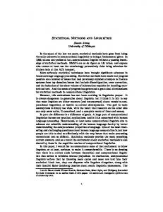
In this talk, our goal is to provide a review on the most used statistical methods to detect and attribute climate changes. The usual statistical framework for detection and attribution in climatology consists of a class of linear regression methods referred to as optimal fingerprinting. Three features of this regression problem are the high dimension (in space and time) with non-sparse covariance matrices, the uniqueness of the observational vector (there is only one Earth) and the limited number of numerical climate runs tainted by model error. These constrains lead to open questions concerning the choice of workable hypothesis and their associated inference schemes. This talk would have a special emphasis on the analysis of extreme events.
About Philippe Naveau After obtaining his PhD in Statistics at Colorado State University in 1998, Dr. Philippe Naveau was a visiting Scientist at National Center for Atmospheric Research in Boulder, Colorado for three years. Then, he was an assistant professor in the Applied Math Dept of Colorado University (2002-2004). Since 2004, he is a research scientist at the French National Research Center (CNRS) and his research work has focused on environmental statistics, especially in analyzing extremes events.
SUMMER SCHOOL #OBIDAM14 / 8-9 Sep 2014 Brest (France) oceandatamining.sciencesconf.org
Overview of statistical methods for detecting and attributing climate changes
´ Alexis Hannart (CNRS) & Aurelien Ribes (Meteo-France) & Philippe Naveau
[email protected] Laboratoire des Sciences du Climat et l’Environnement (LSCE) Gif-sur-Yvette, France
ANR-McSim, ExtremeScope, LEFE-MULTI-RISK
Statistics and Earth sciences
“There is, today, always a risk that specialists in two subjects, using languages full of words that are unintelligible without study, will grow up not only, without knowledge of each other’s work, but also will ignore the problems which require mutual assistance”.
QUIZ (A) Gilbert Walker (B) Ed Lorenz (C) Guillaume Maze (D) Rol Madden
STATISTICS
Detection & Attribution
CLIMATE
Spatial and temporal scales in weather and climate
“Darkness” by Lord Byron
“The bright sun was extinguish’d and the stars did wander darkling in the eternal space, rayless, and pathless, and the icy earth swung blind and blackening in the moonless air ; Morn came and went and came, and brought no day ...” Written in 1816 on the shores of Lake Geneva in the midst of the year without a summer.
Tambora 1815 (illustrations by G. & W.R. Harlin)
) Plutarch noticed that the eruption of Etna in 44 B.C. attenuated the sunlight and caused crops to shrivel up in ancient Rome.
) Benjamin Franklin suggested that the Laki eruption in Iceland in 1783 was related to the abnormally cold winter of 1783-1784.
Natural Climate Variability
Two important natural external forcing factors : Solar irradiance variations (long-trend) Explosive volcanism : Cooling effect on climate (short-lived)
et al. (2001)
1000 –1993
Surface temperature: April–September
Solar forcings dated to 1997.
-3 Hoyt and Schatten (1993) -2
1368 -1
Lean et al. (1995) 1366 1364 1362
0 Beer et al. (1994) 1
[104 atoms / gram ice]
Solar Irradiance [W/m2]
1370
10Be
1372
1360 1358 1600
2 1700
1800
1900
2000
Year A.D. Solar variability (1600-present). The production rate (y-axis) for
10 Be
is reversed since it is inversely correlated wit
Antropogenic forcings
Turner, The Fighting Temeraire - tugged to her Last Berth to be broken up : 1838-39
Detection & Attribution
Detection Demonstrating that climate or a system affected by climate has changed in some defined statistical sense 1 without providing a reason for that change. IPCC Good Practice Guidance Paper on Detection and Attribution, 2010
1. statistically usually, significant beyond what can be explained by variability alone
internal (natural)
Examples of a “Detection” statement
“Warming of the climate system is unequivocal, and since the 1950s, many of the observed changes are unprecedented over decades to millennia. The atmosphere and ocean have warmed, the amounts of snow and ice have diminished, sea level has risen, and the concentrations of greenhouse gases have increased.” IPCC-WG1-AR5 SPM
Observed globally averaged combined land and ocean surface temperature anomaly 1850–2012
(a) 0.6
Annual average
Temperature anomaly (°C) relative to 1961–1990
0.4 0.2 0.0 −0.2 −0.4 −0.6 0.6
Decadal average
0.4 0.2 0.0 −0.2 −0.4
IPCC WG1 AR5 Fig SPM-1a
−0.6 1850
1900
Year
1950
2000
b)
Observed change in surface temperature 1901–2012
IPCC WG1 AR5 Fig SPM-1b
−0.6 −0.4 −0.2
0
0.2
0.4
0.6
0.8
1.0
1.25
1.5
1.75
2.5
(°C)
IPCC-WG1-AR5 SPM ) Observed global mean combined land and ocean surface temperature anomalies, from 1850 to 2012 from th
Examples of a “Detection” statement
These figures and statements don’t say anything about the causes of the observed warming.
Detection & Attribution
Attribution Evaluating the relative contributions of multiple causal factors 2 to a change or event with an assignment of statistical confidence.
2. casual factors usually refer to external influences, which may be anthropogenic (GHGs, aerosols, ozone precursors, land use) and/or natural (volcanic eruptions, solar cycle modulations
Detection & Attribution
Attribution Evaluating the relative contributions of multiple causal factors 2 to a change or event with an assignment of statistical confidence. Consequences Need to assess wether the observed changes are consistent with the expected responses to external forcings inconsistent with alternative explanations
2. casual factors usually refer to external influences, which may be anthropogenic (GHGs, aerosols, ozone precursors, land use) and/or natural (volcanic eruptions, solar cycle modulations
What do you need in D&A ?
Observations of climate indicators Inhomogeneity in space and time (& reconstructions via proxies) An estimate of external forcing How external drivers of climate change have evolved before and during the period under investigation – e.g., GHG and solar radiation A quantitative physically-based understanding How external forcing might affect these climate indicators. – normally encapsulated in a physically-based model An estimate of climate internal variability ⌃ Frequently derived from a physically-based model
Classical assumptions
Key forcings have been identified Signals are additive Noise is additive The large-scale patterns of response are correctly simulated by climate models Statistical inference schemes are efficient
Examples of a “Attribution” statement (see F. Zwiers’ talk)
Attribution results
Others
Data Assimilation
Linear Regression
Inversion Procedure Complexity
Big data : statistical versus numerical models
Climate Model Complexity Toy Models
Alexis Hannart ANR-DADA
Intermediate Complexity Models
GCMs
Data Assimilation for Detection and Attribution
Others
Data Assimilation
Linear Regression
Inversion Procedure Complexity
Big data : statistical versus numerical models
Computational Constraint
Climate Model Complexity Toy Models
Intermediate Complexity Models
GCMs
Two classical statistical approaches in D&A
1- Linear regressions Non-optimal techniques Ordinary and total least square regression Error-in-Variables
Two classical statistical approaches in D&A
1- Linear regressions Non-optimal techniques Ordinary and total least square regression Error-in-Variables 2- FAR (Fraction of Attributable Risk) The FAR = the relative ratio of two probabilities, p0 the probability of exceeding a threshold in a “world that might have been (no antropogenic forcings)” and p1 the probability of exceeding the same threshold in a “world that it is” p1 p0 FAR = . p1 Example of an specific event, the 2003 summer heat wave over Europe.
1- Linear regressions
Outline A quick overview Statistical issues Current solutions
One huge problem (from a stat perspective)
There is only one Earth ! One unique observation, ie. a very long vector (space ⇤ time)
One huge problem (from a stat perspective)
There is only one Earth ! One unique observation, ie. a very long vector (space ⇤ time)
Methods based on learning from a large training set can’t be easily applied
One key idea : use climate models to generate Earth’s avatars !"#$%&'()*#+
,--+.)%/0*1+
!"#$%&'()*#+ 2)-'%+3+&)-/'*0/+
!"#$%& Source : Claudia Tebaldi
The basic regression scheme %&!$'()*+,-$./($01$'+-)$2.-(-$3./0.1)-$+4$501(./$/(6/(--0+1$7)-$ !"#$
Y
! ! X = ( xant , xnat )
Y = X" + # Gabi Hegerl’s presentation at Geneva IPCC WG1/WG2 Meeting in Sept 2009 !"#$%&'()*&+,-#&.%/%("01&2(%1%34,5)3&,4&+%3%6,&7899&:+;%%53/&)3&?@AB&!%24%*-%(&=CCD&
The basic Gaussian regression scheme
“ ˆ = XT⌃
1
X
”
1
XT⌃
1
with under the Gaussian assumption with know ⌃ “ E( ˆ) = and Var ( ˆ) = X T ⌃
Y
1
X
”
1
The basic Gaussian regression scheme
“ ˆ = XT⌃
1
X
”
1
XT⌃
1
with under the Gaussian assumption with know ⌃ “ E( ˆ) = and Var ( ˆ) = X T ⌃ Practical questions = 0 + CI ? = 1 +CI ?
Y
1
X
”
1
An example
Joint 90% confidence region for ANT 1 Oand 2013 M I Nand E T A LTXx . NAT detection in TNn CTOBER
Min et al, 2013, Fig. 9
FIG. 9. The joint 90% uncertainty range for the ANT and NAT scaling factors when temperature extre ANT (x axis) and NAT signals (y axis) global-mean extremes (TNn, TXn, and TN Details: 1951-2000 TNn and TXxsimultaneously: from HadEX (top) (Alexander et al,cold 2006), decadal extremes (TNx, TXx, and TNx 1 TXx). The error CMIP3 bars indicate one-dimensional 5%–95% time averaging, “global” spatial averaging, models (ANT – 8 models, 27ranges of the s The dashed lines represent and unity.158 chunks) runs; ALL horizontal/vertical – 8 models, 26 runs; control –zero 10 models, Source : Francis Zwiers
5-yr means. Figure 7 shows two-signal analysis results
detection results for global- a
An example
Calculating attributed change
Usual approach is to calculate trend in signal, !"#$%&'($)*&+,&-.#/&01234& 56$7*/(&21& 8955&:;8&!")*6&/#*&? multiply by scaling factor, and apply scaling factor & uncertainty Observed warming trend and 5-95% uncertainty range based on HadCRUT4 (black). Attributed warming trends with assessed likely ranges (colours).
IPCC WG1 AR5, Fig 10.5
Figure Source : Francis Zwiers
10.5:&"EA7@"#*=&+H$(=4&)@(&$**("H.*$H%/&F$(>"#C&*(/#E=&@I/(&*6/ 2JK2L0121&7/("@E&E./&*@&F/%%A>"M/E&C(//#6@.=/&C$=/=&+;N;4O&@*6/(&$#*6(@7@C/#"P&)@("#C=&+Q$'/C%'>$ D;#05/4%0;%$'%B%'$EF*GH$"2&"$276&0$/05'7%0;%$2&.$&"$'%&."$4#7='%4$ "2%$3/.C$#5$&$2%&"9&B%$%:;%%4/01$"2/.$"23%.2#'4$6&10/"74%I
!"#""$%"$&'($)**+
Revisiting the-2003 European heatwave with counterfactual theory vent attribution illustration on 2003 European heatwave !
Step 2: EVT extrapolation (GEV) based on HIST and NAT ensembles (Hadley center model) => two distributions of Z.
EVT extrapolation (GEV) based on HIST and NAT ensembles (Hadley center model)
p0 = 0.0008 (1/1250), p1 = 0.008 (1/125)
Event attribution - illustration on 2003 European heatwave !
Step 3: p0 = 0.0008 (1/1250), p1 = 0.008 (1/125)
PN = 0.9, PS = 0.0072, PNS = 0.0072 « CO2 emissions are very likely to be a necessary cause, but are virtually certainly not a sufficient cause, of the 2003 heatwave. » This highlights a distinctive feature of unusual events: several necessary causes may often be evidenced but rarely a sufficient one
« It is very likely (>90%) that CO2 emissions have increased the frequency of occurrence of 2003-like heatwaves by a factor at least two »
=
« CO2 emissions are very likely to be a necessary cause of the 2003 heatwave. »
Event attribution - summary !
«!Have CO2 emissions caused the 2003 European heatwave?!»
!
The answer is greatly affected by: — — —
how one defines the event «!2003 European heatwave!», what is the temporal focus of the question, whether causality is understood in a necessary or sufficient sense.
Precise causal answers about climate events critically require precise causal questions.
Event attribution - necessary and sufficient causation !
Which matters for event attribution: PN, PS or PNS ?
!
The ex post perspective (judge) : — — —
!
The ex ante perspective (policy maker) — —
!
«who is to blame for the weather event that occurred ?» insurance, compensation, loss and damage mechanisms (e.g. Warsaw 2013) PN matters, not PS.
«what should be done today w.r.t. events that may occur in the future?» PS matters for assessing the cost of inaction, PN for assessing the benefit of action.
The dissemination perspective (media, IPCC) — —
PNS is a trade off between PN and PS. good candidate for a single metric as it avoids explaining the distinction.
PN, PS and PNS all matter
Summary EIV
FAR
Causality
STATISTICS
Linear regression
Internal variability
Detection & Attribution
Ensemble runs
Forcings
CLIMATE
Control runs
Observations
Statistical challenges
Making links with other communities (machine learning, data mining, ...) Reframing FAR D&A questions and definitions by injecting error models Investigating further regression models within the counterfactual theory Finding ways to estimate non-sparse and big covariance matrices Moving away from the Gaussian framework for extremes Uncertainty of FAR as the ratio of two small probabilities Adding more physics within the statistical model (data assimilation) Taking advantage of fast algorithms Add a Bayesian flavor to clarify assumptions Improve climate models and their use (design experiments)
A very short bibliography Allen, M.R., and S.F.B. Tett, 1999 : Checking for model consistency in optimal fingerprinting. Clim. Dyn., 15, 419–434. 3. Allen, M.R., and P.A. Stott, 2003 : Estimating signal amplitudes in optimal fingerprinting, Part I : Theory. Clim. Dyn., 21, 477–491. Hannart, A., A. Ribes, and P. Naveau, 2014 : Optimal fingerprinting under multiple sources of uncertainty, Geophys. Res. Lett., 41, 1261–1268. Hannart, A. and P. Naveau, 2014. Estimating high dimensional covariance matrices : A new look at the Gaussian conjugate framework J. Multi. Analysis. Hannart, A., Pearl J. Otto F., P. Naveau and M. Ghil. (submitted). Counterfactual causality theory for the attribution of weather and climate-related events Huntingford,C.,P.A.Stott,M.R.Allen,andF.H.Lambert,2006 :Incorporating model uncertainty into attribution of observed temperature change. Geophys. Res. Lett., 33. Ledoit O,Wolf M(2004),A well-conditioned estimator for large dimensional covariance matrices. J. Multivar. Analysis. ,88 :365-411 J. Pearl (2000), Causality : models, reasoning and inference, Cambridge University Press. Ribes A, Planton S, Terray L,2013a : Application of regularized optimal fingerprinting to attribution. Clim Dyn, doi :10.1007/s00382-013-1735-7 Hegerl, G. C., et al., 2010 : Good practice guidance paper on detection and attribution related to anthropogenic climate change. IPCC WG1. IPCC, 2013, The physical science basis. WG1 Zhang,X.,H. Wan,F.W. Zwiers, G.C. Hegerl, and S.-K.Min,2013 :Attributing intensification of precipitation extremes to human influence, Geophys. Res. Lett., 40, 5252–5257, doi :10.1002/grl.51010.
Statistics and Earth sciences
and named the “Southern Oscillation” (Walker, 1924). At that time, the approach most prevalent in the statistical analysis of weather variables was to search for deterministic cycles through reliance on harmonic analysis. Such cycles included those putatively as-
“There is, today, always a risk that specialists in two subjects, using languages full of words that are unintelligible without study, will grow up not only, without knowledge of each other’s work, but also will ignore the problems which require mutual assistance”. QUIZ (A) Gilbert Walker
F IG . 3. Photograph of Sir Gilbert T. Walker (source: Royal Society; Taylor, 1962).
Necessary and sufficient causation
Overview of the theory - necessary and sufficient causation !
The judge perspective: — — — — —
!
defendant A shot a gun at random in a seemingly desert place. B stood one kilometer away and was unluckily hit right in between the eyes. PN ~ 1, PS ~ 0. but A is an obvious culprit for the death of B from a legal perspective. only PN matters here, PS does not.
The policy-maker perspective: —
what is the best policy to achieve a given objective ? (say, reducing accidental gunshot mortality) ! ! !
—
prohibiting guns sales => PN = .., PS ~ 1 restricting guns sales => PN = .., PS = … better informing gun owners on safety => PN = .., PS = …
both PN and PS matter to assess efficiency.