Mathware & Soft Computing 12 (2005), 97-106
p-Median Problems in a Fuzzy Environment D. Kutangila-Mayoya, J.L. Verdegay Dept. of Computer Science and Artificial Intelligence University of Granada 18071 Granada (Spain)
[email protected],
[email protected]
Abstract
In this paper a formulation for the fuzzy p-median model in a fuzzy environment is presented. The model allows to find optimal locations of p facilities and their related cost when data related to the node demands and the edge distances are imprecise and uncertain and also to know the degree of certainty of the solution. For the sake of illustration, the proposed model is applied in a reduced map of Kinshasa (Democratic Republic of Congo) obtaining results which are rather than realistic ones
Keywords: Fuzzy graphs, public transport, location problems .
1 Introduction Democratic Republic of Congo (formerly Zaire) has a total superficie of 2.344.000 sq km., more than 45.000.000 inhabitants and it is situated in central Africa. It borders on Angola in the southwest and west, on Cabinda and the Republic of the Congo in the west, on the Central African Republic and Sudan in the north, on Uganda, Rwanda, Burundi, and Tanzania in the east, and on Zambia in the southeast. The country is divided into ten provinces (Bandundu, Bas-Congo, Équateur, Kasai-Occidental, KasaiOriental, Katanga, Maniema, Nord-Kivu, Orientale, and Sud-Kivu) and a federal district (which includes Kinshasa). In addition to Kinshasa, other major urban areas include Boma, Bukavu, Kalemie, Kamina, Kananga, Kisangani, Kolwezi, Likasi, Lubumbashi, Matadi, Mbandaka, and Mbuji-Mayi. Kinshasa is its capital and largest city. The town of Kinshasa, political capital of the Democratic Republic of Congo, undergoes a multiform crisis. No sector is saved, including those which are used for the development of the others, in particular the public transport. However, one can speak 97
98
D. Kutangila & J.L. Verdegay
about no development by excluding that of the public transport, this last being an irreplaceable accompaniment of the economic development. Several causes are at the basis of this crisis: 1. The configuration of the town: Kinshasa is designed in such a way that in the north, there is a major concentration of all the useful activities, and in the south dormitory town where people live. At the independence, this configuration was not modified, and it is this configuration which justifies the pendular motions in Kinshasa. 2. The demographic growth: In 1960, Kinshasa counted 400.000 inhabitants, but in 2001, the population of the town was of more than 6.000.000 inhabitants. Kinshasa will thus be counted among the largest cities of the world, because of its population. According to statistical projections, in 2015 Lagos will reach 24 million inhabitants [8], Cairo more than 16,5 million inhabitants [9] and Kinshasa 10 million inhabitants. In 2015 among the 15 largest cities in Africa, it is necessary to count Cairo, Lagos and Kinshasa. The other cities will be Asian. 3. The spreading out of the city: Demographic growth involves the spreading out of the city (approximately 10.000 km2) what definitely lengthens the distances. 4. A null and void and degraded roadway system: On the 5.109 km of roads, 548 km only are covered (asphalted). Therefore 4561 km of roads are out of ground. Kinshasa counts only 5 primary roads: the avenues of the IPN, 24 Novembre, Kasavubu, University, ant Boulevard Lumumba, from where traffic congestion, and 5. A transport offer lower than the request: The studies show that there are 3.600.000 of displacements per day in the town of Kinshasa, but only 196.100 displacements are done by means of transport. Therefore 5,44% of request satisfied and 94,55% of no satisfied request. The 5,44% of displacements are transported by 1.142 cars. Search shows that on 196.100 displacements, 3% use the car private, 40% use the bus or the train, 20% use the taxi and 36 % move by walking. As it is patent the problem of the public transport is a growing thorny problem for the people of Kinshasa which deserves a great deal of effort for solution. From a theoretical point of view, as soon as a city reaches 1.000.000 inhabitants, it is automatically necessary to change the system of transport, i.e., to give up the buses. Indeed, the capacity of a bus is very low (80 people). However since 1970 the regional govern is trying to change the system of transport in Kinshasa in a number of ways: 1. By adopting new means of transport of mass, i.e., the Subway, the tram or the train. The subway: The construction of the underground subways is a too heavy and expensive investment. The ground of Kinshasa is not favourable with the construction of the underground subways because of the internal sea (the ground of Kinshasa rests on water). The tram shares the road with the vehicles. With five too small roads, that is impossible. The train: Since the rail network already exists and the rails serve the four corners of the city, one of the tracks of solution is the rehabilitation of the train and the electrification of the rail network 2. By rehabilitation and town-planning: The city grows but there are no roads. There are no East-West roads (transverse roads) because of the mountains. From where it
p-Median Problems in a Fuzzy Environment
99
is necessary to create transverse roads and to asphalt the roads of service roads like Mokali, Ndjoku, etc 3. By promoting the river public transport by setting up of the boat-buses along the Congo river until Maluku. 4. By the scattering of the great activities of the town of Kinshasa while establishing of the shopping centres through the city. 5. By the optimization of the transport networks (terrestrial, railway and river). The attempt here would be to get alternative transportation networks in Kinshasa according to the four first tracks of solution, and 6. By proposing and designing new networks of transport based on the solution of tailored locations problems which say us, for instance where to locate bus stops, underground or tram stations, etc. A Location Problem deals with the choice of a set of points for establishing certain facilities in such a way that, taking into account different criteria and verifying a given set of constraints, they optimally fulfil the needs of the users. Some of the main location problems are modelled on a network or a graph. Thus, the vertices of the network represent the points where the users that demand the facility are, and the edges reveal the existence of a certain link between the vertices (for instance, roads joining cities). In general, the graphs represent deterministic situations where the points of demand and the links joining them are known. Originally proposed by Hakimi (1964, 1965) who demonstrated the possibility of locating optimally at least p facilities on the network nodes, the crisp p-median problem consists of selecting p facility nodes or locating p facilities on finite, connex, simple, no directed, determinist and static graph such that the weighted total distance between all the demand nodes and their closest facility nodes is minimized. This problem has been investigated by several authors [14, 7, 1, 10, 2, 3, 4, 5, 13, 8, 12, 15, 9, 16 and recently 11). Generally, the crisp p-median problem is mathematically formulated as follows:
z* = min ∑∑wd i ij xij i
s.t.
(1)
j
∑x
ij
=1,
∀i ∈N
(2)
∀i, j ∈N,
(3)
j
xij ≤ y j ,
∑y = p,
(4)
j
j
xij , yj ∈{0,1}
∀i, j ∈N,
where i is the demand node, j is the facility node,
(5)
wi is the demand at node i, d ij is the
distance of the shortest path between nodes i and j, xij is 1 if the node i is assigned to
100
D. Kutangila & J.L. Verdegay
facility j and 0 otherwise, y j is 1 if there is a facility at node j and 0 otherwise, and p is the number of facilities to be located. The objective function (1) minimizes the total weighted distance between all the demand nodes and their closest facility nodes. The set of restrictions (2) formalizes the single assignment of demand nodes to facility nodes. The set of restriction (3) prohibits assignment to node that has not facility. (4) fixes the number of facilities to be located to p and (5) formalizes the binary nature of assignment-localization decision. The crisp p-median problem is applicable in the deterministic environment where all the data are certain. However the real world is full of uncertainty, and we often are given imprecise and uncertain data. In this case, we need to know how certain is our results (the degree of certainty of our results). We refer to this problem as the fuzzy p-median problem. Consequently, the aim of this paper is to present a new model of fuzzy pmedian problem, what is addressed in the following section, and then to propose a solution method that, finally is illustrated by means of a real problem which is tailored to to the objectives of a scientific paper like this.
2 A model of the fuzzy p-median problem Let us consider a network G = (N,A), where N = {1,…,n} is the set of nodes and A is a set of existing edges between each nodes pair (i,j) in the graph. Each node i∈N has a positive weight wi representing the population (demand) at the node. Each edge (i,j) also has a positive weight lij that represents the length of the edge. With the weight of the existing edges, we calculate a matrix D of distances dij of the shortest paths between the nodes (i,j), ∀ i,j ∈ N, i ≠ j. Under a uncertainty environment, the values wi and lij are vague ones. With such data, it is obvious that optimal locations and the cost obtained using the crisp p-median model are not certain. Thus, the basic problem is to determine the degree of certainty of the optimal locations and their related cost when the values wi and lij are uncertain. Therefore, we define the following fuzzy subsets, for the fuzzy p-median problem: • W = {( wi|µW(wi))}, ∀ i ∈ N, is the fuzzy subset of the most certain weights wi. µW(wi) is the degree of belongingness of the node i to the fuzzy subset W, in other words µW(wi) is the degree of certainty of the weight wi. • L = {( lij|µL(lij))}, ∀ i,j ∈ N, is the fuzzy subset of the most certain lengths lij of the edges between the nodes i and j. µL(lij) is the degree of belongingness of the length lij to the fuzzy subset L, in other words µL(lij) is the degree of certainty of the length lij. • Using the subset L, we will build a fuzzy matrix D of the most certain distances dij of the shortest paths between the nodes pairs (i,j). We define the fuzzy matrix by D = {( dij|µD(dij))}, ∀ i,j ∈ N where dij is the distance of the shortest path between nodes i and j calculated using Floyd-Warshall Algorithm [6] and µD(dij) is the degree of certainty of dij.
p-Median Problems in a Fuzzy Environment
101
The goal of both fuzzy and crisp p-median problem is to find optimal locations of p facilities such that the total weighted distance or the total cost of travel from each demand node to its closest facility node is minimized. The fuzzy p-median particular aspect is to determine the degree of certainty of the optimal locations and cost. Thus, the difference between the crisp p-median problem and the fuzzy one is: • The crisp p-median problem handles precise and certain data with degree of certainty 1 and consists of finding optimal locations of p facilities with their related cost having a degree of certainty 1. • The fuzzy p-median problem handles imprecise and uncertain data with degree of certainty between 0 and 1 and consists of finding optimal locations for p facilities with their related cost having degree of certainty mapped in the unit interval [0,1]. Therefore we can conclude that the fuzzy p-median problem is a generalization of the crisp one and is more realistic than the crisp problem since the real world is full of uncertainty, and consequently we can formulate the fuzzy p-median model as it follows: ( z*|λ*) = min ∑i ∑j(wi|µW(wi))( ( dij|µD(dij))xij
(1)
∑j xij = 1,
∀i∈N
(2)
∀ i,j ∈ N
(3)
s.t.
xij ≤ yj, ∑j yj = p, xij, yj ∈ {0,1},
(4) ∀ i,j ∈ N
(5)
where z* = optimal transport total cost, λ* = degree of certainty of the optimal cost (optimal solution) W = fuzzy subset of the most certain weights wi of the nodes i. D = fuzzy matrix of the most certain distances dij of the shortest paths between all the nodes pairs (i,j). i ∈ N = demand nodes, j ∈ N = facility nodes, wi = uncertain population or demand of the nodes i, µW(wi) = degree of certainty of wi. dij = uncertain distance of the shortest path between the nodes i and j, µD(dij) = degree of certainty of dij. dij = 1 if the node i is assigned to the node j and 0 otherwise, yj = 1 if there is a facility at j and 0 otherwise, p = number of facilities to be located. The fuzzy p-median model we have formulated must be applied on fuzzy graphs. In these graphs, no having exact demands at each node nor exact distances among edges, we express these quantities or values following them with their degrees of certainty. Consequently, the objective function of the fuzzy p-median model for such a graph doesn’t calculate only the optimal cost but also its degree of certainty.
102
D. Kutangila & J.L. Verdegay
3 A Solution approach In the objective function of the model we use the aggregation operator ∑ for the sum. This operator will be used to calculate the optimal cost. With regard to what operation we must effectuate on the degrees of certainty in order to obtain the degree of certainty of the final solution we consider the following. It is well-known that elements of a collection of fuzzy sets can be combined to produce a single fuzzy set through aggregation operations [18]. This is the case, for instance, in the intersection and union of any number of fuzzy sets. In general, many other types of aggregation may be performed on fuzzy sets. Here we will focus on aggregations A:[0,1]→[0,1] satisfying the following requierements: • Boundary conditions: A(0,…,0) = 0 and A(1,…,1) = 1 • Monotonicity: A(x1,…,xn) ≥ A(y1,…,yn) if xi ≥ yi, i = 1,...,n The aggregation operators discussed in [18] are the compensatory operators defined by Zimmermann and Zysno (1980), the symmetric sums by Dubois and Prade (1980), the averaging operators by Dyckhoff and Pedrycz (1984) and the ordered weighted averaging operator (OWA) by Yager (1988). In our model we are going to use averaging operators. An averaging operator (generalized mean) for n arguments is idempotent and commutative, in addition to fulfilling monotonicity and boundary conditions. As discussed in Dyckhoff and Pedrycz (1984), the generalized mean takes the form
A ( x1 ,..., xn ) =
p
1 n p ( xi ) , p ∈ R, p ≠ 0. ∑ n i =1
It is important to note that the family of generalized means subsumes some wellknown cases of fuzzy-set operators. In particular, we obtain 1. Arithmetic Mean (p = 0)
A ( x1 ,..., xn ) =
1 n ∑ ( xi ) . n i =1
2. Geometric Mean (p → 0)
A ( x1 ,..., xn ) = ( x1 ,..., xn ) n 1
3. Harmonic Mean (p = -1)
A ( x1 ,..., xn ) =
n n
i =1
4. Minimum (p → -∞) 5. Maximum (p → ∞)
1
∑x
i
A ( x1 ,..., xn ) = min ( x1 ,..., xn ) A ( x1 ,..., xn ) = max ( x1 ,..., xn ) .
The parameter p can be referred to as a compensation factor.
p-Median Problems in a Fuzzy Environment
103
In our model of the fuzzy p-median problem, the degrees of certainty are going to be handled using the arithmetic mean operation instead of the sum operation and the minimum operation instead of the multiplication operation. That is, the model that we have presented is going to be solved in two steps: first, the crisp p-median is normally calculated with approximative data in order to find the crisp optimal locations and cost, i.e. the above model is used without the degrees of certainty, like this: z* = min ∑i ∑jwi dijxij s.t. ∑j xij = 1, xij ≤ yj, ∑j yj = p, xij, yj ∈ {0,1}
(1) ∀i∈N ∀ i,j ∈ N ∀ i,j ∈ N
(2) (3) (4) (5)
Second, the degrees of certainty are used in the following submodel in order to calculate the degree of certainty of the crisp solution obtained in step 1:
1 n−p 1 p λ = ∑min µW ( wi ) , µD ( dij ) xij ∑ n − p i=1 p j=1 *
(
)
s.t. ∑j xij = 1, ∀ i = 1,…,n - p µW(wi), µD(dij) ∈ [0,1] ∀ i = 1,…,n – p, j = 1,…, p If wi and dij are certain, i.e. if µW(wi) = 1, ∀ i ∈ N and µD(dij) = 1, ∀ dij ∈ D, then λ* = 1 and there is no need of going to step 2, since this is a crisp p-median. But if wi and dij are uncertain, i.e. if µW(wi) ∈ [0,1], ∀ i ∈ N and µD(dij) ∈ [0,1], ∀ dij ∈ D, then, by the step 2, we have λ* ∈ 1; this is a fuzzy p-median. Thus, the fuzzy p-median is a generalization of the crisp one.
4 Illustrative example The map of Kinshasa can be seen in Figure 1. This is a map that because of several reasons, far from the aim of this paper, can be considered as fuzzy, and hence also the nodes, distance, demands, etc. As the real situation is very complex, here for the sake of illustration in order to find two optimal locations of bus station, we will consider only a fuzzy graph of western Kinshasa, with uncertain demands and distances as follow. First seven nodes (Binza IPN, Binza Delvaux, Binza Ozone, Binza Pompage, Kintambo Magasin, Parking Bandal and Selembao Marché), will be considered. Second, the distances between nodes (Table 2) are approximate ones. In this way, all of them will be considered as fuzzy ones with degrees of membership equal in all the case to 0.75. Take
104
D. Kutangila & J.L. Verdegay
into acccount that our main aim here is only to show how the proposed model solve a problem which although real, here is simplified. Node 1 2 3 4 5 6 7
1 2 3 4 5 6 7
Designation
Demand
Binza IPN 26.13 Binza Delvaux 26.13 Binza Ozone 26.13 Binza Pompage 26.13 Kintambo Magasin 14.80 Parking Bandal 30.58 Selembao Marché 44.97 Table 1: Nodes in the network 1 0,00 3,00 7,00 11,20 8,00 7,60 3,60
2 3,00 0,00 4,00 8,20 5,00 9,50 6,60
3 4 5 7,00 11,20 8,00 4,00 8,20 5,00 0,00 6,40 3,20 6,40 0,00 3,20 3,20 3,20 0,00 7,70 7,70 4,50 10,60 11,70 8,50 Table2: Distances between nodes
Degree of certainty 0.75 0.70 0.80 0.65 0.70 0.70 0.65
6 7,60 9,50 7,70 7,70 4,50 0,00 4,00
7 3,60 6,60 10,60 11,70 8,50 4,00 0,00
Then it is easily obtained that the optimal locations are nodes 5 and 7 with the cost of 514,270, and the degree of certainty of these locations and their related cost is 0,69.
Conclusion We have seen that the crisp p-median problem is applied on deterministic graphs to locate p facility centres such that the weighted sum of the distances between all the demand nodes and their closest facility centres is minimized. The resulted solution is certain and has the degree of certainty equals to 1. We have formulated the model of the fuzzy p-median problem applicable to fuzzy graphs where data are uncertain. That model has allowed us to know the degree of certainty of the uncertain solution obtained on uncertain data.
Acknowledgement Research supported under project TIC2002-04242-CO3-02. The first author is a grantholder of the Spanish Foreign Relations Minister
p-Median Problems in a Fuzzy Environment
105
Figure 1: Map of Kinshasa town
References [1] Bowerman, R.L., P.H. Calamai, G.B. Hall, The demand partitioning method for reducing aggregation errors in p-median problems, Computers & Operations Research 26 (1999) 1097 – 1111 [2] Canós, M.J., C. Ivorra, V. Liern, An exact algorithm for the fuzzy p-median problem, European Journal of Operational Research 116 (1999) 80 – 86 [3] Canós, M.J., C. Ivorra, V. Liern, Finding satisfactory near-optimal solutions in location problems, J.L. Verdegay Editor, Fuzzy Sets Based Heuristics for Optimization, 126 (2002) 265 – 276 [4] Canós, M.J., C. Ivorra, V. Liern, The fuzzy p-median problem: A global analysis of the solutions, European Journal of Operational Research 130 (2001) 430 – 436 [5] Canós, M.J., C. Ivorra, V. Liern, Un algoritmo de intercambio para el problema borroso de la p-mediana cuando el coste óptimo es desconocido, Emergent Solutions for Information and Knowledge Economy, Proceedings of the 10th SIGEF Congress 2 (October 2003) 79 – 89
106
D. Kutangila & J.L. Verdegay
[6] Cormen, T.H., C.E. Leiserson, R.L. Rivest, Introduction to Algorithm, The MIT Press (1989), 1026 [7] Erkut, E., B. Bozkaya, Analysis of aggregation errors for the p-median problem, Computers & Operations Research 26 (1999) 1075 – 1096 [8] García-López, F., B. Melián-Batista, J.A. Moreno-Pérez, J.M. Moreno-Vega, Parallelization of scatter search for the p-median problem, Parallel Computing 29 (2003) 575 – 589 [9] Hansen, P., N. Mladenovíc, Variable neighbourhood search for the p-median, Location Science 5 (1997) 207 – 226 [10] Hribar, M., M.S. Daskin, A dynamic programming heuristic for the p-median problem, European Journal of Operational Research 101 (2001) 430 – 436 [11] Kutangila, D., J.L. Verdegay, Fuzzy graphs as basis for solving some public transportation problems in Kinshasa, Emergent Solutions for Information and Knowledge Economy, Proceedings of the 10th SIGEF Congress 2 (October 2003) 71–77. [12] Lorena, L.A.N., E.L.F. Senne, A column generation approach to capacitated pmedian problems, Computers & Operations Research 31 (2004) 863 – 876 [13] Rolland, E., D.A. Schilling, J.R. Current, An efficient tabu search procedure for the p-median problem, European Journal of Operational Research 96 (1996) 329 – 342 [14] Rosing, K.E., C.S. ReVelle, D.A. Schilling, A gamma heuristic for the p-median problem, European Journal of Operational Research 117 (1999) 522 – 532 [15] Serra, D., V. Marianov, The p-median problem in a changing network: the case of Barcelona, Location Science 6 (1998) 383 – 394 [16] Zhao, P., R. Batta, Analysis of centroid aggregation for the Euclidian distance pmedian problem, European Journal of Operational Research 113 (1999) 147 – 168 [17] Kauffman, A., Introduction à la théorie des sous-ensembles flous, Masson et Cie, Vol. I (1973) [18] Pedrycz, W., F. Gomide, An introduction to fuzzy sets : Analysis and design, The MIT Press, London,.